Predicting MPEG Execution Times - CiteSeerX

Predicting MPEG Execution Times Andy Bavier and Brady Montz and Larry L. Peterson TR 97-15

Abstract This paper reports on a set of experiments that measure the amount of CPU processing needed to decode MPEG-compressed video in software. These experiments were designed to discover indicators that could be used to predict how many cycles are required to decode a given frame. Such predictors can be used to do more accurate CPU scheduling. We found that by considering both frame type and size, it is possible to construct a linear model of MPEG decoding with R2 values of 0.97 and higher. Moreover, this model can be used to predict decoding times at both the frame and packet level that are almost always accurate to within 25% of the actual decode times. This is a surprising result given the large variability in MPEG decoding times, and suggests that it is feasible to design systems that make quality of service guarantees for MPEG-encoded video, rather than less variable encodings, such as JPEG.

Department of Computer Science The University of Arizona Tucson, AZ 85721

1 Introduction The ability of modern processors to decode MPEG compressed video in realtime has led to users wanting to run a mix of applications that includes both MPEG video streams and other realtime and non-realtime tasks. The problem that arises in this situation is how to schedule these applications on the CPU, which is in turn complicated by the need to know how much execution time a given realtime task is going to take before the task can be scheduled. The need to have accurate information about the required MPEG execution time exists at two different levels. At a coarse-grained level, knowing the number of cycles (percentage of the CPU) needed to decompress a given video stream, when averaged over a relatively long time interval, is needed to do load control—that is, to determine how many simultaneous video streams can be supported. At a fine-grained level, knowing how long a particular MPEG frame will take to decode can be used by the scheduling algorithm. The latest acceptable start time for the decoding task is the deadline of that frame minus the length of time to decode that frame. Scheduling algorithms are now being designed to exploit such information [1, 7, 2]. This paper focuses on the fine-grain predictors that are suitable for scheduling, but in doing so, also lays the ground work for designing better load control mechanisms. The difficulty is that MPEG decoding does not consume a constant amount of processing, due in part to the fact that a given MPEG video stream contains different frame types, and in part to the potential wide variation between scenes (e.g., talking heads versus action). This makes prediction of the time to decode the next frame based on past behavior difficult. What is needed are finer-grained indicators that can be used to predict future execution times. The current lack of such indicators is one factor limiting systems that make quality of service guarantees to JPEG videos, rather than the more ubiquitous MPEG format. Towards this end, this paper reports on a set of experiments designed to measure the amount of CPU processing needed to decode MPEG compressed video on a modern processor. An analysis of these experiments is presented in Section 3. We then use these results to construct a set of estimators, which are described and evaluated in Section 4. The main results, which are summarized in Section 5, are that it is possible to construct linear models of MPEG decoding with R2 values of 0.97 and higher, and that these models can be used as the foundation for predicting execution time needed at both the packet and frame levels (for the purpose of scheduling) to within 25% of the time actually taken to decode these packets and frames.

2 MPEG Decoding Before presenting our results, we first give a brief overview of MPEG. We also describe the execution environment in which the measurements were taken, and in which the resulting estimators were eventually employed.

2.1 MPEG The MPEG video compression standard defines a video stream as a sequence of still images (frames) that are displayed at some rate, for example, 30 frames per second (fps) [4]. Each frame is of a particular type: I frames (intrapicture), P frames (predicted picture) and B frames (bidirectional predicted picture). I frames are self-contained, complete images. P and B frames are encoded as differences from other reference frames. Only I and P frames may be used as reference frames. A group of pictures (GOP) is a sequence of frames from one I frame to the next; e.g., I B B P B B I. Note that different videos use different GOP sequences. A given frame consists of a collection of macroblocks, each of which corresponds to a 1616 block of pixels. The MPEG algorithm actually operates on macroblocks, not entire frames. In fact, not all the macroblocks contained in a frame of a given type are necessarily encoded in accordance with that type. It is possible, for example, to have an I encoded macroblock as part of what is otherwise a B frame. In way of a brief overview to the computational requirements of MPEG, we observe that I macroblocks are the most expensive to decode, as doing so involves the computationally expensive Discrete Cosine Transform (DCT). Before the DCT can be applied, however, the values are first run-length decoded, Huffman decoded, and passed through a reverse quantization process. In contrast, the processing required to decode B and P macroblocks is less demanding. Consider the decoding of a B macroblock, which depends on both a previous and a subsequent I or P frame. Each B

1

macroblock is represented with a 4-tuple: (1) a coordinate for the macroblock in the frame, (2) a motion vector relative to the previous reference frame, (3) a motion vector relative to the subsequent reference frame, and (4) a delta for each pixel in the macroblock (i.e., how much each pixel has changed relative to the two reference pixels).1 For each pixel in the macroblock, the first task is to find the corresponding reference pixel in the past and future reference frames using the two motion vectors. Then, the delta for the pixel is added to the average of these two reference pixels.

2.2 Scout OS We measured MPEG decoding performance in the context of the Scout operating system [6]. Scout is a configurable OS explicitly designed to support data streams such as MPEG-compressed video. Specifically, Scout defines a path abstraction that encapsulates data as it moves through the system, for example, from input device to output device. In effect, a Scout path is an extension of a network connection through the OS. Each path is an object that encapsulates two important elements: (1) it defines the sequence of code modules that are applied to the data as it moves through the system, and (2) it represents the entity that is scheduled for execution. Display Device

Disk Device

VGA

SCSI

WIMP

UFS

MPEG

FTP

MFLOW TCP UDP IP IP ETH

ETH

Network Device

Network Device

Figure 1: Example Scout Paths Figure 1 schematically depicts a pair of Scout paths: the path on the left implements an MPEG video stream that transforms network packets into video frames, and the path on the right corresponds to an FTP path that moves incoming network packets to a disk device. In this figure, each path has a source and a sink queue, and is labeled with the sequence of software modules that define how the path “transforms” the data it carries. Focusing on the MPEG path, ETH is the device driver for the network card, IP and UDP are the conventional network protocols, MFLOW is an MPEG-aware transport protocol, MPEG implements the decompression algorithm described in Section 2.1, WIMP is the window manager, and VGA is the device driver for the graphics card. Operationally, network packets that arrive for a particular video stream are inserted into the source queue for the corresponding Scout path. Since there may be multiple MPEG paths active in the system at a given time, Scout first classifies each incoming packet according to the path it belongs to; we take a closer look at packet classification in Section 4. Once enqueued on a path, a thread is scheduled to shepherd this message along the path; this thread inherits its scheduling parameters from the path, as described below. When the thread runs, it executes the sequence of modules 1 P macroblocks are decoded in a similar fashion, except they depend on just the previous reference frame, and so include only a single motion vector. Also, a B-block can optionally be encoded with just one motion vector, rather than two.

2

associated with the path, and deposits the message in the sink queue. The display device periodically removes frames from the sink queue and displays them. There are two reasons why predicting the time to decode helps the implementation of a scheduler that provides quality of service guarantees. First, due to video’s realtime constraints, each frame must be decoded by a certain time. It is only by knowning how long this thread will run that we can determine the latest time the thread must start executing. Classical realtime scheduling algorithms, such as Earliest Deadline First (EDF) [3], do not require knowing the execution time, but they have the limitation of not operating well under load. This makes EDF inappropriate when one is trying to mix realtime and non-realtime tasks. Scheduling both realtime and non-realtime tasks under load requires knowing how long a realtime task is going to run [1, 7, 2]. To illustrate how a scheduling decision might be made, suppose the graphics device is draining the sink queue at a rate of 30 messages (frames) per second, and after consuming a frame at time t there are two additional frames on the queue, then the path knows that the deadline for producing the next frame is t + 66ms. That is, the thread responsible for shepherding messages from the source queue to the sink queue must complete by time t + 66ms. If the path also knows that it takes 10ms to generate new frame, then the path assigns the thread a latest acceptable start time of t + 66ms ? 10ms. Estimating the execution time—e.g., 10ms in this example—is the goal of this paper. The second reason stems from Scout’s use of cooperative multithreading. When a thread is scheduled to run along a path, it owns the CPU until it reaches the end of the path or explicitly yields.2 If the scheduler is faced with multiple threads which can run next, it is impossible to predict the effect running one will have on the others’ ability to meet their deadlines without knowing how long that thread will run. There is one additional nuance to video decoding. When the thread finally gets to run, it is allowed to execute the path one or more times, resulting in the consumption of one or more network packets. In fact, executing an MPEG path multiple times may be required to produce a single video frame. This is because there is not a one-to-one relationship between network packets (in the source queue) and video frames (in the sink queue). Quite often a single frame spans multiple network packets, although it is also possible for multiple compressed video frames to fit in a single network packet. In our case, the protocol MFLOW is responsible for fragmenting frames into fixed-sized packets. The important characteristic of this fragmentation algorithm is that each network packet carries an integral number of macroblocks—i.e., a single macroblock is never split across packet boundaries—and packets containing the last macroblock of a frame denote this fact with a special End-Of-Frame (EOF) marker. The path object can be instrumented with multiple cycle counters. For example, by reading the cycle counter when a path starts running and again when it finishes, it is possible to measure the number of cycles required by a single execution of a path; this corresponds to the time required to consume a single network packet. One can also accumulate the number of cycles used by multiple executions of a path; this could be used to count the number of cycles needed to process a complete frame, or an entire GOP. Note that this can be done without concern for time the thread is blocked, since each execution of a path runs to completion. Finally, within the MPEG module, one can count the number of cycles used for each macroblock.

3 Analysis This section reports the results of experiments designed to measure the number of CPU cycles required to process MPEG-encoded video. Our objective is not to do a thorough analysis of MPEG, but rather to gain some insight into the properties of MPEG data that can be exploited to predict execution times. The results presented in this section are based on measurements of the six video clips identified in Table 1. This sample set contains both computer generated and natural scene videos, and includes a wide variation in frame type sequences and resolution. For the sake of brevity, we use one representative video—a two minute clip from Terminator 2—to illustrate the major points made in this Section; we show results from all the video clips in the next section to quantify the effectiveness of the predictors we develop. The results presented in this section measure MPEG at two different granularities: frames and network packets. The former is a natural unit for MPEG, while the latter is of practical interest since it is the unit of work in a networked system. 2 It

is also possible for the thread to block on a semaphore, but this is not the case for an MPEG path.

3

Video Neptune RedsNightmare Canyon Terminator 2 Road Warrior Mandelbrot

Number of Frames 1345 1210 1758 4471 1132 263

Table 1: Sample Video Clips

3.1 Frames It has long been understood that there is wide variation in MPEG decoding times. Figure 2 illustrates this variability for Terminator 2, where the y -axis corresponds to the number of cycles required to decode the frame and the x-axis corresponds to a sequence of frames processed over time. For this particular clip, decompression takes anywhere from 6M to 18M cycles per frame. Distinguishing among the three frames types improves the situation, but is only marginally better, as illustrated in Figure 3. 2e+07

1.8e+07

Frame decode cycles

1.6e+07

1.4e+07

1.2e+07

1e+07

8e+06

6e+06

4e+06 0

500

1000

1500

2000 2500 Frame number

3000

3500

4000

4500

Figure 2: Cycles Required to Decode a Sequence of Frames Over Time In looking at the encoded frames more closely, we observe that the constituent macroblocks—even those of the same type—are variable in length. This is especially true of P and I macroblocks, which can vary in length by a factor of four or more within a single video. Based on this observation, and a similar insight by Mosberger[5], we next plotted the frame decoding time as a function of the length (in bytes) of each frame type, as depicted in Figure 4. This Figure plots the predicted cycles (x-axis) against the actual required cycles (y -axis), with the regression line shown. The results are very promising, with an R2 coefficient of the linear regression through these sample points of 0.95. In fact, there seems to be a correlation across multiple videos—the R2 coefficient for frames taken from the union of all six videos identified in Table 1 is 0.93. Unfortunately, the absolute error—the difference between the predicted time and the actual time—is rather large when frames from all the videos are treated as a single data set, and so developing a single set of regression coefficients that work for all videos is not a very attractive option.

4

2e+07 I frames P frames B frames

1.8e+07

1.4e+07

1.2e+07

1e+07

8e+06

6e+06

4e+06 0

500

1000

1500

2000 2500 Frame number

3000

3500

4000

Figure 3: Frame Decode Times Separated by Frame Type

Total 10^7

1.5*10^7

•• • • • ••• • •• • • • • • •• ••• •••••••••• •••• • •• • • ••••• • • ••• •••••••••• •••••••••••••••••••••••• •• • ••• •••••••••••••••••••••••••••••••••••••••••••••••••••• • •• •••••••••••••••••• •• • • •••••••••••••••••••••••••••••••••••••••••••••••••••••••••••••••••• •• •••••••••••••••••••••••••••••••••••••••••••••••••••••••••••••••••••••••••••••••••••••• • ••••••••••••••••••••••••••••••••••••••••••••••• • •••• •••••••••••••••••••••••••••••••••••••••••••••••••••••••••••••••••••••••••••• •••••••••••••••••••••••••••••••••••••••••••••••••••••••••••••••••••••••••••••••••••••••••••••• • • • • • ••••••••••••••••••••••••••••••••••••••••••••••••••••• ••• • • ••••••••••••••••••••••••••••••••••••••••••••••••••••••• •••• •••••••• ••• • • • • •••••••••••••••••••••••••••••••••••••••• ••••••••••••••••••••••••••••••••••••• • •••••••••••••••••••••••••••••••••• • • • •• • • • • • •••••••••••••••••••• •••••••••••••••••••••••••• ••••••••• • • ••••• • • • •••••••••• •••• ••••••••••••••••••••••••••• ••••••• ••••• ••• •••••• ••••••••••••••••••• ••••••••••• •••••••••••••••••••••• •••••••••••••••••••• • • • • • • • • • • • • • • •• •••••••• • •

5*10^6

Frame decode cycles

1.6e+07

••

• 5*10^6

10^7 1.5*10^7 Fitted: Bytes:Frame

2*10^7

Figure 4: Decode Time As a Function of Frame Length and Type

5

4500

3.2 Network Packets We next consider the decoding of network packets, which in many respects is the most important because it corresponds to the atomic unit of work; that is, scheduling decisions are made on a per-packet basis. (In Scout, processing one packet corresponds to one execution of a path.) As discussed in Section 2.2, the packets that carry a video stream are of roughly fixed size (1430 bytes) and do not usually correspond to frames. In general, the packet contents can be quite diverse: a packet may carry a fragment of a single frame, the end of one frame and the start of another, or even multiple frames. Our goal is to predict the processing time of a packet within Scout based on a simple inventory of the packet’s contents. 6e+06 0 EOF 1 EOF 5e+06

Packet decode cycles

4e+06

3e+06

2e+06

1e+06

0

2000

4000

6000

8000 10000 Packet number

12000

14000

16000

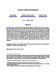
Figure 5: Cycles Required by a Sequence of Packets An initial experiment, presented in Figure 5, shows that the number of cycles required by each packet varies over a wide range: from 1M to 5M cycles in the case of the Terminator 2 clip. However, we observe two distinguishable bands of data, which are highlighted in Figure 5 as blue (black) and green (gray) data points. The blue data points (ranging from roughly 3M to 5M cycles per packet) correspond to those packets that included an EOF marker, while the green points (ranging from roughly 1M to 3M cycles per packet) correspond to packets that do not contain an EOF marker. The explanation for this separation is that whenever a full frame is decoded, it must be dithered—translated to the color map used by the display—and this is a time-consuming process. This is not the case with other packets. Unfortunately, regression analysis does not produce a strong linear relationship between the number of EOF markers in the packet and the number of cycles required by each packet; the R2 value of such a fit is 0.64. The next step is to draw on our experience with frames by factoring size into the model. The difficulty, however, is that it does not make sense to distinguish between packets based on the number of bytes in the packet since all packets are roughly the same size. Instead of bytes-per-packet, one could represent the number of cycles it takes to decode a packet as a function of the number of macroblocks it contains. Such a plot is shown in Figure 6 for Terminator 2, where EOF packets and non-EOF packets show up in separate bands. This example is quite promising, in that the processing required for both EOF and non-EOF packets seems to grow linearly in the number of macroblocks contained in the packet. The linear regression confirms this for non-EOF packets ( R2 = 0:94), but not so strongly for the EOF packets (R2 = 0:78). Focusing on the non-EOF points in Figure 6, we observe a change in slope at about 100 macroblocks. (This change is more pronounced for other videos, and shows up better for Terminator 2 when only a subset of the data points are plotted.) This can be explained by macroblock types: I and P-blocks tend to be larger than the B-block, and so fewer 6

6e+06 0 EOF 1 EOF 5e+06

Packet decode cycles

4e+06

3e+06

2e+06

1e+06

0

50

100

150 Blocks in packet

200

250

300

Figure 6: Decoding Time as a Function of Number of Macroblocks of them fit in a single packet (on the order of 25-100), while many more B-blocks fit in a network packet (on the order of 100 to 250). Figure 7 seems to confirm this hunch by distinguishing between the macroblocks types in the non-EOF band from Figure 6. The question, then, is what happens when we factor block type into the regression? Figure 8 shows the linear fit for just I-blocks, with the number of I-blocks in the packet as the independent variable. The result is disappointing, and in fact, the R2 value is only 0.84. The other block types yield similar results. The problem is that the relationship between the number of blocks and bytes has changed from before since we have lost the invariant that there is a fixed number of bytes in the packet; now the I-blocks in the packet span a variable number of bytes. We also tried the same analysis using bytes rather than blocks, but the results were no better; e.g., I-block cycles as a function of I-block bytes resulted in R2 = 0:85. Trying bytes-per-block yielded similarly disappointing results. Stepping back for a moment, the important thing to remember is that packets carry fragments of frames. We have seen that there is a linear model of cycles-per-frame as a function of bytes-per-frame. To construct a model for cyclesper-fragment based on this relation, we might assume that if we know what fraction of the frame a fragment represents, then it should take that same fraction of the frame processing time to process the fragment. That is, processing half a frame should take half as long as processing the whole frame. With this assumption, and given the linear model for predicting cycles-per-frame, we can model cycles-per-packet as follows. First, let F denote the fraction of the frame carried by this packet. Second, for each fragment in the packet, multiply the bytes in the fragment by 1=F to approximate the number of bytes in the frame. Third, plug this result into the predictor for frames, as defined in Section 3.1, to find the cycles-per-frame. Finally, multiply this result by F to find the cycles required for the fragment. The predicted cycles for the packet will be the sum of the cycles required for all the fragments in the packet. This only begs the question, though, since we need to know the fraction of the frame we’re working on. Fortunately, there is a roughly constant number of macroblocks per frame for a particular video, and so the fraction of a frame contained in a given fragment is related to the number of macroblocks it contains. Applying simple algebra to this reasoning, we find that the cycles for a frame fragment should be a linear model of two independent variables: the number of bytes in the fragment and the number of macroblocks in the fragment. We tested the above reasoning by checking for a linear correlation between the numbers and lengths of each type of macroblock in a packet (the independent variables) and the corresponding cycles to process blocks of that type

7

6e+06 P packets I packets B packets 5e+06

Packet decode cycles

4e+06

3e+06

2e+06

1e+06

0

50

100

150 Blocks in packet

200

250

300

Figure 7: Distinguishing between Macroblock Types (the dependent variable). As we had hoped, regression analysis for each block type resulted in excellent linear fits. Figure 9 shows the resulting regression curves for all four block types. The regression coefficients confirm the visual observations, with R2 values of 0.98 to 0.99 for all four types. At this point we believe that we have isolated all the important factors in an analysis of packet decode time: EOF versus non-EOF, macroblock types, and number of blocks and bytes for each type. To complete the analysis, we constructed a composite model for cycles-per-packet as a linear combination of these factors. The resulting regression coefficient was a very promising 0.97. However, since the sum of the lengths of all macroblocks in a packet is approximately equal to the packet length, which is fixed, we suspect that the length factor is no longer as important. A model that includes only EOF markers and number of macroblocks by type, but omits the length variable, produces an R2 of 0.96.

8

I.cyc 10^6 1.5*10^6 2*10^6 2.5*10^6 3*10^6 5*10^5 0

• • • •• • • • • • ••• • • • •• •• • • • •• • •••••••••••• • •• • • • ••• • • • • •••••••••••• ••••• • •• •• • • •••••••••••••••••••••••• ••• ••• • • • • ••• • • • • • • • • • •••••••••••••••••••••••••••••• • • • • • •••••••••••••••••••• ••••••• • • • • • • •• • ••••••••••••••••••••••••••••••••••••••••••••••••• •••••• • •• •• • • • • • • • • • • • • • ••••••••••••••••••••••••••••••••••••••••••••• • • • • •••••••••••••••••••••••••••••••••••••••• • • • ••• •••• • • • • • • • • • • • • • •••••••••••• • • •••• ••••• • •••••••••••••••••••••••• •••••••••••••••••••••••••••••• •• • • •••••••••••••••••• ••••••••••••••••••••••••••••••••••••••••••• •••••• •• ••••• •• • • ••••••• •••••••••••••••• ••••••••••••• • • • • • • • • • • • • • • • •• • • • • • • • • • • • • • • • • • • •• • • • • • • • ••••••••• ••••••• ••••••••••••••••••••••••••••••••• •••• • ••••••••••••••••••• • ••••••••••••••••••••••••••••••••••• •••••••••••••••• • •••••••••••••••••••••••••••••••••••••••••••••••••••••••••••••••••••••••••••••••••• ••••• • •• • ••••••••••••••••• ••• • • • • • • • • • • • • • • • •• • • • • • • • • • • • • •• • • • • • •• •• • • • • • • • • • • • • •• • • ••• •••••••••••••••••••••••••••••••••••••••••••••••••••••••••••••••••••••••••••••••••••••• •••• • •• •••••••• •• • •••••••••• •• • •• • •••••••••••••••••••••••••••••••••••••••••••••••••••••••••••••••••••••••••••••••••••••••••• • • • ••••••••••••••••••••••••••••••••••••••••••••••••• •••••••• • ••••••••••• •••••••••••••••••••••••••••••••• •••••••••••••••••••••••••• •••••••• •• • •••••••••••••••••••••••••••••••••• •••••••••••••••••••••••••••••••••••••••••••• • ••••••••••••••• •••• • • • • • • •••••••••• •• • • • • • • •• • • •• • •• • • • ••••••••• • • • •• • • • •• • • • • •••••• ••••••• •••••••• •••• •••••• ••••••• •• •••• •••••••••••••••• •••••••••••• •••••• • ••• ••••• • ••• • ••• •••••• •••••••••• •••• •• ••••• •• •• •• •••••••• •• •••••• ••••••• • • • •• • •• 0

10^6

2*10^6

3*10^6 Fitted: I.blk

•

•

•

•

•

4*10^6

5*10^6

6*10^6

•

•• • • • •• •• •••• • • • •••••••••••••• •• • • • • ••• •• •••• ••• •• • • • •••••••••••••••••••••••••••• •• • • •••••••••••••••••••••••••••••••••••• • •••••••••••••••••••••••••••• ••• • •••••••••••••• •••••••• ••• •••••••••••••••••••••••••••••••• • •••••••••••••••••••••••••••••••••••••••• • • •••••••••••••••••••••••••••••••••••••••••••••••••••••••••• •• • • • • • • • • • •• • • • • • • • • • • • • ••••••••••••••••••••••••••••••••••••••••••••••••••••••• ••••••••••••••••••••• ••••••••••••••••••••• • ••••••••••••••••••••• ••••••••••••••••••••••••••••••••••••• • ••••••••••••••••••••••••••••••••••••••• • • • • • • • • • • •••••••••••••••••••••••••••••••••••••• •••••••••••••••••••••••••••••••••••••••••••••••••••••••••••• • •••••••••••••••••••••••••••••••••••••••••••• ••••••••••••••••••••••••••••••••••••••• ••••••••••••••••••••••••••••••••••••••••••••••••••••••••••••••••• • ••••••••••• • ••••••••••••••••• • •••••••••••••••••••••••••••••••••••• •• •••••••••••••••••••••••• • • • ••••••••••••••••••••• ••••••••••••••••••••••••••• • • • • • • • • • ••••••••••• •••••••••••••••• •••••••••• ••••••••

•

0

4*10^6

0

•

•• • • • • •• • • • • ••• •• ••• • • • • • • • • • • • •• •• • ••• •••• •••••••••• ••••••••• • • • • • • • • • • • • • • ••• • •• • • •• •••••• ••••• •••••••••••••••••••••••••••••• •••••• •• • • •••••••••••• •••••••••••••••••• ••••••••••••• •••••• •••••••••••••••••• •• ••••••••••••••••••••••••••••••••••••••••••••••••••••••••••••••••••••••••••••••••••••••••• •••• • • • • • •••••••••••••••••••••••••••••••••••••••• ••• • ••••••••••••••• • • • • • • • • • • • • • • • • • • • • • • • • • • • • • • • • • • • • • • • • • • • ••••••••••••••••••••••••••••••••••••••••••••••••••••••••••••••••••••••••••••••••••••••••••••••••• • • ••• •• ••••••••••••••••••••••••••••••••••• ••••••••••••••••••••••••••••••••••••••••••••••••••••••••••••••••••••••••••• • • •••••••••••••••••••••••••••••••••• •••••••••••••••••••••••••• •••••••••••••• • •••••••••••• ••••••••••• •••••••••••••••••••••••••••••••••••••••••••••••••••••••• • •••••••••••• ••••••••••••••••••••••••••••••••••••••••••••••••• ••• • • • • ••••••••••••• ••••••••••••••••••••••••••••••••••••• ••••••••••••••••• •• • ••••••••••••••••••••••••••••••••••• • • • • • • • • • • • • • • • • • •••••••••••••••••••••••••••••••••••••••••••••••••••••••••••••••••••••••••••••••••••••••• •••••••••••••••••••••••••••••••••••••••••• ••••••••••••••• •• ••••••••••••••••••••• ••••••••••••••••••••••••••• •••••••• • ••••••••••••••••••••••••••••••••••••••••••• • •••••••••• ••••••• •••••••••••••••••••••••••••••••••••••••••••••••• ••••••••••••••••••••••••••••• ••••••••••••••••••••••••••••••••••••••••••••••••••••••••••• • • • • • • •••••••••••••••••••••••••••••• •• • ••••••••••• •• • ••••••••••••••••••••••••••••••••• •••••••••••••••••••••••• • •• •• ••• • ••••••• ••••••••••••••••••••• •••••••••••••••••••••• • • ••••••••••••••••••••• ••••••••••••••••••• • • • •• • • ••••

10^6

2*10^6 Fitted: B.blk + B.byte

3*10^6

0

5*10^5

Bi.cyc 10^6

1.5*10^6

• • • •

• •

•

•• ••• • •• • • • ••• • ••••• •••• • • • • •••••• • •• • ••••••••••••••• ••••••• •••••••••• ••••••••••••••••••• • • • • • • • • • ••••••••••••••••••• •• • • • • • • • • ••••••••••• • • •••••••••••••••••••• • ••••••••••••••••••• ••••••••••••••••••••••••••••••• • ••••••••• ••• •••• •••••••••••••••• • •••• •• •• • • ••• 5*10^5

10^6 Fitted: Bi.blk + Bi.byte

1.5*10^6

•

0

10^6

2*10^6 3*10^6 Fitted: I.blk + I.byte

2*10^6

• •

•

3*10^6

•

P.cyc 2*10^6

•

10^6

• •• • • •• • • •• • • •••••••• ••• • •• • • • • •••••• • • •••••• •• •• •• ••••••••••••••••• •••••• • • • • • • •• • • • •• • •••••••••••••••••••••••• ••••••••••••••••••••••••••• • • •• ••••••••••••••••••••••••••••• •• • • •• • •••••••••••••••••••••••••••••••••••••••••••••••••••••••• •• • • • • ••••• •••••••••••••••••••••••••••••••••••••••••• • •••••••••• • •••• ••••••••••••••••• • •• ••••••••••••• ••••• ••• ••••••••••••••• • • •••••••••••••••••• • • • • • ••••••••••••••••••••••••••••••• •• • ••••••••••••••••••••••• •••• • •• •••• •••••••• ••••••••••• •••••••• ••••••••••• •••••••• ••••• ••••• •••••••• •• •• ••••• ••••••• •••••••••• •••••••••••••••• ••••• ••••••••••••••••••• •••••••••• •••••••••••• •••• ••••••••••• •• • •• ••• ••••••• ••••••••••••••••••••••••••••••••••••• •••••• • • • •• • • • • • • • • • • • • • • • ••••••••••••••••••••••••• •••••• • • •••••• •••••••••••••••••••••• ••••••••••••• • • • • • •••••••••••• • •• •••••••••••••••••••••••••••••••••••••••••••••• • • •••••••••••••••••••••••••••••••••••••••••••••••••••••••••••••• • • •••••••••••••••••••••••••• •••••• ••••••••••••••••••••••• •••••••••••••••• •••• ••• •••••••••••••••••••••••••••• • • • • • • • • • • • • • • • • • •• ••••••• ••• ••••••••• ••• ••••••••••••••••• •••••••• •• ••••••• ••••••••••••••• ••••••••••••••••••••• ••••• •••••• ••• ••••• •••••••••• •••••• •••••••••• ••••• ••••• •• ••••••••••••••••••••• •••• •••• •••• •••••••••••••••• ••••••• •••• •••• •• •••••••• • • • •• •• ••• • • • • ••••••

0

0

5*10^5

I.cyc 10^6 1.5*10^6 2*10^6 2.5*10^6 3*10^6

0

10^6

B.cyc 2*10^6

3*10^6

•

2*10^6

Figure 8: Cycles for I-Blocks as a Function of the Number of Blocks

4*10^6

0

10^6

2*10^6 Fitted: P.blk + P.byte

Figure 9: Regression Analysis based on Macroblock Types

9

3*10^6

• •

4*10^6

4 Estimators We now describe and evaluate seven different predictors, based on the observations made in the previous section. We also explain how such predictors can be implemented in an OS like Scout.

4.1 Packet Preprocessing Predicting how much processing time a packet is going to require—before actually starting to process the packet—is tricky. This is especially true if the predictor needs detailed information about the contents of the packet, such as how many I-blocks it contains. Fortunately, Scout’s path architecture already includes a mechanism that addresses this problem. As briefly describe in Section 2.2, Scout classifies each incoming packet to determine the path to which it belongs. This involves inspecting various header fields in the packet, such as ETH’s type field, IP’s protnum field, UDP’s port fields, and so on. Although the details are beyond the scope of this paper, in essence classification is accomplished incrementally, with each module (protocol) making a partial classification decision using module-specific information. For example, the IP module interprets just the IP header. The classification process is considered successful if a unique path is identified, in which case Scout places the packet on that path’s source queue. Packet classification can be viewed as a form of preprocessing that takes place when the packet arrives, and as such, it is possible to do other kinds of preprocessing as well. In our case, the MPEG-specific classifier inspects its header to learn about the number and type of macroblocks contained in that packet. It then uses this information to compute an estimate for the packet according to one of the predictors given in the next subsection. This estimator can be viewed as a derived attribute of the packet, one that Scout can then use to schedule the packet for execution.

4.2 Predictors We implemented seven predictors, as summarized below. The first three operate at the frame level (predicting the number of cycles required for each frame) and the last four operate at the packet level (predicting the number of cycles required for each packet). Within each set, the predictors range from simple averages to more complex estimators based on the statistical models discussed in Section 3. Building efficient estimators is more complicated than implementing the models described in Section 3. The first problem is that the models were applied off-line, with all the data available to them a priori. In the case of predicting, we have to incrementally estimate the number of cycles needed based on the frames or packets processed so far. The second problem is that the models used in Section 3 are based on the least squares algorithm, and even if we apply this algorithm incrementally, it is too computationally expensive for our purposes; we have a budget of only a few cycles per frame (packet) to estimate how long the the frame (packet) will require to be decoded. Thus, we will have to design estimators that approximate the models we have developed. FRAME AVG: Predicts processing time for next frame based on the average processing time required by all previous frames that are part of this video stream. FRAME TYPE: Same as FRAME AVG except it distinguishes among frames based on frame type, that is, it maintains three separate averages for each video stream. FRAME TYPE LEN: Approximates the model described at the end of Section 3.1. Keeps the same per-type average as does FRAME TYPE, but adjusts this prediction to account for the slope of the cycles-per-byte line. The code fragment that implements FRAME TYPE LEN is given in the appendix. PACKET AVG: Predicts processing time for next packet based on the average processing time required by all previous packets that are part of this video stream. PACKET EOF: Same as PACKET AVG except it distinguishes among packets based on the number of EOFs contained in the packet. For most video streams, this means maintaining two averages: one for packets with no EOF markers and another for packets with one EOF marker. 10

PACKET EOF TYPE: Tracks the average number of cycles required for each macroblock type. For each type of macroblock in a given packet, multiplies the number of macroblocks of that type contained in the packet times the corresponding average. The final prediction is given by the sum of these values, plus the average dithering time if EOF is present. PACKET EOF TYPE LEN: Approximates the composite model described at the end of Section 3.2. Similar to FRAME TYPE LEN except defined in terms of blocks-per-packet rather than bytes-per-frame. The code fragment that implements PACKET EOF TYPE LEN is given in the appendix.

4.3 Evaluation We ran the seven predictors on the videos identified in Table 1. This section evaluates the accuracy of the predictors on this sample set. For each frame (packet) processed by MPEG, we calculated the prediction error to be the difference between the number of cycles predicted by the corresponding estimator, and the number of cycles actually required to decode the frame (packet). The graphs and tables presented in this section report this prediction error in one form or another. 4.3.1 Frame Predictors Beginning with the frame predictors, we found that the simple average (FRAME AVG) did very poorly, the predictor based on frame type (FRAME TYPE) did only marginally better, and the predictor based on both frame type and length (FRAME TYPE LEN) did very well. Figure 10 illustrates visually how well these three predictors performed on one representative video: Terminator 2. In this figure, there is one scatter plot for each predictor, where every data point records the prediction error for one frame processed by that predict or. That is, a data point at 0 on the y axis indicates that the prediction for the corresponding frame was exactly right, a data point at 106 on the y axis indicates that the prediction for the corresponding frame was 1M cycles too low, and a data point at ?106 on the y axis indicates that the prediction for the corresponding frame was 1M cycles too high. One interesting observation is that the plot of the error for FRAME AVG has the same structure as the frame decode times shown in Figure 2. We examined the behavior of FRAME TYPE LEN more closely by plotting the distribution of the prediction error. A histogram for Terminator 2 is given in Figure 11. As this Figure illustrates, the prediction error is normally distributed about 0, the perfect prediction. As a final evaluation of our frame predictors, we applied each of them to all six videos. The results for the best predictor—FRAME TYPE LEN—are presented in Table 2. This table shows both the absolute and relative errors measured for each of the six videos. Video Neptune RedsNightmare Canyon Terminator 2 Road Warrior Mandelbrot

Absolute Error % w/in 1ms % w/in 10ms 72 99.7 67 99.0 99 100 56 99.7 63 99.6 16 86

% w/in 5% 80 60 75 75 81 74

Relative Error % w/in 10% % w/in 25% 97 99.4 84 97 94 99.3 96 99.7 96 99.6 88 97

Table 2: Absolute and Relative Error for FRAME TYPE LEN Predictor In the case of the absolute error, the table reports the percentage of frames that MPEG actually decoded within 1ms and 10ms of the predicted time, as measured on a 300MHz Alpha (thus, 1ms = 300,000 cycles and 10ms = 3M cycles). We chose 1ms because it represents the minimum practical granularity for a scheduling algorithm; predicting decoding time any more accurately would be of little value. We chose 10ms because it corresponds to the granularity that scheduling decision are made in practice, and as such, represents a reasonable target upper bound for the absolute

11

1.5*10^7 Decode cycles 0 5*10^6

•

• • •

• •

• •

• • • • •• •• • • ••• • •••••• • •••••••• • • •• •• ••• • • • ••• ••• • • •• ••• • •••• ••• •• ••• • ••••••• •• •••••••••••••••••••••• •••• •••••••••••••••••••••••••••••••••••••••••••• ••••••••••••••••• •••••••••••••••••• ••••••• •• •••• •••••••••••• • • • •••• ••••••••••••••••••••••••• ••• ••••• • • ••• ••••••••••••••••••••••••••••••••••••••••••••••••••••••••••••••••••••••••••••••••••••••••••••••••••••••••••••••••••••••••••••••••••••••••••••••••••••••••••••••••••••••••••••••••••••••••••••••••••••••••••••••••••••••••••••••••••••••••••••••••••••••••••••••••••••••••••••••••••••••••••••••••••••••••••••••••••••••••••••••••••••••••••••••••••••••••••••••••••••••••••••••••••••••••••••••••••••••••••••••••••••••••••••••••••••••••••••••••••••••••••••••••••••••••••••••••••• • • ••••••••••••••••••••••••••••••••••••••••••••••••••••••••••••••••••••••••••••••••••••••••••••••••••••••••••••••••••••••••••••••••••••••••••••••••••••••••••••••••••••••••••••••••••••••••••••••••••••••••••••••••••••••••••••••••••••••••••••••••••••••••••••••••••••••••••••••••••••••••••••••••••••••••••••••••••••••••••••••••••••••••••••••••••••••••••••••••••••••••••••••••••••••••••••••••••••••••••••••••••••••••••••••••••••••••••••••••••••••••••••••••••••••••••••••••••••••••••••••••••••••••••••••••••••••••••••••••••••••••••••••••••••••• • • • • • •• •• • •••••••••••••••••••••••••••••••••••••••••••••••••••••••••••••••••••••••••••••••••••••••••••••••••••••••••••••••••••••••••••••••••••••••••••••••••••••••••••••••••••••••••••••••••••••••••••••••• ••••••••••••••••••••••••••••••••••••••••••••••••••••••••••••••••••••••••••••••••••••••••••••••••••••••••••••••••••••••••••••••••••••••••••••••••••••••••••••••••••••••••••••••••••••••••••••••••••••••••••••••••••••••••••••••••••••••••••••••••••••••••••••••••••••• ••• ••••••••••• • ••• •• •• ••••• • •• • ••• •• •••••• ••• •• ••••••••• •••••• • • ••••••• •••• •• • •••••••• ••••••• •••• •••••••••••• •• ••••••••••• •• • • • •• • • •• • •••• •• •• • • • • •••• • • • •• •• • ••• • • ••••• • • ••• ••• • ••••• ••• ••••• • • • ••• • •• •• • •• •• • • • • • •

1000

2000 FRAME_AVG

3000

4000

0

1000

2000 FRAME_TYPE

3000

4000

• •

10^7

1.5*10^7

0

• •

10^7

•• • • • • • ••• • • •• • • • • • • •• • •••• • • • • • • •• ••• ••••• •••• •••• • • •••••••••••• • • • • • • • •• •• • •• •• ••• ••• • • •• •••••••• • •• •• • • • • •• • • •• • • • •••• •• • •••••••• •• •• •• • • ••••••••••••••••••••• •••••••••••••••••••••••••••• ••••••••••• •••••••• •••• • ••••••• •••••• ••• •••••••••••• •••• • ••••• ••• •• ••• ••••••••••••••• ••••• • • • • • • ••• • •• • ••• •• •••• • ••• • • • •••• ••• • • • •••• • • • • •••••• •••• • • ••••••••••••• •••••••• •••••••••• ••• • ••••••••••• •••••••••••••••••••••••••••••••••••••••••••••••••••••••••••••••• •••••••••••••• ••••••••••••••••••••••••• •••••••••••• •••••••••••••••••••••••••••••••••••• ••••••••• ••••••••••••• ••••••••• • • •••••• ••••••• •••••••••••••••• • • •••• ••••••••••• ••••••••••••••••••••••••• ••••••••••• •••••••••••• ••••••••••••• ••••• •••• ••••••••• ••• •••••• ••••••••• ••• ••• • • • • • • • • • • • • • • • • • • • • • • • • • • • • • • • • • • • • • • • • • •• • • •• ••• • •••••• •• •• • •••••• •••• •• • •• •• • •• ••• •• ••••••• ••• •• • • •• • • ••• •••••••••••••••••••• •• • ••••••• • •••••••••••• •• •• •••• ••••••••••••••••••• ••• ••••••• • •••• •• • ••••••••••••••• •••••• ••••••••••••• ••••••••• ••• ••••••••••••••••••• •••• •••••••••••••••••••••• • • •• •• • •• •••••••••••••• ••••• •• • •••• •••• •••••••• •• •• • • ••••••••• ••• • • • ••••••••••••••••• ••• • •••• •••• •••••• •• • ••••••••••••••••• ••••••••••••••••••••••••••••••••••••••••••••••••••••••••••••••••••••••••••••••••••••••••••••••••••••••••••••••••••••••• ••••••••••••••••••••••••••••••••••••••••••••••••••••••••••••••• •••••••••••••••••••••••••••••••••••••••••••••••••••••••••••••••••••••••••••••••••••••••••••••••••••••••••••••••••••••••• • • • • • •• • • • •• •• • • •• • • •••• • •• • •••••• • •• •• • • • • •••••••••••••••••••••••••••••••••••••••••••••••••••••••••••••••••••••••••••••••••••••••••••••••••••••••••••••••••••••••••••••••••••••••••••••••••••••••••••••••••••••••••••••••••••••••••••••••••••••••••••••••••••••••••••••••••••••••••••••••••••••••••••••••••••••••••••••••••••••••••••••••••••••••••••••••••••••••••••••••••••••••••••••••••••••••••••••••••••••••••••••••••••••••••••••••••••••••••••••••••••••••••••••••••••••••••••••••••••••••••••••••••••••••••••••••••••••••••••••••••••••••••••••••••••••••••••••••••••••••••••••••••••••••••••••••••••••••••••••••••••••••••••••••••• •••••••••••••••••••••• ••••••••••••••• •• • •••••••••••••• • • • • •••••• •••••• • •• • • •• • •• •••••••••• •• • •• •• •• •• ••••••••••••••••••••••••••••••••••••••••••••••••••••••••••••••••••••••••••••••••••••••••••••••• •••••• •• • •••• •••••••• •• ••••••••••••••• •••• •••••••••••••••••••••• ••••• • •••• •••••••••••••••• ••••• • • • • • • • • • ••• • • • • • • • •

-5*10^6

1.5*10^7 10^7 Decode cycles 5*10^6 0 -5*10^6

•

-5*10^6

0

Decode cycles 5*10^6

•

••• • • •• •• • • ••••• • • • •••••• •• •• •• • ••• •••• •• •• ••••••••• •• •• •• • ••••••••••••••••••••• ••••• ••••• •• • ••••••••• • • •••••• • ••••••••••• •• •• • •••••• •• • • • •••••• •••••• • ••••••••••••••••••••••••••••••••••••••••••••••••••••••••••••••••••••••••••••••••••••••••••••••••••••••••••••••••••••••••••••••••••••••••••••••••••••••••••••••••••••••••••••••••••••••••••••••••••••••••••••••••••••••••••••••••••••••••••••••••••••••••••••••••••••••••••••••••••••••••••••••••••••••••••••••••••••••••••••••••••••••••••••••••••••••••••••••••••••••••••••••••••••••••••••••••••••••••••••••••••••••••••••••••••••••••••••••••••••••••••••••••••••••••••••••••••••••••••••••••••••••••••••••••••••••••••••••••••••••••••••••••••••••••••••••••••••••••••••••••••••••••••••••••••••••••••••••••••••••••••••••••••••••••••••••••••••••••••••••••••••••••••••••••••••••••••••••••••••••••••••••••••••••••••••••••••••••••••••••••••••••••••••••••••• • • • • ••• • • • •• • • • • • •• • • ••••••••••••••••••••••••••••••••••••• ••••••••••••••••••••••••••••••••••••• •••• ••••••••••••••••••••••••••••••••••••••••••••••• ••••••••••••••••••••••••••••••••••••••• •••••••••••••••••• •••••••••••••••••••••••••••••••••••••••••••••••••••••••••••••••••••••••••••••••••••••••••••••••••••••••• ••••••••••••••••••••• • • • • • •• •• •• •• • •••••••••• • • •• •• •• • • •• • • • • • • • • • 0

1000

2000 3000 FRAME_TYPE_LEN

4000

Figure 10: Error Plots for Frame Predictors error the scheduler can tolerate. As illustrated in Table 2, 56-72% of the frames are predicted to within 1ms for all but the Mendelbrot video, and (again with the exception of Mandelbrot) virtually all the frames are predicted to within 10ms of the actual time required. In the case of Mandelbrot, which is so complex that it can be played at a rate of only 2 fps on a 300MHz Alpha, the absolute errors are large, but the relative errors are quite good. For example, 88% of the Mandelbrot frames are predicted to within 10% of the time it took to decode that Mandelbrot frame.

12

400 300 200 100 0 -2*10^6

-10^6

0 Error in cycles

10^6

2*10^6

Figure 11: Histogram of Errors for FRAME TYPE LEN

13

4.3.2 Packet Predictors

4*10^6

•

0

5000

10000

Decode cycles 10^6 2*10^6 0 -10^6

• • • •• • • • • •••••••••••• ••••• •• ••••••••••••• • • •• • • • • •••••••• • •••••••••••••••• ••••••• •••• ••••••••••• •••••••••••••••••••••••••••••••• • ••• ••• •• ••• • • ••• • • • • • • •••••• •• • •••• • • • • ••• • •• • • •• • • •• • • ••••••••••••••••••••••••••••••••••••••••••••••••••••••••••••••••••••••••••••••••••••••••••••••••••••••••••••••••••••••••••••••••••••••••••••••••••••••••••••••••••••••••••••••••••••••••••• •••••• •••••••••••••• ••• ••••••••••••••••••• ••••••••••••••••••••••• •• ••••••••••••••••••••••••••••••••••••• ••••••••••• • • ••••••••••••••••••••••••• ••• •••••••• ••••••••••••••••••••••••••••••••••••••••••••••••••••••••••••••••••••••••••••••••••••••••••••••••••••••••••••••••••••••••••••• ••••••••••••••••••••••••••••••••••••••••••••••••••••••••••••••••••••••••••••••••••••••••••••••••••••••••••••••••••••••••••••••••••••••••••••••••••••••••••••••••••••••••••••••••••••••••••••••••••••••••••••••••••••••••••••••••••••••••••••••••••••••••••••••••••••••••••••••••••••••••••••••••••••• •••••• • • • •• ••• • •••••••••• • •• •• • •••••• ••••••• •••••• • •• ••• •• •••••••••• • •••••• ••••••• • • •••• •••••••• ••••••• •• •••••• •••••••••••••••••••••••••••••••••••••••••••••••••••••••••••••••••••••••••••••••••••••••••••••••••••••••••••••••••••••••••••••••••••••••••••••••••••••••••••••••••••••••••••••••••••••••••••••••••••••••••••••••••••••••••••••••••••••••••••••••••••••••••••••••••••••••••••••••••••••••••••••••••••••••••••••••••••••••••••••••••••••••••••••••••••••••••••••••••••••••••••••••••••••••••••••••••••••••••••••••••••••••••••••••••••••••••••••••••••••••••••••••••••••••••••••••••••••••• • • •••••••••• •••••••••••••••••••••••••••••••••••••••••••••••••••••••••••••••••••••••••••••••••••••••••••••••••••••••••••••••• ••••••••••••••••••••••••••••••••••••••••••••••••••••••••••••••••••••••••••••••••••••••••••••••••••••••••••••••••••••••••••••••••••••••••••••••••••••••••••••••••••••••••••••••••••••••••••••••• ••••••••• ••••••••••••••••••••••••••••••••••••••••••••••••••••••••••••••••••••••••••••••••••••••••••••••••••••••••••••••••••••••••••••••••••••••••••••••••••••••••••••••••••••••••••••••••••••••••••••••••••••••••• ••••••••••••••••••••••• •••••••••••••••••••••••••••••••••••••••••••••••••••• ••• ••••••••••••••••••••••••••••••••••••••••••••••••••••••••••••••••••••••••••••••••••••••••••••••••••••••••••••••••••••••••••••••••••••••••••••••••••••••••••••••••••••••••••••••••••••••••••••••••••••••••••••••••••••••••••••••••••••••••••••••••••••• •••••••••••••••••••••••••••••••••••••••••••••••••••••••••••••••••••••••••••••••••••••••••••••••••••••••••••••••••••••••••••••••••••••••••••••••••••••••••••••••••••••••••••••••••••••••••••••••••••••••••••••••••••••• ••••••••••••••••••••••••••••••••••••••••••••••••••••••••••••••••••••••••••••••••••••••••••••••••••••••••••••••••••••••••••••••••••••••••••••••••••••••••••••••••••••••••••••••••••••••••••••••••••••••••••••••••••••••••••••••••••••••••••••••••••••••••••••••••••••••••••••••••••••••••••••••••••••••••••••••••••••••••••••••••••••••••••••••••••••••••••••••••••••••••••••••••••••••••••••••••••••••••••••••••••••••••••••••••••••••••••••••••••••••••••••••••••••••••••••••••••••••••••••••••••••••••• ••• ••••••••••••••••••• ••••••••••••••••• ••••••• •••••••••• •••••••••••••••••••••••••••••••••••••••••••••••••••••••••••••••••••••••••••••••••••••••••••••••••••••••••••••••••••••••••••••••••••••••••••••••••••••••••••••••••••••••••••••••••••••••••••••••••••••••••••••••••••••••••••••••••••••••••••••••••••••••••••••••••••••••••••••••••••••••••••••••••••••••••••••••••••••••••• •••••• ••••••• •••••••••••••• •••••• •• •••••••••••••••••••••••••••••••••••••• ••••••••••••••••••••••••••••••••••••••••••••••••••••••••••••••••••••••••••••••••••••••••••••••••• ••• •••••••••••••••••••••••••••••• •••••••••••••••••••••••••••••••••••••••••••••••••••••••••••••••••••••••••••••••••••••••••••• ••••••••• ••••••••••••••••••••••••••••••• •••••••• • • • •• • • •••••••••• ••••••• •••••••••••••••••••••••••••••••••••••••••••••••••••• •••••••••••••••••••••••••••••••••••••••••••••••••••••••••••••••••••••• ••••••••••••• •••••••• ••••••••••• ••• • ••••••• ••••••• ••••••••••••••••••••••••• •••••••••••••••••••••• •••••••••••••••••••••••••••••••••••••••••••••••••••••••••••••••••••••••••••••••••••••••••••••••••••••••••••••••••••••••••••••••••••••••••••••••••••••••••••••••••••••••••••••••••••••••••••••••••••••••••••••••••••••• •••••••••••••••••••••••••••••••••••••••••••••••••••••••••••••••••••••••••••••••••••••••••••••••••••••••••••••••••••••••••••••••••••• ••••••••••• ••••••••••••••••••••••••• •••••••••••••••••••••••••••••••••••••••• •••••• ••••••••••••••••• ••••••••••••••••••••••••••••••••••••••••••••••••••••••••••••••• •• ••• •••••••••••••••• ••••••••••••••••• •••••••••••••••••••••••••••••••••••••••••••••••••••••••••••••••••••••••••••••••••••••••••••••••••••••••••••••••••••••••••••••••••••••••••••••••••••••••••••••••••••••••••••••••••••••••••••••••••••••••••••••••••••••••••••••••••••••••••••••••••••••••••••••••••••••••••••••••••••••••••••••••••••••••••••••••••••••••••••••••••••••••••••••••••••••••••••••••••••••••••••••••••••••••••••••••••••••••••••••••••••••••••••••••••••••••••••••••••••••••••••••••••••••••••••••••••••••••••••••••••••••••••••••••••••••••••••••••••••••••••••••••••••••••••••••••••••••••••••••••••••••••••••••••••••••••••••••••••• • ••• • • • •• • • • • • • • • • • • •••••••••••••••••••••••••••••••••••••••••••••••••••••••••••••••••••••••••••••••••••••••••••••••••••••••••••••••••••••••••••••••••••••••••••••••••••••••••••••••••••••••••••••••••••••••••••••••••••••••••••••••••••••••••••••••••••••••••••••••••••••••••••••••••••••••••••••••••••••••••••••••••••••••••••••••••••••••••••••••••••••••••••••••••••••••••••••••••••••••••••••••••••••••••••••••••••••••••••••••••••••••••••••••••••••••••••••••••••••••••••••••••••••••••••••••••••••••••••••••••••••••••••••••••••••••••••••••••••••••••••••••••••••••••••••••••••••••••••••••••••••••••••••••••••••••••••••••••••••••••••••••••••••••••••••••••••••••••••••••••••••• ••••••••••••••••••••••••••••••••••••••••••••••••••••••••••••••••••••••••••••••••••••••••••••••••••••••••••••••••••••••••••••••••••••••••••••••••••••••••••••••••••••••••••••••••••••••••••••••••••••••••••••••••••••••••••••••••••••••••••••••••••••••••••••••••••••••••••••••••••••••••••••••••••••••••••••••••••••••••••••••••••••••••••••••••••••••••••••••••••••••••••••• ••••••••••••••••••••••••••••••••••••••••••••••••••••••••••••••••••••••••••••••••••••••••••••••••••••••••••• ••••••••••••••••••••••••••••••••••••••••••••••••••••••••••••••••••••••••••••••••••••••••••••••••••••••••••••••••••••••••••••••••••••••••••••••••••••••••••••••••••• •••••••• •••••••••••••••••••••••••••••••••••••••••••••••••••••••••••••••••••••••••••••••••••••••••••••••••••••••••••••••••••••••• •••••••••••••••••••••••••••••••••••••••••••••••••••• •••••••••••••• •••••••••• ••••••••••••• ••••••• •••• • ••••••••••••• ••••• •••• • ••••• • ••••• • • • •• •••••••• •••••••••••••••• ••••••••• ••••• ••••• •• ••••••••• • •• •• ••• • • •• • • • •• • • • •

3*10^6

••

•

-2*10^6

-2*10^6 -10^6

0

Decode cycles 10^6 2*10^6 3*10^6 4*10^6

We next turn our attention to the packet predictors. Analogous to Figure 10, Figure 12 plots the errors measured for each of the four packet predictors when applied to Terminator 2. In this case, we see that simple averages work very poorly, and that PACKET EOF TYPE LEN is clearly the best predictor. A histogram of the error distribution for PACKET EOF TYPE LEN is shown in Figure 13, and again we see a normal distribution around 0 prediction error.

15000

•

• •

••

• • •••••• • • •• • •••••••• • ••••• • •••••••••••••••• • • • • ••••••••• •••••••••••••••••••••••••••• •••••••••• •••••••••••••••••••••••••••••••••••••••••••••••• •••••• •• ••••••• • • ••• • • ••• ••• •••• •• • •••• ••• •••• • • • •• • •• •••••••••• •••••••••••• •••• • •• • •• • •• • • • • • • ••• • • ••••••••••••••••••••••••••••••••••••••••••••••••••••••••••••••••••••••••••••••••••••••••••••••••••••••••••••••••••••••••••••••••••••••••••••••••••••••••••••••••••••••••••••••••••••••••••••••••••••••••••••••••••••••••••••••••••••••••••••••••••••• ••••••••••••••••••••••••••••••••••••••••••••••••••• •••••••••••••••••• ••••••••••••••••••••••••••• •••••••••• • • • • • • • • • • • • • • • • • • • • • • • • • • • • • • • • • • • • • • • • • • • • • • • • • • • • • • • • • • • • • • • • • • • • • • • • • • • • • • • • ••• • ••••• •••• •• ••• • •• • •• • ••••• • •• ••••••••••••••• • • ••••• •• •••• ••••• •••••••• • • ••••••••••••• • •••••••••••••••••••••••••••••••••••••••••••••••• ••• •••••••••••••••••••• •••••••••••••••••••••••• •••• •• •••••• •••••••••••••••••••••••••••••••••••••••••••••••••••••••••••••••••••••••••••••••••••••••••••••••••••••••••••••••••••••••••••••••••••••••••••••••••••••••••••••••••••••••••••••••••••••••••••••••••••••••••••••••••••••••••••••••••••••••••••••••••••••••••••••••••••••••••••••••••••••••••••••••••••••••••••••••••••••••••••••••••••••••••••••••••••••••••••••••••••••••••••••••••••• •••••• • ••••••••• ••••••••• •• ••• ••••••••••••••••••••• •••••••• •••••••••••••••••••••••••••••••••••••••••••••••••••••••••••••••••••••••••••••••••••••••••••••••••••••••••••••••••••••••••••••••••••••••••••••••••••••••••••••••••••••••••••••••••••••••••••••••••••••••••••••••••••••••••••••••••••••• •• ••••••• • • •• •• •• ••• • • •• •• •• ••••• •• • • • •••• •• • • • ••• ••••• •••• •• • ••••••••••••••••••••••••••••••••••••••••••••••••••••••••••••••••••••••••••••••••••••••••••••••••••••••••••••••••••••••••••••••••••••••••••••••••••••••••••••••••••••••••••••••••••••••••••••••••••••••••••••••••••••••••••••••••••••••••••••••••••••••••••••••••••••••••••••••••••••••••••••••••••••••••••••••••••••••••••••••••••••••••••••••••••••••••••••••••••••••••••••••••••••••••••••••••••••••••••••••••••••••••••••••••••••••••••••••••••••••••••••••••••••••••••••••••••••••••••••••••••••••••••••••••••••• •••••••••••••••••••••••••••••••••••••••••••••••••••••••••••••••••••••••••••••••••••••••••••••••••••••••••••••••••••••••••••••••••••••••••••••••••••••••••••••••••••••••••••••••••••••••••••••••••••••••••••••••••••••••••••••••••••••••••••••••••••••••••••••••••••••••••••••••••••••••••••••••••••••••••••••••••••••••••••••••••••••••••••••••••••••••••••••••••••• •••••••••••• •••••••• •••••••• •••••••• • ••••••••• • • •••• • •••••••••••••• ••••••• ••• ••••••••••• • ••••••••• ••••• •••••• ••••••••• • • ••• ••• ••••••••••••••••••••••••••••••••••••••••••••••••••••••••••••••••••••••••••••••••••••••••••••••••••••••••••••••••••••••••••••••••••••••••••••••••••••••••••••••••••••••••••••••••••••••••••••••••••••••••••••••••••••••••••••••••••••••••••••••••••••••••••••••••••••••••••••••••••••••••••••••••••••••••••••••••••••••••••••••••••••••••••••••••••••••••••••••••••••••••••••••••••••••••••••••••••••••••••••••••••••••••••••••••••••••••••••••••••••••••••••••••••••••••••••••••••••••••••••••••••••••••••••••••••••••••••••••••••••••••••••••••••••••••••••••••••••••••••••••••••••••••••••••••••••••••••••••••••••••••••••••••••••••••••••••••••••••••••••••••••••••••••••••••••••••••••••••••••••••••••••••• ••••••••••••••••••••••••••••••••••••••••••••••••••••••••••••••••••••••••••••••••••••••••••••••••••••••••••••••••••••••••••••••••••••••••••••••••••••••••••••••••••••••••••••••••••••••••••••••••••••••••••••••••••••••••••••••••••••••••••••••••••••••••••••••••••••••••••••••••••••••••••••••••••••••••••••••••••••••••••••••••••••••••••••••••••••••••••••••••••••••••••••••••••••••••••••••••••••••••••••••••••••••••••••••••••••••••••••••••••••••••••••••••••••••••••••••••••••••••••••••••••••••••••••••••••••••••••••••••••••••••••••••••••••••••••••••••••••••••••••••••••••••••••••••••••••••••••••••••••••••••••••••••••••••••••••••••••••••••••• •••••••••• ••••••••• ••••••• •••••••••••••••••••• •••••• ••••••••••••••••••••••••••••••••••••••••••••••••• • ••••••••••••• ••••••••• •••••••••••••••••••••••••• ••••• •••• •••••••••••••• ••••••••••••••••••••••••••••••••••••••••••••••••••••••••••••••••••••••••••••••••••••••••••••••••••••••••••••••••••••••••••••••••••••••••••••••••••••••••••••••••••••••••••••••••••••••••••••••••••••••••••••••••••••••••••••••••••••••••••••••••••••••••••••••••••••••••••••••••••••••••••••••••••••••••••••••••••••••••••••••••••••••••••••••••••••••••••••••••••••••••••••••••••••••••••• ••••••••••••••••••••••••••••••••••••••••••••••••••••••••••••••••••••••••••••••••••••••••••••••••••••••••••••••••••••••••••••••••••••••••••••••••••••••••••••••••••••••••••••••••••••••••••••••••••••••••••••••••••••••••••••••••••••••••••••••••••••••••••••••••••••••••••••••••••••••••••••••••••••••••••••••••••••••••••••••••••••••••••••••••••••••••••••••••••••••••••••••••••••••••••••••••••••••••••••••••••••••••••••••••••••••••••••••••••••••••••••••••••••••••••••••••••••••••••••••••••••••••••••••••••••••••••••••••••••••••••••••••••••••••••••••••••••••••••••••••••••••••••••••••••••••••••••••••••••••••••••••••••••••••••••••••••••••••••••••••••••••••••••••••••••••••••••• •••••••••••••••••••••••••••••••••••••••••••••••••••••••••••••••••••••••••••••••••••• ••••••••••••••••••••••••••••••••••••••••••••••••••••••••••••••••••••••••••••••••••••••••••••••••••••••••••••••••••••••••••••••••••••••••••••••••••••••••••••••••••••••••••••••••••••••••••••••••••••••••••••••••••••••••••••••••••••••••••••••••••••••••••••••••••••••••••••••••••••••••••••••••••••••••••••••••••••••••••••••••••••••••••••••••••••••••••••••••••••••••••••••••••••••••••••••••••••••••• ••••••••••••• •••••••••••• ••• •• •••••••• •••• • • •••••••• •••• •••••••••• •••••••• • ••••••••••••• •••• ••••• ••••••••••••••••••••••••• •••••••• •••••••••••••••••• •• ••• •• ••••• •• •• •• • •• •• •• • • • • •• • • • •• • •• •• •• •• • •••• •• • • •• • ••• • • • • ••• •••••• ••••••• ••••• ••••• •••• • • •• • • • •• • •• •• ••• • • ••••••• • • •• 0

5000

• •

10000

15000

PACKET_EOF

•

• •

• • • •• •• • • • •••••••••••••••••••••••••••••••••••••••••••••••••••••••••••••••••••••••••••••••••••••••••••••••••••••••••••••••••••••••••••••••••••••••••••••••••••••••••••••••••••••••••••••••••••••••••••••••••••• ••••••••••• •••••••• •••••••••• •••••••••••••••••••••••••••••• ••••••••••••••••••• ••• •••••••••••••••••• •••••••••••••••••••• •••••••••••• •••••••••••••••••••••••••••••••••••••••••••••••••••••••••••••••••••••••••••••••••••••••••••••••••••••••••••••••••••••••••••••••••••••••••••••••••••••••••••••••••••••••••••••••••••••••••••••••••••••••••••••••••••••••••••••••••••••••••••••••••••••••••••••••••••••••••••••••••••••••••••••••••••••••••••••••••••••••••••••••••••••••••••••••••••••••••• •••••••••••••••••••••••••••••••••••••••••••••••••••••••••••••••••••••••••••••••••••••••••••••••••••••••••••••••••••••••••••••••••••••••••••••••••••••••••••••••••••••••••••••••••••••••••••••••••••••••••••••••••••••••••••••••••••••••••••••••••••••••••••••••••••••••••••••••••••••••••••••••••••••••••••••••••••••••••••••••••••••••••••••••••••••••••••••••••••••••••••••••••••••••••••••••••••••••••••••••••••••••••••••••••••••••••••••••••••••••••••••••••••••••••••••••••••••••••••••••••••••••••••••••••••••••••••••••••••••••••••••••••••••••••••••••••••••••••••••••••••••••••••••••••••••••••••••••••••••••••••••••••••••••••••••••••••••••••••••••••••••••••••••••••••••••••••••••••••••••••••••••••••••••••••••••••••••••••••••••••••••••••••••••••••••••••••••••••••••••••••••••••••••••••••••••••••••••••••••••••••••••••••••••••••••••••••••••• • ••• •• • • ••• • ••••••• •••• •••• •••• ••••• • • • ••• • • • ••••••• •• ••• ••••• ••• •••• • •• • ••••••••••••••••••••••••••••••••••••••••••••••••••••••••••••••••••••••••••••••••••••••••••••••••••••••••••••••••••••••••••••••••••••••••••••••••••••••••••••••••••••••••••••••••••••••••••••••••••••••••••••••••••••••••••••••••••••••••••••••••••••••••••••••••••••••••••••••••••••••••••••••••••••••••••••••••••••••••••••••••••••••••••••••••••••••••••••••••••••••••••••••••••••••••••••••••••••••••••••••••••••••••••••••••••••••••••••••••••••••••••••••••••••••••••••••••••••••••••••••••••••••••••••••••••••••••••••••••••••••••••••••••••••••••••••••••••••••••••••••••••••••••••••••••••••••••••••••••••••••••••••••••••••••••••••••••••••••••••••••••••••••••••••••••••••••••••••••••••••••••••••••••••••••••• •••••••••••••••••••••••••••••••••••••••••••••••••••••••••••••••••••••••••••••••••••••••••••••••••••••••••••••••••••••••••••••••••••••••••••••••••••••••••••••••••••••••••••••••••••••••••••••••••••••••••••••••••••••••••••••••••••••••••••••••••••••••••••••••••••••••••••••••••••••••••••••••••••••••••••••••••••••••••••••••••••••••••••••••••••••••••••••••••••••••••••••••••••••••••••••••••••••••••••••••••••••••••••••••••••••••••••••••••••••••••••••••••••••••••••••••••••••••••••••••••••••••••••••••••••••• ••••••••••••••• •• ••••••••••••• ••••••••••••••••••••••••••••••••••••••••••••••• •••••• •••••••••••••••••••••••• •••••••••••••••••••••• •••••••••••••••••••••••••••••••••••••••••••••••••••••••••••••••••••••••••••••• ••••••••••••••••••••••••••••••••••••••••••••••••••••••••••••••••••••••••••••••••••••••••••••••••••••••••••••••••••••••••••••••••••••••••••••••••••••••••••••••••••••••••••••••••••••••••••••••••••••••••••••••••••••••••••••••••••••••••••••••••••••••••••••••••••••••••••••••••••••••••••••••••••••••••••••••••••••••••••••••••••••••••••••••••••••••••••••••••••••••••••••••••••••••••••••••••••••••••••••••••••• •••••••••••••••••••••••••••••••••••••••••••••••••••••••••••••••••••••••••••••••••••••••••••••••••••••••••••••••••••••••••••••••••••••••••••••••••••••••••••••••••••••••••••••••••••••••••••••••••••••••••••••••••••••••••••••••••••••••••••••••••••••••••••••••••••••••••••••••••••••••••••••••••••• ••••••••••••••••••••••••••••••••••••••••••••••••••••••••••••••••••••••••••••••••••••••••••••••••••••••••••••••••••••••••••••••••••••••••••••••••••••••••••••••••••••••••• •••••••••••••••••••••••••••••••••••••••••••••••••••••••••••••••••••••••••••••••••••••••••••••••••••••••••••••••••••••••••••••••••••••••••••••••••••••• ••••••••••••••••••••••••••• •••••••••••••••••••••••••••••••••••••••••••••••••••••••••••••••••••••••••••••••••••••••••••••••••••••••••••• •••••••••• ••••••••••••••••••••••••••••••••••••••••••••••• •••••••••••••••••••••••• •••• •••••••••••••••••• •••• ••• • ••••••••••••• ••••• ••••••••• • • • •••• •••••••••••• ••••• • ••••••• ••••••••••• •• •••• ••• • • • •• • •• • • • • • • •• • • • •• • • ••••••• •••• • •••• ••• •• ••• •• • •• ••• ••••• ••••••••• • ••••••••••••• ••••• ••• ••••••••••• ••••••••• •••••••••••• •• • ••• •• ••• ••• • • ••••• ••••••••• • • ••• •• •• •• •••••••• • •• ••• • •••••••• • • • •• • •• • •• •• • • • • • ••• • • • •• • • ••• • • •• • •• • • • •• •

• •

•

•

• •• •

D

Decode cycles -4*10^6 -3*10^6 -2*10^6 -10^6 0

10^6

2*10^6

PACKET_AVG

•• •••• •••• • • • •••••• •••• •••• • • • •••••••••••••••••••••••••• •••••••••••••••••••••••••••••••••••••••••••••••••••••••••••••••••••••••••••••••••••••••••••••••••••••••••••••••••••••••••••••••• •••••••••••••••••••••••••••••••••••••••••••••••••••••••••••••••••••••••••••••••••••••••••••••••••••••••••••••••••••••••••••••••••••••••••••••••••••••••••••••••••••••••••••••••••••••••••••••••••••••••••••••••••••••••••••••••••••••••••••••••••••••••••••••••••••••••••••••••••••••••••••••••••••••••••••••••••••••• •••••••••••••••••••••••••••••••••••••••••••••••••••••••••••••••••••••••••••••••••••••••••••••••••••••••••••••••••••••••••••••••••••••••••••••••••••••••••••••••••••••••••••••••••••••••••••••••••••••••••••••••••••••••••••••••••• ••••••••••••••••••••••••••••••••••••••••• • ••••••••• ••••••••••• •••••••••• ••• •••• ••• •••••••••••••••• •• • •••• • • •• •••••• • •• •• • •• • • •

• • 0

•

5000 10000 PACKET_EOF_TYPE

15000 C

O

N

F gure 12 Error P o s for Packe Pred c ors Tab e 3 repor s he abso u e and re a ve errors for he PACKET EOF TYPE LEN pred c or app ed o he s x v deo c ps In h s case we show he abso u e errors n erms of 1ms and 2ms ns ead of 10ms s nce mos packe s can be decoded n ess han 10ms The resu s are very encourag ng 83-97% of he packe s for a s x v deos are correc y pred c ed o w h n 1ms of he ac ua me requ red o decode hose packe s and v r ua y a packe s are pred c ed o w h n 25% of he r decode mes The abso u e resu s are mpor an because hey mp y ha we can pred c he execu on me for each packe o w h n he granu ar y of he schedu ng dec s on for he vas ma or y of v deo packe s By compar son he s mp e PACKET AVG pred c or go on y 32% of he es ma es w h n 25% of he ac ua decode me

14

2000 1500 1000 500 0

-5*10^5

0 Error in cycles

5*10^5

Figure 13: Histogram of Errors for PACKET EOF TYPE LEN

Video Neptune RedsNightmare Canyon Terminator 2 Road Warrior Mandelbrot

Absolute Error % w/in 1ms % w/in 2ms 90 99 83 95 95 99 91 99 88 98 97 99

% w/in 5% 58 49 64 57 62 49

Relative Error % w/in 10% % w/in 25% 87 99 76 96 90 99 86 99 88 99 78 98

Table 3: Absolute and Relative Error for PACKET EOF TYPE LEN Predictor

15

5 Conclusions Being able to schedule and make quality of service guarantees for realtime video depends on knowing how much processing time is going to be needed to decode each frame or network packet. Unless one wants to limit such a system—either in terms of the variability of the compression algorithm or in terms of how aggresively it schedules the CPU—it is necessary to predict the decoding times of variable compression algorithms as accurately as possible. Developing accurate predictors for the MPEG video compression algorithm is the primary contribution of this paper. We found that by considering both macroblock types and frame length, it is possible to define tight fitting linear models of MPEG decoding, with R2 values of 0.97 and above. Based on these models, we were then able to build accurate and robust predictors at both the frame and packet level, with the ability to predict a majority of frames and packets to with 1ms of the time they required on a modern processor, and with virtually all frames and packets predicted to within 25% of the time it took to decode those frames and packets. The question this paper does not answer is if these predictions are good enough. We are currently integrating the MPEG predictors with our scheduling algorithm, and so have no quantitative answer. However, our experience leads us to believe that the two best predictors are accurate enough since the errors they introduce are well within the grainularity with which the CPU is scheduled in practice. In any case, there are three important points to make. First, the more accurate the predictor, the more aggressively (less conservatively) we can schedule the processor. Second, the effects of prediction errors are not cumulative; an incorrect prediction affects the corresponding frame or packet, but not the entire video sequence. Third, we may learn that the scheduling algorithm requires a conservative predictor, in which case we can use the results presented in this paper to define an envelope that contains virtually all frames or packets. Another interesting question raised by this work is whether we can estimate the long-term processing needs of a video accurately enough to do admission control. We are currently extending the results presented in this paper to groups of pictures, and expect to be able to make equally accurate predictions of the load a collection of videos can be expected to put on the system.

Appendix This appendix gives the prediction code for both frames and packets. Each predictor consists of two functions: one that gets called to predict the cycles required by a newly arriving frame/packet (frame predict and packet predict) and one that updates the prediction variables based on the frame/packet just processed (update frame predict and update packet predict). The inputs to these routines are retrieved from a frame/packet inventory found in the frame/packet header. Note that in the case of frames, the frame type is given by this header. In the case of packets, however, the predictor uses a simple heuristic to decide on a single packet type. This function, called getPacketType in the following code, returns type B PKT if the packet contains any B-blocks, else it returns type P PKT if the packet contains any P-blocks, else it returns type I PKT.

16

Frame Predictor struct framePredictor { long cycles; long bytes; long frames; long x_diff, y_diff; }; struct framePredictor framep[3]; long frame_prediction (int frame_type, long bytes) { struct framePredictor *fp; long prediction, avg_bytes, slope; fp = &framep[frame_type]; if (fp->frames > 0) { prediction = fp->cycles / fp->frames; avg_bytes = fp->bytes / fp->frames; if (fp->x_diff != 0) { slope = fp->y_diff/fp->x_diff; prediction += (bytes - avg_bytes) * slope; } } else { prediction = FRAME_DEFAULT; } return prediction; } #define WAIT 10 void update_frame_predictor (int frame_type, int bytes, long cycles) { struct framePredictor *fp; long avg_cycles, avg_bytes; fp = &framep[frame_type]; if (fp->frames > 0) { bool same_signs; avg_cycles = fp->cycles / fp->frames; avg_bytes = fp->bytes / fp->frames; same_signs = ((bytes - avg_bytes > 0) == (cycles - avg_cycles > 0)); if (same_signs && fp->frames >= WAIT) { fp->x_diff = ((fp->x_diff*7)>>3) + (abs(bytes - avg_bytes)>>3); fp->y_diff = ((fp->y_diff*7)>>3) + (abs(cycles - avg_cycles)>>3); } } fp->frames++; fp->cycles += cycles;

17

fp->bytes += bytes; }

Packet Predictor struct packetPredictor { long cycles; long blks; long packets; long x_diff, y_diff; }; struct packetPredictor packetp[3]; extern long ditherTime; enum {I_PKT, P_PKT, B_PKT}; long packet_prediction (int num_EOFs, int Iblks, int Pblks, int B1blks, int B2blks) { struct packetPredictor *pp; long prediction, avg_blks, slope, blks; int type; type = getPacketType (Iblks, Pblks, B1blks, B2blks); pp = &packetp[type]; if (pp->packets > 0) { prediction = (pp->cycles / pp->packets) + (ditherTime * num_EOFs); avg_blks = pp->blks / pp->packets; blks = Iblk + Pblk + B1blk + B2blk; if (pp->x_diff != 0) { slope = pp->y_diff/pp->x_diff; prediction += (blks - avg_blks) * slope; } } else { prediction = PACKET_DEFAULT; } return prediction; } #define WAIT 10 void update_packet_predictor (int num_EOFs, int Iblks, int Pblks, int B1blks, int B2blks, long cycles) { struct packetPredictor *pp; long avg_cycles, avg_blks; int type; type = getPacketType (Iblks, Pblks, B1blks, B2blks); pp = &packetp[type]; cycles -= ditherTime * num_EOFs; if (pp->packets > 0) { bool same_signs;

18

avg_cycles = pp->cycles / pp->packets; avg_blks = pp->blks / pp->packets; blks = Iblk + Pblk + B1blk + B2blk; same_signs = ((blks - avg_blks > 0) == (cycles - avg_cycles > 0)); if (same_signs && pp->packets >= WAIT) { pp->x_diff += abs(blks - avg_blks); pp->y_diff += abs(cycles - avg_cycles); } } pp->packets++; pp->cycles += cycles; pp->blks += blks; }

Acknowledgments We are deeply indebted to Pete Downey, who filled in the gaps in our understanding of regression analysis. We would also like to thank the other members of the Scout group. This work supported in part by DARPA Contract DABT63-95-C-0075 and NSF grant NCR-9204393.

References [1] A. Bavier, D. Mosberger, and L. L. Peterson. Scheduling realtime and best effort paths in Scout. Technical report, In preparation. [2] P. Goyal, X. Guo, and H. Vin. A hierarchial CPU scheduler for multimedia operating systems. In Proceedings of the Second Symposium on Operating Systems Design and Implementation, pages 107–122, Seattle, WA, Oct. 1996. [3] C. L. Liu and J. W. Layland. Scheduling algorithms for multiprogramming in a hard-real-time environment. Journal of the ACM, 1(20):46–61, Jan. 1973. [4] J. Mitchell, W. Pennebaker, C. Fogg, and D. LeGall. MPEG Video Compression Standard. Chapman and Hall, 1996. [5] D. Mosberger. Scout: A Path-Based Operating System. PhD thesis, University of Arizona, 1997. [6] D. Mosberger and L. Peterson. Making paths explicit in the Scout operating system. In Proceedings of the Second Symposium on Operating Systems Design and Implementation, pages 73153–168, Oct. 1996. [7] J. Nieh and M. Lam. The design, implementation and evaluation of SMART: A scheduler for multimedia applications. In Proceedings of the Sixteenth Symposium on Operating System Principles, pages 184–197, Oct. 1997.

19