Determining Effective Elasticity Parameters of Microstructured Materials

15th Workshop on the Finite Element Method in Biomedical Engineering, Biomechanics and Related Fields — Ulm, July 2008

Determining Effective Elasticity Parameters of Microstructured Materials Lars Ole Schwen∗

Uwe Wolfam†

Hans-Joachim Wilke†

Martin Rumpf∗

In this paper we study homogenization of elastic materials with a periodic microstructure. Homogenization is a tool to determine effective macroscopic material laws for microstructured materials that are in a statistical sense periodic on the microscale. For the computations Composite Finite Elements (CFE), tailored to geometrically complicated shapes, are used in combination with appropriate multigrid solvers. We consider representative volume elements constituting geometrically periodic media and a suitable set of microscopic simulations on them to determine an effective elasticity tensor. For this purpose, we impose unit macroscopic deformations on the cell geometry and compute the microscopic displacements and an average stress. Using sufficiently many unit deformations, the effective (usually anisotropic) elasticity tensor of the cell can be determined. In this paper we present the algorithmic building blocks for implementing these ‘cell problems’ using CFE, periodic boundary conditions and a multigrid solver. We apply this in case of a scalar model problem and linearized elasticity. Furthermore, we present a method to determine whether the underlying material property is orthotropic, and if so, with respect to which axes. Keywords: Homogenization, macroscopic elastic properties, trabecular bone, anisotropic elasticity. AMS Subject Classifications: 74S05, 74B05, 74Q05, 65N55

1 Introduction A microstructured material of special biomechanical interest is human trabecular bone which is mainly located in the epiphyses of long bones, in the distal forearm, and in the vertebral body. The raising lifetime in the western world shifted this material in the focus of science. This is due to the fact that trabecular bone is often affected by osteoporosis. Osteoporosis is characterized by low bone mass and the occurrence of nontraumatic fractures, i.e. fractures which occur from trauma less than or equal to a fall from standing height [20]. Altogether 90 % of all fractures of elderly Caucasian woman can be attributed to osteoporosis [37]. The International Osteoporosis Foundation estimates direct costs of 31.7 billion Euro from estimated 3.79 million osteoporotic fractures for Europe in 2000. These costs will raise to an estimated 76.7 ∗ Institute

for Numerical Simulation, University of Bonn ) Endenicher Allee 60, 53115 Bonn, Germany {martin.rumpf,ole.schwen}@ins.uni-bonn.de † Institute of Orthopaedic Research and Biomechanics, University of Ulm {hans-joachim.wilke,uwe.wolfram}@uni-ulm.de

L. O. Schwen et. al. Effective Elasticity Parameters of Microstructured Materials

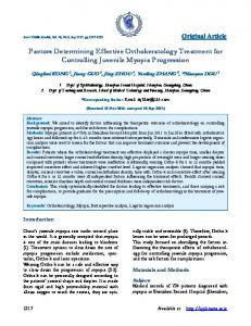
Figure 1: The Z-shaped geometry (top left) is shown under tensile loading (1 % vertical strain). Top middle: No displacement boundary conditions are enforced on the side faces. Top right: We impose periodic boundary conditions on the side faces and affine-periodic boundary conditions at top and bottom. Color (same color scale for all plots) encodes the von Mises stress at the surface of the structure. Bottom: A bigger part of the periodic domain under tensile loading. billion Euro in 2050 [32]. These numbers triggered the development of new treatment techniques such as vertebroplasty and kyphoplasty [19, 16, 34] for vertebral fractures or special implant types for osteoporotic and normal trabecular bone [18, 12]. Finite Element (FE) simulations are used in the development and assessment of those treatment techniques [45, 41, 14, 13, 44]. FE models of whole bones which resolve even the microstructure of trabecular bone require a huge amount of resources [47] and are thus inefficient for parameter studies on the bone-treatment complexes. Instead, continuum models can be used which rely on a proper assessment of the effective material parameters of the bone. These parameters however are almost impossible to be found experimentally, since it is hardly possible to reproduce the in-situ situation of bone specimens. Therefore, they lead just to apparent material properties. Instead, small bone samples of validated rather large scale Micro-FE (µFE) models can be used to determine effective material properties [15]. The in-situ situation of the bone samples is then reproduced numerically. For that, a proper numerical homogenization tool is required. This tool should integrate the true underlying periodic microstructure and incorporate proper boundary conditions. 1.1 Composite Finite Element Simulations Composite Finite Elements (CFE), introduced in [24, 25] and implemented for complicated 3D geometries [35, 42], are an efficient tool to compute elastic deformations of specimens of complicated shape. They have been applied to artificial trabecular objects under uniaxial loading in a parameter study to measure the influence of thinning and degradation of trabeculae on compressive and shearing stiffness [52]. 2


Ω ω

ωM ΩM

Figure 2: For one periodic cell ω in a periodic domain Ω with a complicated microstructure ΩM visible at high resolution, homogenization is the problem of finding an effective material parameter on Ω. Modeling physical experiments on individual small specimens, however, does not yield an appropriate approximation of the effective material properties on the macroscale. E.g. natural boundary conditions on the side faces (if displacement boundary conditions are applied to the top and bottom) permits the specimen to bulge and deform in a way that is not admissible if the specimen is a period cell in a larger scale elastic structure, see Figure 1. 1.2 Homogenization Determining effective material properties for a microscopically inhomogeneous but macroscopically (in general at least statistically) homogeneous material is generally referred to as ‘upscaling’ [4, 49] or ‘homogenization’ [46] and for instance may be used for two-scale FE simulations [2, 3]. It is possible to use multigrid coarsening for upscaling [39, 36], however, using standard geometric coarsening just yields the arithmetic average of the coefficients [38] ignoring any underlying geometric structure. So usually more elaborate coarsening techniques are used [17]. This ‘blackbox’ multigrid method has some automatic way of choosing a coarsening scheme adapted to the problem (in that application: preserving flux across internal interface). Note that this is not algebraic multigrid but respects a grid. We furthermore refer to [5, 6, 10] for overviews on multigrid and other upscaling techniques. Here, we consider a combination of composite finite elements for the numerical solution of the microscopic problem and multigrid methods to assemble macroscopic information for the identification of macroscopic stress and resulting elasticity tensors. Thus, we consider a ‘cell problem’ as discussed e.g. in [1, Chapter 1]. See [46] for some review and theoretical background by Luc Tartar, who introduced the underlying concept in the 1970s. Here, the idea is that macroscopic stresses and strains can be obtained by the simulation of uniaxial loading on a periodic cell with affine-periodic boundary conditions on the microscale. Finally, the homogenized elasticity tensor can be determined from a set of such macroscopic stress-strain pairs. Determining effective elastic properties of cellular solids from unit cells has been of interest for many years [21, 51, 22]. This technique has also been presented in the biomechanics literature [30, 29, 54, 54, 33]. There, periodic cells are frequently denoted as ‘representative volume elements’ [31] or ‘representative elementary volume’ [23].

3


2 Homogenization 2.1 Notation Let us first consider a (geometrically) periodic domain Ω ⊂ R3 with periodic cells ω. Let ΩM ⊂ Ω be the domain of a ω-periodic elastic (micro)structure as shown in Figure 2. Domain Description by Levelset Functions. We assume ΩM (ω-periodic) to be defined by a levelset function [40], that is a function Φ : ω → R (ω-periodic) satisfying {x ∈ ω | Φ(x) < 0 } = ωM

(1)

For instance, this could be obtained from a CT or MRT scan with (denoised) grey values g(x) by Φ(x) = − (g(x) − threshold) or as the signed distance function to some artificial, analytically given object. Periodic Functions. Let a be an ω-periodic coefficient function a : ω → Rd where d is the dimension of the image space of u (e.g. for the scalar test problem d = 1 and can be viewed as a temperature, and for the three-dimensional elasticity problem d = 3). We assume that any ω-periodic function a is smooth on the whole macroscopic domain Ω. We use lowercase letters (u) for analytic quantities (scalar and vector-valued), upper case letters ~ for vectors of discrete values and boldface (U) for discrete quantities and matrices, vector arrows (U) uppercase letters (E) for (block-)matrices and discrete value vectors in the vector-valued problems. Bars will denote the nonoscillatory part u¯ : Ω → Rd , see Section 2.3, whereas tildes will denote the oscillatory periodic part u˜ : ω → Rd of u. A homogenized coefficient a is denoted by a¯ω ≡ const on ω. Discrete ω-periodic quantities are denoted by U # . 2.2 Model Problems Scalar Problem: Steady State of Heat Conduction. described by the partial differential equation (PDE) − div (a(x)∇u(x)) = f (x)

The steady state of heat conduction is in ΩM

(2)

with a : ΩM → R3×3 being an ω-periodic (and possibly anisotropic) diffusion tensor and f : ΩM → R R being an ω-periodic source term with zero average ωM f = 0 (this constraint ensures that a physical steady state is reached). Vector-Valued Problem: Elasticity. Linear elasticity is described by the system of PDEs − div (a(x) ε [u(x)]) = f (x)

in ΩM

(3)

with ε [u] =

1 ∇u + (∇u)T 2

(4)

being the strain tensor for a displacement u, a(x) ≡ a ∈ R3×3×3×3 being the ω-periodic fourth-order elasticity tensor ai jkl = λ δi j δkl + µ δik δ jl + δil δ jk (5) 4


with the Lamé-Navier constants λ and µ that can be computed from Young’s modulus E and Poisson’s ratio ν via E E ·ν , µ= (6) λ= (1 + ν)(1 − 2ν) 2(1 + ν) and with f : ΩM → R3 being an ω-periodic source term (volume force) with zero average ωM f = 0 (else a macroscopic net force would be applied, which contradicts a physical steady state). In our later applications, we only consider the case f ≡ 0, but we will include volume forces in the homogenization for the sake of completeness. R

2.3 Determining Effective Parameters Heat Conduction. In order to obtain an effective diffusion tensor a¯ω , let us consider the heat flux q = a∇u for a given temperature profile u on ω. q is macroscopically given as q¯ω = a¯ω ∇u.

(7)

We want to solve (7) for the matrix a¯ω , so we need at least 3 pairs (ui , q¯ω i )i=0,1,2 with linearly independent ∇ui . For this purpose, consider u¯ with ∇u¯ = ei , where ei is the ith canonical basis vector of R3 , i.e. the temperature u¯ has constant unit gradient. The cell problem is now to find a correction profile u˜ such that the sum u = u¯ + u˜

(8)

is the actual physical temperature profile on the microstructure ΩM having the same macroscopic temperature gradient as u. ¯ From u, we can then compute the heat flux as q¯ω =

Z

Z

Z

q(x) = ωM

a(x)∇u(x) = ωM

a(x)∇ (u¯ + u) ˜ .

(9)

ωM

For each i ∈ {0, 1, 2}, we consider u¯i satisfying ∇u¯i ≡ ei , compute the corresponding u˜i via (14) ω ω and q¯ω i via (9). Plugging q¯i and u¯i into (7) immediately gives us the ith column of a¯ . Elasticity. For obtaining an effective elasticity tensor a¯ω on ω, we consider the (second-order) stress tensor σ = aε [u] for a given deformation profile u on ΩM . σ is macroscopically given as σ¯ ω = a¯ω ε [u] .

(10)

In order to solve Equation (10) for the fourth-order tensor a¯ω , we need 3 × 3 pairs (ui j , σ¯ iωj )i, j=0,1,2 with linearly independent ∇ui . For this purpose, consider u¯ with ∇u¯ = ei ⊗ e j , i.e. u¯ being a ‘unit strain’. The cell problem is now to find a correction profile u˜ such that the sum u = u¯ + u˜

(11)

is the actual physical displacement profile leading to the same macroscopic strain and stress as u. ¯ From the actual displacements u, we can then compute the stress as σ¯ ω =

Z

Z

σ (x) = ωM

Z

a(x)ε [u(x)] = ωM

a(x)ε [u¯ + u] ˜.

(12)

ωM

So in order to obtain a¯ω , we consider u¯i j satisfying ∇u¯ ≡ ei ⊗ e j , compute the corresponding u˜i j via (18) and σ¯ iωj via (12). Plugging all u¯i j and σ¯ iωj (i, j = 0, 1, 2) into (10) allows us to compute a¯ω . Note that the ε [u] ¯ are not linearly independent due to the symmetry of the strain tensor. However, the same symmetry holds in the stress tensor, so effectively Equation (10) is a system of 6 equations in 6 unknowns. 5


2.4 Cell Problems Now, let us describe how to determine the correction terms u˜ described in Section 2.3. Heat Conduction. Plugging the decomposition (8) into the PDE describing the steady state of heat conduction, Equation (2), using linearity and separating unknown and given terms on the left and right hand side, respectively, we obtain: − div (a∇ (u˜ + u)) ¯ =f ⇒ − div (a∇u) ˜ = f + div (a∇u) ¯

in ωM in ωM

(13) (14)

where, as mentioned above, u˜ is ω-periodic. To make the decomposition (8) unique (it is only unique up to addition of a constant), we moreover require u˜ to have zero average: u˜ periodic on ωM

(15)

u˜ = 0

(16)

Z ωM

Elasticity. Plugging the decomposition (11) into the elasticity PDE (3), using linearity and separating unknown and given terms on the left and right hand side, respectively, we obtain: − div (aε [u˜ + u]) ¯ =f ⇒ − div (aε [u]) ˜ = f + div (aε [u]) ¯

in ωM in ωM

(17) (18)

where, again, u˜ is ω-periodic. Note that in the elasticity case, the decomposition (11) in macroscopic and oscillatory part is also not unique: ε [u] = 0 for any u of the form u(x) = Sx + b with b ∈ R3 any vector (translation) and S ∈ R3 any skew-symmetric matrix. So the solution of (18) is unique only up to addition of such an affine displacement. But if we require u˜ periodic on ωM

and

(19)

Z

u˜ = 0,

(20)

ωM

(19) determines the skew-symmetric part and (20) determines the constant part. This is the linearization of the fact that rigid body motions of elastic bodies are force-free, periodic boundary conditions prevent rotations and fixing the average prevents translations. 3 Discretization 3.1 Composite Finite Elements CFE for complicated geometries in 3D [35] are based on the idea that the shape of the microstructure can be represented in the shape of the FE basis functions on a regular grid (rather than in an irregular grid with simple basis functions). They are obtained from standard affine FE on a tetrahedral grid by multiplying the standard basis functions with the characteristic function of the microstructure. The tetrahedral grid results for a subdivision of every cube of a regular cubic grid representing the voxel grid of our image dataset into 6 tetrahedra. Thus, we inherit the uniform structure of the regular cubic grid and its canonical coarse scales, which permits efficient data storage and use of a multigrid solver. For details on this approach and its implementation, we refer to [35, 42]. 6


Let ϕi denote the CFE basis functions for grid nodes xi used to discretize u: U(x) = ∑ ϕi (x)u(xi )

(21)

i

~ = (u(xi ))i be the vector of pointwise values. and let U Then the discrete weak form of the heat conduction PDE (14) with a ≡ 1 is given by Z

⇔

Z ωM

⇔∑

ωM

|

ωM j

j

Z

j

Z

∇U˜ · ∇ϕi = Fϕi − ∇U¯ · ∇ϕi ωM ωM ! Z ~e ∇ ∑ U j ϕ j · ∇ϕi = ∑ ϕ j ~Fj ϕi − ∇ ∇ϕi · ∇ϕ j {z }

~e = U j ∑

=:Li j

Z

ϕi ϕ j {z }

ωM

j

|

∀ϕi

(22)

∀ϕi

(23)

∀ϕi

(24)

!

∑ U~¯ j ϕ j

· ∇ϕi

j

~Fj − ∑ j

Z

~¯ ∇ϕi · ∇ϕ j U j

ωM

=:Mi j

Let us pick up the usual notation M = (Mi j )i j , L = (Li j )i j for the finite element mass and stiffness matrix, respectively. Here the indices i and j are running over all nodal indices for which the support of the classical hat-type basis function intersects the elastic domain ΩM . Then the system above reads: ~e ~ ~¯ LU = B := M ~F − LU

(25)

Now let ψi be the set of vector-valued CFE basis functions. Then the discrete weak form of the elasticity problem (18) with Lamé-Navier elasticity tensor as in (5) is given by Z

Z ˜ ˜ ¯ ¯ : ε [ψi ]) ∀ψi λ divUdivψi + 2µε U : ε [ψi ] = Fψi − (λ divUdivψ i + 2µε [U] ωM ωM Z Z ~ ¯j ˜ ⇔∑ λ divψ j divψi + 2µε ψ j : ε [ψi ] U j = ∑ (26) ψ j ψi ~F j − ∑ Ei j~U ω ω M M j | j j {z } {z } | =:Ei j

=:Mi j

so that the system above reads ~e ~ ¯ EU = B := M~F − E~U.

(27)

If the ψi are ordered in blocks of fixed associated coordinate direction, the matrix E has the 3 × 3 block structure   E00 E01 E02 E = E10 E11 E12  (28) E20 E21 E22

In this section, we explain how periodic boundary conditions can effectively be used in the framework of composite finite elements.

7


Figure 3: 2D periodic boundary conditions. Left: Inactive nodes (right/top boundary) are shown in green, one pair of inactive node and its active counterpart are represented by and symbols, respectively. Right: Supports of basis functions associated to a DOFs in the periodic context. 3.2 Periodic Boundary Conditions Periodic boundary conditions in the context of finite elements are treated by identifying certain degrees of freedom. A node is called inactive if, by periodicity assumption, the value of u at that node is the value of u at the counterpart node and thus no DOF is associated to that node. The node to which we actually associate a DOF and that DOF will be called active counterpart node and active counterpart DOF, respectively. For an active node, the term ‘counterpart’ just refers to the node itself. See Figure 3 for an example. Furthermore, identifying inactive DOFs and their active counterparts means identifying the associated CFE basis functions. This implies that the support of basis functions for such nodes is disconnected within the periodic cell ω, see Figure 3. When working with CFEs on complicated domains, counterparts of inactive nodes are not necessarily degrees of freedom of the CFE grid of the periodic cell ω, even though periodicity implies the same intersection of the domain with periodic faces of ω, see Figure 4 for an example. This is not surprising, however, because a CFE grid for the periodic extension of such domains does have DOFs at such positions. In summary, we observe that the sets of CFE DOFs and their active counterpart DOFs may be distinct and none is subset of the other, see Figure 5 for an example. 3.3 Periodicity Periodicity in data vectors and for matrices must be taken into account when passing between the interpretation of ω as a single cell and a periodic cell, respectively. For simplicity (and computational efficiency, at the cost of additional memory requirement), we use data structures for a full discretization of the periodic cell ω. When dealing with vectors containing point values, the point value at an inactive node is the same as at its active counterpart node, so the corresponding entries in the vector are simply set to zero. We call this operation (periodic) restriction and denote it by the symbol Pv . The inverse Pv−1 , filling those entries back in by copying them, will be referred to as (periodic) extension. The identification of basis functions leads to a larger support for certain basis functions. When dealing with integrated quantities in a data vector or when dealing with matrices (containing integrals of basis functions or their derivatives), this translates to adding entries of inactive nodes to the entries of their active counterparts. Let us call this operation (periodic) collapsing and denote it by Pb . We use the notation X # for periodized objects (matrices, vectors).

8


Figure 4: The CFE grid for one periodic cell does not have a DOF at the bottom left node () even though that node is the counterpart node of the two nodes. The thick red line indicates the level set boundary of the periodic cell ωM . 3.4 Dealing with the constraints in the discrete case The constraint

R

Z

Z

U = 0 for a discrete function U can be rewritten as follows:

U= ωM

ωM

U1 = R

1

Z

ωM 1 ωM

1U = 0 ⇔

1 ~ =0 M~1 · U M~1 ·~1

(29)

~ the nodal vector corresponding to u. To where M is the FE mass matrix, ~1 is the all-1 vector and U simplify notation, let us define J~ :=

1 M~1. M~1 ·~1

(30)

In the heat conduction case, the resulting system of equations is given by (discretizing (14) and (15)) ~e # ~ # L#U =B

(31)

~e ~¯ where L# = Pb (L) and B# = Pb (M F) − Pb (LU). The system matrix has a one-dimensional eigenspace corresponding to one additive constant. It becomes uniquely solvable if we require the additional equation #

~e = 0 J~# · U where J~# =

M #~1# M #~1# ·~1#

(32) with M # = Pb (M) and ~1# := Pv (~1). R

Now, let us consider how to project onto the subspace of given constraints. Let s := {u| u = 0} be the subspace of all temperature profiles satisfying the average-zero constraint. The projection R onto s is given by Πs u = u − ( u) 1 for any temperature profile u. In discrete form, projection onto ~ ⊥ using J~ defined in (30) is the subspace S := span(J) ~ =U ~ − J~ · U ~ ~1. ΠSU (33) In the vector-valued case, the system of equations (cf. (31)) is  #  #   # ~e # # ~B E00 E01 E02 U 0  0 # # ~  E # E # E #   ~ = B   e U 1 10 11 12 1  # # # # ~ # E20 E21 E22 B ~e 2 U 2 9

(34)


Figure 5: The CFE grid for one periodic cell has the set of DOFs on the left, active counterpart nodes are those on the right. These sets are mutually not contained. ~e ¯ The constraint (32) is now ‘zero with E# = Pb (E), right hand side ~B# = Pb (MF) − Pb (E~U). average displacement in all three space directions’: ~e # ~# ~e # ~# ~e # J~# · U 0 = J · U 1 = J · U 2 = 0,

(35)

so projection (33) is now performed in the three components separately. 3.5 Numerical Algorithms for the Cell Problem Heat Conduction. tion term:

Let us now summarize the steps necessary for computing one periodic correc-

~¯ ~F, e ~1 and matrices M, L 1. set up vectors U, 2. compute right hand side 3. periodize M, L,~1

~¯ ~# := P (M~F) e − Pb (LU) B b

M # := Pb (M) L# := Pb (L) ~1# := Pv (~1)

4. compute constraint vector

J~# =

M #~1# M #~1# ·~1#

5. solve the system ~e # ~# ~e # ~¯ # L#U = B = (M F) − (LU) ~e # subject to J~# · U =0 6. periodically extend and add macroscopic part

~e # ~¯ ~ = Pv−1 (U U ) +U

Elasticity. In the vector-valued case, we have a 3 × 3 block system of equations instead of the matrix L on the left hand side, subject to constraints for all three components of the displacement. Other than that, the procedure is the same. 4 Projecting Solvers In this section, we describe appropriate iterative solvers for the constrained linear system problem to be solved for the periodic cell problem (cf. item 5 in the procedure in Section 3.5). 10


4.1 Projecting Conjugate Gradient Solver [42] shows that a conjugate gradient solver [28] may encounter difficulties for systems of equations resulting from CFE discretizations because small virtual CFE tetrahedra may lead to large condition numbers. In many situations this can be remedied by (block-)diagonal preconditioning [43]. However, we only use CG as the solver on the coarsest grid and do not encounter this problem. CG, being a Krylov-space method [7], has the nice property that (in exact arithmetics) the iterates ~ stay in the subspace satisfying our J-constraints for uniqueness if the starting value lies inside it. As we usually start with the zero initial guess, this condition is trivially satisfied. Due to finite precision in the implementation, however, we still need to check whether the ~ J-constraints are satisfied after each CG update. If necessary (e.g. constraint violated by more than a given threshold), the iterate needs to be projected back to the space S as shown in (33) to avoid ‘drifting’ of the numerical solution. 4.2 Projecting Multigrid Solver Periodicity changes neighborhood relations, this means that any inactive node p being identified with its active counterpart node f makes p’s neighbors f ’s neighbors and vice versa, see Figure 6. A multigrid algorithm for the composite finite elements is straightforward. Let us suppose that the underlying hexahedral grid is dyadic and generated by successive splitting of edges leading to an octree structure with underlying hierarchy of tetrahedral grids. We define the coarse grid basis functions and the prolongation and restriction operators respectively by local Galerkin products [26] on regular tetrahedral meshes. This involves the weights 1, 1/2, and 0 in the prolongation matrices for the interpolation from a coarse grid-level to the next finer grid-level. The restriction is, as usual, the transpose of the prolongation. Coarse grid basis functions are obtained as the corresponding weighted sums of the fine grid basis functions. This standard approach leads to piecewise affine basis functions on the coarse tetrahedral grids which are cut off by multiplication with a characteristic function of the computational elastic domain ΩM . Note that in general the coarse grids are not able to resolve the computational domain. Consequently, the support of a coarse grid basis function may consist of several disconnected components. However, it is easy to see that the basis functions still form a partition of unity on the computational domain. Finally, by standard Galerkin coarsening, one defines corresponding coarse grid linear systems. We then use a multigrid method with symmetric Gauß-Seidel iterations [26] as a smoother. For scalar problems, the Gauß-Seidel smoother is a standard one, for vector valued problems, we use a Block-Gauß-Seidel method. The unknowns are (implicitly reordered and) indexed in such a way that we treat the spatial components of our solution simultaneously. In case of a three-dimensional problem, we use Gauß-Seidel iterations on 3 × 3 blocks. In our computations in Section 6, V-cycles with no more than 3 pre- and post-smoothing steps turned out to be a reasonable choice. We now explain the modifications to the CFE multigrid solver presented in [35, 42] that are necessary for our purposes here. For an introduction to multigrid methods (originally introduced in [8]), we refer to [26, 9]. Prolongation and Restriction in the Periodic Case. The prolongation operator must respect the additional neighborhood relations introduced by periodicity and the fact that they are dealing with integrated quantities, which have to be collapsed periodically. As usual, the prolongation weight from a coarse grid node c to a fine grid node f is simply the value of the coarse grid basis function located at c evaluated at f . In our case these weights are 0, 0.5, or 1. This means that we loop over all coarse nodes which are active DOF nodes or whose active counterpart nodes are active DOF 11


Figure 6: Identification (red arrows) of an inactive node with its active counterpart changes standard neighborhoods for prolongation and restriction. Left: All fine (blue) grid nodes ♦ are active neighbors of coarse (black) grid node . Right: At a corner, we have multiple inactive counterparts and their active neighbors ♦ as fine grid neighbors of the active coarse grid node . nodes. In either case, we prolongate only to a fine neighbor of the coarse node if the fine node is an active DOF node, see Figure 6. As in the non-periodic case, the restriction is the adjoint (transpose) of the prolongation and subject to the same modifications due to periodicity. Coarsening of the operators is computed as above by precomposing with prolongation and postcomposing with restriction. This can be implemented by explicit multiplication of sparse matrices or, as the neighborhood structure of grid points and thus the sparsity structure of the matrices is known a priori, by direct computation of the coarse matrix. Gauß-Seidel Smoothing. As a smoothing operation, we use standard or block-wise Gauß-Seidel smoothing [26] on the set of unknowns after periodization. No further modification of the smoothing is necessary. Constraints and Projection. Coarsened J~ constraints, see Equation (30), are computed using all-1 vectors corresponding to the coarse grid and using coarsened mass matrices. For this purpose, we use the same coarsening method as for the system matrices (in the scalar case). The smoothing operations used in our multigrid solver do not guarantee that we stay inside the subspace satisfying the J~ constraints, so the multigrid solver has to perform projections to the space S as shown in (33). Our approach is to perform this projection after presmoothing, coarse-grid correction and postsmoothing on each but the coarsest level. On the coarsest level, we use a projecting CG solver to make the coarsest problem uniquely solvable. The coarsening process accumulates rounding errors in the coarsened system matrices so that constant vectors no longer exactly lie in the zero eigenspace. Thus, the projection may destroy convergence of the CG solver. To remedy this, observe that constant vectors are eigenvectors to the eigenvalue 0 if and only if each row of the matrix has sum zero. If this condition is not satisfied due to rounding errors, we can enforce it by modifying the diagonal entry in such rows. This modification is of the same magnitude as the rounding errors.

12


R ∈ SO(3)

Figure 7: Orthotropy axes in the actual configuration (right) are not aligned with the coordinate axes but rotated from a reference configuration (left) by some rotation R. 5 Orthotropy Directions In this section, we present a method how to determine whether a given macroscopic elasticity tensor describes orthotropic material properties. Hence, we have to identify orthotropy axes are not aligned with the coordinate axes. A straightforward idea, see e.g. [48, 53], is to determine the rotation R ∈ SO(3) that ‘best rotates the effective tensor to an orthotropic one’. Such a method immediately provides a mechanism to check whether the orthotropy assumption was justified: for the optimal rotation the remaining defect from an orthotropic structure of the elasticity tensor is a measure for the lack of orthotropy. Rotations in R ∈ SO(3) can be described as R = R(α, β , γ) = Rxy (α)Rxz (β )Ryz (γ)     cos α − sin α 0 cos β 0 − sin β 1 0 0 1 0  0 cos γ − sin γ  =  sin α cos α 0  0 0 0 1 sin β 0 cos β 0 sin γ cos γ

(36) (37)

with α, β , γ ∈ A := (−π, π] being the rotations in the xy, xz and yz plane, respectively. Note that rotations do not commute, the inverse rotation is given by Rback (α, β , γ) = Ryz (−γ)Rxz (−β )Rxy (−α)

(38)

5.1 Rotation of Tensors Heat Conduction. Suppose we have a material with orthotropic heat conductivity a for which the orthotropy axes are not aligned with the coordinate axes but rotated by some rotation matrix R ∈ SO(3), see Figure 7. Let u denote our temperature in the actual configuration, obtained from a profile u? in the aligned reference configuration. Then x? = RT x ,

u(x) = u? (x? )

∇u(x) = R∇u? (x? ) ,

(39)

if gradients are written as column vectors. Moreover, q? = a? ∇u? = a? RT ∇u

⇒

q = Rq? = Ra? RT ∇u

⇒ a = Ra? RT

(40) (41)

or, written in components and using the Einstein summation convention we obtain amn = Rmi a?i j RTjn = Rmi Rn j a?i j , which describes how the conductivity tensor changes under rotation.

13


Elasticity. In the vector-valued case, also our function u must be rotated and its component-wise gradients are interpreted as rows of ∇u, hence we obtain u(x) = Ru? (x? ) , ∇u(x) = R∇u? (x? )RT T 1 1 ⇒ ε [u] = ∇u? + ∇u?T = R∇u? (x? )RT + R∇u? (x? )RT 2 2 1 = R∇u? (x? )RT + RT T ∇u? (x? )RT = Rε [u? ] RT 2

(42) (43) (44)

Moreover, from σ ? = a? ε [u? ] = a? RT ε [u] R we deduce σ = Rσ ? RT = R a? RT ε [u] R RT . Again written in components, we finally get ? T σmn = Rmi ai jkl Rl p ε [u] po Rok RTjn = Rmi Rn j Rok R pl a?i jkl ε [u]op (45) | {z } =ε[u]op

⇒ amnop = Rmi Rn j Rok R pl a?i jkl ,

(46)

which describes the effect of a given rotation on the elasticity tensor. 5.2 Finding the Rotation in the Elasticity Case Voigt’s notation. Due to symmetry of strains and stresses, the 3 × 3 strain and stress tensors can be written as vectors of length 6 and the 3 × 3 × 3 × 3 fourth order elasticity tensor can be written as a symmetric 6 × 6 matrix, called Voigt’s notation [50]:      σxx a00 a01 a02 a03 a04 a05 εxx σyy  a10 a11 a12 a13 a14 a15   εyy        σzz  a20 a21 a22 a23 a24 a25   εzz   =   (47) σyz  a30 a31 a32 a33 a34 a35  2εyz       σxz  a40 a41 a42 a43 a44 a45  2εxz  σxy a50 a51 a52 a53 a54 a55 2εxy We will switch between standard tensor notation (with four indices) and Voigt’s notation (with two indices). Orthotropic Materials. For an orthotropic material whose orthotropy axes coincide with the coordinate axes, the upper right 3 × 3 (and, due to symmetry, also the lower left 3 × 3) block of a is zero and the lower right 3 × 3 block is diagonal. Now, we consider the following minimization problem to determine a measure for the orthotropy using a method similar to the one presented in [48]. Let F : R3×3×3×3 → R+ be some function penalizing deviations of E from an aligned orthotropic tensor (see below). Then minimize Ga (α, β , γ) = F Rmi Rn j Rok R pl ai jkl (48) over the admissible set A where R is the matrix Rback (α, β , γ). As F, we choose a function similar to [48] but incorporate a weighting which reflects that entries in the Voigt tensor represent up to four entries of the full fourth order tensor. Let F(a) =

2 ∑2i=0 ∑5j=3 a2i j + 2 ∑5i=3 ∑2j=0 a2i j + 4 ∑5i, j=3,i6= j a2i j 1 ∑2i, j=0 a2i j + 4 ∑5i= j=3 a2i j 14

(49)


y x z

Figure 8: Sample geometry: d/l = (0.4, 0.3, 0.2) and corresponding macroscopic, orthotropic elasticity tensor visualized. be the sum of the squared undesired tensor entries divided by the sum of squares of the desired entries. For an aligned orthotropic tensor a, we obviously have F(a) = 0. An intrinsic difficulty in this optimization is that the function G is not convex. However, G is not highly oscillatory and a function of only three variables, so there is no need to put much effort in finding an efficient minimization method. Our approach is to simply discretize A with a certain angular resolution, find the discrete minimum and continue choosing a smaller interval near the discrete minimum until a fixed accuracy in the angles is reached. Compared to the actual finite element simulations (nine per specimen), the workload of this postprocessing is negligible. 6 Results We will now consider different geometric objects for which we determine effective elasticity parameters by our homogenization method. To emphasize that we are considering artificial objects, we assume an edge length of 1 m, microscopic isotropy with a Young’s modulus of E = 1 Pa. Moreover, we set Poisson’s ratio ν = 0.33, resulting in λ = 0.747 and µ = 0.376. 6.1 Visualization We visualize the macroscopic elasticity tensors obtained from our simulations by deformed and colored spheres, as suggested by [11, 27]. For this purpose, let n be any unit vector in R3 (corresponding to a point on the unit sphere). Then compute the compressive stiffness in direction n we compute step by step N = n ⊗ n (Ni j = ni n j ), S = EN (Si j = Ei jkl Nkl ) and finally σ = N : S (σ = Ni j Si j ) and draw the shape {σ n|knk = 1}. Moreover we compute the bulk modulus, i.e. the resistance of the material against a volumetric deformation, trS = ∑i Sii and color code the deformed sphere with the resulting value (hsv blue to red, blue corresponds to zero, red to maximal value). 6.2 Aligned Orthotropic Specimens As a first example, let us consider an object as in Figure 8: 1 × 1 × 1 cylinders of distanceto-length ratios d/l = (0.4, 0.3, 0.2). Using different computational resolutions, we obtain the following rotations for the best orthotropic description as described in Section 5.2 and the following macroscopic elasticity tensors in Pa:

15


93 : rotation (−8.50 · 10−2 , −4.52 · 10−2 , −2.23 · 10−2 )◦ ,        

0.126657 0.012256 0.003419 0.012355 0.079110 0.002030 0.003537 0.002092 0.022781 −1.64 · 10−4 −4.53 · 10−5 −1.90 · 10−4 −3.83 · 10−6 8.54 · 10−5 −1.06 · 10−4 −1.84 · 10−4 −3.74 · 10−4 1.88 · 10−4

−1.73 · 10−4 6.88 · 10−7 −2.37 · 10−4 −5.08 · 10−5 9.45 · 10−5 −5.02 · 10−4 −1.93 · 10−4 −8.81 · 10−5 1.16 · 10−4 0.002714 −3.76 · 10−4 −1.21 · 10−4 −4.02 · 10−4 0.003323 1.31 · 10−4 −1.22 · 10−4 1.35 · 10−4 0.010845

       

333 : rotation (−1.17 · 10−2 , −1.98 · 10−2 , 1.50 · 10−2 )◦ , 

0.128019 0.011907 0.005881  0.012029 0.076170 0.003064   0.005877 0.003137 0.039644   −2.64 · 10−5 −4.60 · 10−5 −6.70 · 10−5   −9.23 · 10−6 3.34 · 10−5 −2.40 · 10−5 −1.47 · 10−5 −1.19 · 10−5 5.47 · 10−5

−2.70 · 10−5 −4.83 · 10−6 −1.25 · 10−5 −1.76 · 10−5 4.00 · 10−5 −4.51 · 10−5 −6.04 · 10−5 −2.65 · 10−5 1.49 · 10−5 0.001768 −7.86 · 10−5 −1.86 · 10−5 −7.33 · 10−5 0.002691 2.81 · 10−5 −2.34 · 10−5 3.37 · 10−5 0.007038

       

1293 : rotation (−1.22 · 10−3 , −2.50 · 10−3 , 1.34 · 10−3 )◦ ,        

0.132389 0.012208 0.005717 0.012258 0.081428 0.003551 0.005751 0.003553 0.039215 −3.28 · 10−6 −4.75 · 10−6 −1.10 · 10−5 −1.10 · 10−6 4.23 · 10−6 −3.77 · 10−6 −6 −6.48 · 10 −1.14 · 10−5 5.44 · 10−6

−3.58 · 10−6 −1.09 · 10−6 −6.50 · 10−6 −4.78 · 10−6 3.98 · 10−6 −1.34 · 10−5 −1.04 · 10−5 −4.29 · 10−6 2.94 · 10−6 0.001733 −8.19 · 10−6 −1.72 · 10−6 −8.81 · 10−6 0.002222 3.50 · 10−6 −6 −6 −2.00 · 10 3.56 · 10 0.006709

       

2573 : rotation (−4.65 · 10−4 , −8.84 · 10−4 , 2.79 · 10−4 )◦ , 

0.132314 0.012126 0.005700  0.012143 0.081494 0.003596   0.005700 0.003588 0.039394   −1.38 · 10−6 −1.85 · 10−6 −4.29 · 10−6   −4.10 · 10−7 1.40 · 10−6 −1.37 · 10−6 −3.71 · 10−6 −6.58 · 10−6 2.62 · 10−6

−1.65 · 10−6 −3.92 · 10−7 −3.64 · 10−6 −1.94 · 10−6 1.33 · 10−6 −7.35 · 10−6 −4.32 · 10−6 −1.54 · 10−6 1.43 · 10−6 0.001718 −2.83 · 10−6 −5.03 · 10−7 −3.01 · 10−6 0.002182 1.26 · 10−6 −5.68 · 10−7 1.25 · 10−6 0.006620

       

Hence, we experimentally observe convergence for increasing resolution of the cell geometry. In the tensor listing above, all entries that should be zero for an orthotropic material are shown in exponential notation whereas the nonzero entries are printed in decimal notation. We observe the following: • With increasing resolution, the rotation angles (that should be exactly zero for our aligned structures) converge to zero. This error may be due to the fact that the decomposition of cubes in six tetrahedra is not symmetric and has preferred directions, so that the discretization of the object has corresponding sub-pixel errors. • Similarly, the tensor entries that are zero for a perfectly aligned orthotropic tensor, converge to zero with increasing computational resolution. For the 93 resolution, entries in the lower right diagonal block are of the same magnitude (10−4 ) as some entries that should be zero; at computational resolution 2573 , the difference is two orders of magnitude. • In the upper left block of the Voigt tensor, we observe convergence to symmetry.

16


z y

x

Figure 9: Sample geometry: 5 by 5 by 5 with d/l = (0.4, 0.3, 0.2). Comparison to Simulations on Individual Specimens. Let us now compare these homogenization results to compressive and shearing stiffness obtained from the simulation on the nonhomogenized microstructure consisting of n × n × n structural elements (see [52]) subject to the following boundary conditions: two opposite faces of the bounding cube are displaced by a fixed value, no boundary conditions are imposed on the side faces. One such structure is shown in Figure 9. For different values of n, we obtain the following stiffnesses for compression in x direction: 1 × 1 × 1 at resolution 1293 : 0.133939 Pa 5 × 5 × 5 at resolution 1293 : 0.133248 Pa 10 × 10 × 10 at resolution 1293 : 0.132871 Pa 15 × 15 × 15 at resolution 2573 : 0.132860 Pa 20 × 20 × 20 at resolution 2573 : 0.132436 Pa Moreover, for 10 × 10 × 10 at resolution 2573 , we perform all uniaxial compression and shear loading cases and obtain: x compression: 0.132726 Pa y compression: 0.082275 Pa z compression: 0.039549 Pa yz shearing: 0.0021291, 0.0020593 Pa xz shearing: 0.0029628, 0.0026015 Pa xy shearing: 0.0072422, 0.0068263 Pa Here, compressive stiffnesses are almost the same as the ones obtained from homogenization, so periodic or Neumann boundary conditions on side faces make almost no difference. This may be due to the fact that the models do not include geometric nonlinearities such as buckling. Thus, certain deformation modi are possibly not reflected by the simulations.

17


z y x

Figure 10: A periodic rotated 5 × 5 × 5 rod sample with constant d/l = (0.4, 0.4, 0.4) and corresponding macroscopic, orthotropic elasticity tensor. 6.3 Non-Aligned Orthotropic Specimens As a non-aligned orthotropic specimen, we use a 5×5×5 structure with the same d/l = (0.4, 0.4, 0.4) in all space directions, scaled and rotated in such a way (around the x axes by arctan 15 ) that we obtain a geometrically periodic specimen, see Figure 10. We obtain the macroscopic elasticity tensor        

0.152681 0.019893 0.020356 −4.31 · 10−5 −5.99 · 10−5 −9.41 · 10−5 0.019934 0.140770 0.027302 −0.017407 7.45 · 10−5 −1.32 · 10−5 0.020442 0.027346 0.141225 0.017398 −4.16 · 10−5 1.15 · 10−4 −4 −4 −1.09 · 10 −0.017421 0.017344 0.022457 −1.67 · 10 −5.65 · 10−5 −5.84 · 10−5 5.87 · 10−5 −5.18 · 10−5 −1.71 · 10−4 0.015305 2.31 · 10−4 −5.98 · 10−5 5.13 · 10−6 1.51 · 10−4 −4.29 · 10−5 2.05 · 10−4 0.014825

       

which clearly does not have aligned orthotropic structure. After a minimization of the function G(·) above we obtain the optimal set of rotations (−11.33, 2.25 · 10−3 , −1.72 · 10−2 )◦ , and the resulting approximately orthotropic tensor        

0.152681 0.019928 0.020322 0.019996 0.148068 0.020053 0.020381 0.020067 0.148455 −1.98 · 10−4 −7.37 · 10−5 −9.41 · 10−5 −7.30 · 10−5 1.23 · 10−4 −8.20 · 10−5 −1.62 · 10−5 −2.65 · 10−5 1.49 · 10−4

−1.29 · 10−4 −8.13 · 10−5 −4.96 · 10−5 −5.38 · 10−5 1.35 · 10−4 −4.27 · 10−5 −3.43 · 10−5 −7.84 · 10−5 1.07 · 10−4 −4 0.015193 −1.45 · 10 −4.94 · 10−5 −1.47 · 10−4 0.015371 1.22 · 10−4 −3.95 · 10−5 9.60 · 10−5 0.014759

       

6.4 Nonorthotrpoic Honeycomb Structure Consider the honeycomb-cylindrical structure shown in Figure 11. Assuming edge length of 1 m, E = 1 Pa and ν = 0.33, we obtain the macroscopic elasticity tensor        

0.162208 0.076465 0.078762 7.50 · 10−12 −1.57 · 10−12 0.002110 0.079205 0.140852 0.072619 −7.84 · 10−12 6.25 · 10−12 0.002309 0.079666 0.071715 0.362591 3.13 · 10−12 3.35 · 10−12 0.001458 4.45 · 10−11 −1.85 · 10−12 1.41 · 10−11 0.066276 0.000599 −7.13 · 10−13 −3.50 · 10−11 4.70 · 10−12 −1.00 · 10−11 0.000563 0.072523 1.64 · 10−11 0.001332 0.001463 0.000922 −2.59 · 10−13 1.33 · 10−12 0.025120

       

for which our optimization yields rotation angles (−4.38 · 10−9 , −4.38 · 10−9 , 2.08)◦ and a rotated tensor        

0.162368 0.076484 0.078821 7.35 · 10−12 −6.00 · 10−12 0.000816 0.079335 0.140544 0.072560 −1.26 · 10−11 6.53 · 10−12 0.002715 0.079762 0.071619 0.362591 −8.51 · 10−12 −7.29 · 10−12 0.001165 4.55 · 10−11 −6.38 · 10−12 2.96 · 10−12 0.066242 0.000371 −6.20 · 10−12 −3.71 · 10−11 3.88 · 10−12 −2.03 · 10−11 0.000335 0.072557 1.41 · 10−11 0.000140 0.001970 0.000696 −4.05 · 10−12 −1.98 · 10−12 0.025193

which still shows the lack of orthotropy. 18

       


y x

z

Figure 11: Nonorthotropic honeycomb-cylindrical structure and corresponding macroscopic elasticity tensor. 7 Conclusions This paper gives an introduction to numerical homogenization in the context of periodic microstructures in linearized elasticity. It is meant as a proof of concept and demonstrates the applicability of multigrid composite finite element methods in the biomechanical upscaling context. A limitation of the homogenization method presented here is that it can only be applied to geometrically periodic specimens. Future work will be devoted to stochastic media and non-cubic, non-periodic samples as they are actually used in many experimental setups for the study of bone microstructures. A further limitation of our applications is the linear elasticity model. 8 Acknowledgments This work was supported by the DFG project RU567/8-2 ‘Multi scale Simulation and Validation of the Elastic Microstructures of Vertebral Bodies’ and the DFG project WI 1352/13-1 ‘Frakturrisiko von Wirbelkörpern unter Berücksichtigung von inhomogenen Dichteverteilungen und lokal unterschiedlichen Trabekelausrichtungen’. The authors would like to thank Sergio Conti and Martin Lenz for their advice on homogenization and Benedikt Wirth for helpful discussions about the rotations in Section 5. Moreover, we would like to thank the Hausdorff Center for Mathematics in Bonn for CPU time on their compute server hydra. References [1] Grégoire Allaire, Shape optimization by the homogenization method, Applied Mathematical Sciences, vol. 146, Springer-Verlag, New York, 2002. [2] Todd Arbogast, Numerical subgrid upscaling of two-phase flow in porous media, TICAM Report 99-30, University of Texas at Austin, August 2000. [3]

, Numerical treatment of multiphase flow in porous media, Lecture Notes in Physics, vol. 552, ch. Numerical Subgrid Upscaling of Two-Phase Flow in Porous Media, pp. 35–49, Springer, 2000.

[4]

, Current trends in scientific computing, Contemporary Mathematics, ch. An overview of subgrid upscaling for elliptic problems in mixed form, pp. 21–32, AMS, 2003.

19


[5] Todd Arbogast, Susan Minkoff, and Phil Keenan, An operator-based approach to upscaling the pressure equation, TICAM Report 97-30, University of Texas at Austin, November 1997. [6] Todd Arbogast, Susan E. Minkoff, and Philip T. Keenan, Computational methods in contamination and remediation of water resources, vol. 1, Computational Methods in Water Resources, no. XII, ch. An operator-based approach to upscaling the pressure equation, pp. 405–412, Computational Mechanics Publications, 1998. [7] Owe Axelsson, Iterative solution methods, Cambridge University Press, 1994. [8] Achi Brandt, Multi-level adaptive solutions to boundary-value problems, Mathematics of Computation 31 (1977), no. 138, 333–390. [9] Achi Brandt and Dorit Ron, Multigrid solvers and multilevel optimization strategies, Combinatorial Optimization, vol. 14, ch. 1, pp. 1–69, Kluwer Academic Publishers, 2002. [10] Achi E. Brandt, Methods of systematic upscaling, Tech. Report MCS06-05, Weizmann Institute of Science, 2006. [11] Antonio Cazzani and Marco Rovati, Extrema of Young’s modulus for cubic and transversely isotropic solids, International Journal of Solids and Structures 40 (2003), 1713–1744. [12] M. C. Chang, C. L. Liu, and T. H. Chen, Polymethylmethacrylate augmentation of pedicle screw for osteoporotic spinal surgery: a novel technique, Spine 33 (2008), E317–E324. [13] Chen-Sheng Chen, Wen-Jer Chen, Cheng-Kung Cheng, Shya-Hua Eric Jao, Shan-Chang Chueh, and Chang-Chih Wang, Failure analysis of broken pedicle screws on spinal instrumentation, Medical Engineering & Physics 25 (2005), no. 6, 487–496. [14] S.-I. Chen, R.-M. Lin, and C.-H. Chang, Biomechanical investigation of pedicle screw–vertebrae complex a finite element approach using bonded and contact interface conditions, Medical Engineering & Physics 25 (2003), 275–282. [15] Y. Chevalier, D. Pahr, H. Allmer, M. Charlebois, and P. Zysset, Validation of a voxel-based FE method for prediction of the uniaxial apparent modulus of human trabecular bone using macroscopic mechanical tests and nanoindentation, Journal of Biomechanics 40 (2007), no. 15, 3333–3340. [16] J. H. Chi and Z. L. Gokaslan, Vertebroplasty and kyphoplasty for spinal metastases, Current Opinion in Supportive and Palliative Care 2 (2008), no. 1, 9–13. [17] Joel E. Dendy Jr., Black box multigrid, Journal of Computational Physics 48 (1982), 366–386. [18] P. Fransen, Increasing pedicle screw anchoring in the osteoporotic spine by cement injection through the implant. Technical note and report of three cases, Journal of Neurosurgery: Spine 7 (2007), no. 3, 366–369. [19] M. J. Gardner, D. Demetrakopoulos, M. K. Shindle, M. H. Griffith, and J. M. Lane, Osteoporosis and skeletal fractures, HSS Journal 2 (2006), no. 1, 62–69. [20] H. K. Genant, M. D. Guglielmi, and M. Jergas (eds.), Bone densitometry and osteoporosis, SpringerVerlag, 1998. [21] L. J. Gibson, The mechanical behaviour of cancellous bone, Journal of Biomechanics 18 (1985), 317–328. [22]

, Biomechanics of cellular solids, Journal of Biomechanics 38 (2005), 377–399.

20


[23] Y. Guéguen, M. Le Ravalec, and L. Ricard, Upscaling: Effective medium theory, numerical methods and the fractal dream, Pure and Applied Geophysics 163 (2006), 1175–1192, DOI:10.1007/s00024006-0053-y. [24] W. Hackbusch and S. Sauter, Composite finite elements for the approximation of PDEs on domains with complicated micro-structures, Numerische Mathematik 75 (1997), 447–472. [25] W. Hackbusch and S. A. Sauter, Composite finite elements for problems containing small geometric details. Part II: Implementation and numerical results, Computing and Visualization in Science 1 (1997), no. 1, 15–25. [26] Wolfgang Hackbusch, Multi-grid methods and applications, Springer Series in Computational Mathematics, vol. 4, Springer, 1985. [27] Q.-C. He and A. Curnier, A more fundamental approach to damaged elastic stress-strain relations, International Journal for Solids and Structures 32 (1995), no. 10, 1433–1457. [28] Magnus R. Hestenes and Eduard Stiefel, Methods of conjugate gradients for solving linear systems, Journal of Research of the National Bureau of Standards 49 (1952), no. 6, 409–436. [29] S. J. Hollister, J. M. Brennan, and N. Kikuchi, A homogenization sampling procedure for calculating trabecular bone effective stiffness and tissue level stresses, Journal of Biomechanics 27 (1994), no. 4, 433–444. [30] S. J. Hollister, D. P. Fyhrie, K. J. Jepsen, and S. A. Goldstein, Application of homogenziaton theory to the study of trabecular bone mechanics, Journal of Biomechanics 24 (1991), no. 9, 825–839. [31] S. J. Hollister and N. Kikuchi, A comparison of homogenization and standard mechanics analyses for periodic porous composites, Computational Mechanics 10 (1992), 73–95. [32] J. A. Kanis and O. Johnell, Requirements for DXA for the management of osteoporosis in Europe, Osteoporosis International 16 (2005), 229–238. [33] P. Kowalczyk, Orthotropic properties of cancellous bone modelled as parameterized cellular material, Computer Methods in Biomechanics and Biomedical Engineering 9 (2006), 135–147. [34] E. Michael Lewiecki, Vertebroplasty and kyphoplasty update, Current osteoporosis reports 6 (2008), no. 3, 114–119. [35] Florian Liehr, Tobias Preusser, Martin Rumpf, Stefan Sauter, and Lars Ole Schwen, Composite finite elements for 3D image based computing, Computing and Visualization in Science 12 (2009), no. 4, 171–188, DOI:10.1007/s00791-008-0093-1. [36] Scott P. MacLachlan and J. David Moulton, Multilevel upscaling through variational coarsening, Water Resources Research 42 (2006), W02418, DOI:10.1029/2005WR003940. [37] L. J. Melton III, M. Thamer, N. F. Ray, J. K. Chan, C. H. Chesnut III, T. A. Einhorn, C. C. Johnston, L. G. Raisz, S. L. Silverman, and E. S. Siris, Fractures attributable to osteoporosis: report from the national osteoporosis foundation, Journal of Bone Mineral Research 12 (1997), 16–23. [38] J. D. Moulton, S. Knapek, and J. E. Dendy, Multilevel upscaling in heterogeneous porous media, CNLS research highlight, Los Alamos National Laboratories, January 1999. [39] J. David Moulton, Joel E. Dendy Jr., and James M. Hyman, The black box multigrid numerical homogenization algorithm, Journal of Computational Physics 142 (1998), 80–108, Article No. CP985911. [40] S. J. Osher and J. A. Sethian, Fronts propagating with curvature dependent speed: Algorithms based on Hamilton–Jacobi formulations, Journal of Computational Physics 79 (1988), 12–49.

21


[41] A. Polikeit, S. J. Ferguson, L. P. Nolte, and T. E. Orr, The importance of the endplates for the interbody cages in the lumbar spine, European Spine Journal 12 (2003), 556–561. [42] Tobias Preusser, Martin Rumpf, and Lars Ole Schwen, Finite element simulation of bone microstructures, Proceedings of the 14th Workshop on the Finite Element Method in Biomedical Engineering, Biomechanics and Related Fields, University of Ulm, July 18-19 2007, pp. 52–66. [43] Alfio Quarteroni, Riccardo Sacco, and Fausto Saleri, Numerical mathematics, Texts in Applied Mathematics, vol. 37, Springer-Verlag, New York, 2000. [44] A. Rohlmann, T. Zander, and G. Bergmann, Spinal loads after osteoporotic vertebral fractures treated by vertebroplasty or kyphoplasty, European Spine Journal 15 (2006), 1255–1264. [45] A. Rohlmann, T. Zander, M. Fehrmann, C. Klöckner, and G. Bergmann, Einfluss eines doppelten Zwischenwirbelkäfigs auf das mechanische Verhalten der Lendenwirbelsäule, Biomedizinische Technik 47 (2002), 124–129. [46] Luc Tartar, Optimal shape design, Lecture Notes in Mathematics, vol. 1740, ch. An Introduction to the Homogenization Method in Optimal Design, pp. 47–156, Springer, 2001. [47] B. van Rietbergen, R. Müller, D. Ulrich, P. Rüegsegger, and R. Huiskes, Tissue stresses and strain in trabeculae of a canine proximal femur can be quantified from computer reconstructions, Journal of Biomechanics 32 (1999), no. 2, 165–173. [48] B. van Rietbergen, A. Odgaard, J. Kabel, and R. Huiskes, Direct mechanics assessment of elastic symmetries and properties of trabecular bone architecture, Journal of Biomechanics 29 (1996), no. 12, 1653–1657, Technical Note. [49] Tetyana Vdovina, Susan E. Minkoff, and Oksana Korostyshevskaya, Operator upscaling for the acoustic wave equation, Multiscale Modeling and Simulation 4 (2005), no. 4, 1305–1338. [50] W. Voigt, Ueber die Beziehung zwischen den beiden Elasticitätsconstanten isotroper Körper, Annalen der Physik 274 (1889), no. 12, 573–587. [51] S. Winter, S. Ströhla, and G. Kuhn, Elastisch-plastisches Verhalten von Verbunden mit zellularem Kern, 14. Symposium Verbundwerkstoffe und Werkstoffverbunde, Universität Wien, 2003, pp. 587–592. [52] Uwe Wolfram, Lars Ole Schwen, Ulrich Simon, Martin Rumpf, and Hans-Joachim Wilke, Statistical osteoporosis models: A parameter study, Submitted to Journal of Biomechanics, 2008. [53] P. K. Zysset, R. W. Goullet, and S. J. Hollister, A global relationship between trabecular bone morphology and homogenized elastic properties, Journal of Biomedical Engineering 120 (1999), 640–646. [54] P. K. Zysset, M. S. Ominsky, and A. A. Goldstein, A novel 3d microstructural model for trabecular bone: I. The relationship between fabric and elasticity, Computer Methods in Biomechanics and Biomedical Engineering 1 (1998), 321–331.

22

Determining Effective Elasticity Parameters of Microstructured Materials

Determining Effective Elasticity Parameters of Microstructured Materials

Suggest Documents

Determining Effective Elasticity Parameters of Microstructured Materials

Effective index numerical modelling of microstructured ...

Nano/Microstructured Materials: Rapid, Low-Cost ...

Waves in microstructured materials and dispersion

Generalized Lorentz-Lorenz formulas for microstructured materials

Microstructured Materials: Rapid, Low-Cost ... - MAFIADOC.COM

short communication thermodynamic parameters of elasticity

Factors Determining Effective Orthokeratology

Advanced Mechanics of Materials and Elasticity - Pearsoncmg.com

Parameters determining Solidification Structure and

Determining photon energy absorption parameters

ESTIMATION OF MATERIALS MICROSTRUCTURE PARAMETERS ...

Determining In-Place Modulus of Elasticity of Stress-Laminated Timber

determining of the modulus of elasticity by ...

Determining Important Parameters in the Spread of

Applied Elasticity in Engineering - Materials Technology

Determining the Parameters of Axiomatically Derived ...

Determining the Parameters of Axiomatically Derived ...

Determining Parameters of the Numerical Response

Determining Burger's Model Parameters of Asphalt

Estimating effective elasticity tensors from Christoffel

an alternative approach to determining the elasticity of excess demand

Effective properties of architectured materials

of elasticity and wood density parameters. - Annals of Forest Science