Frequency response analysis can be carried out. Determining Sensitive test Configuration of Power. Transformers for FRA Measurement using New. Approach ...
International Review of Modeling and Simulation (I.RE.MO.S.), Vol.2 N.5 October 2009
Determining Sensitive test Configuration of Power Transformers for FRA Measurement using New Approach in Finite Element Analysis M.R Barzegaran1, M. Mirzaie2, A. Barzegari3, A. Shayegani Akmal4
Abstract – Frequency response analysis is deemed as a suitable diagnostic method in identifying electrical and/or mechanical faults of power transformers that is extended recently. Sensitivity and accuracy of measured FRA is very effective in detecting faults that may not be investigated in power transformers comprehensively. In this paper, parameters that have influence on the sensitivity of power transformer are checked and the best conditions are obtained out of many analyses. The simulation is accomplished by using finite element method which is known as one of the most accurate types of simulation. Some novelties in analysis and solution type are used that has increased accuracy and decreased the time of simulation considerably. Copyright © 2009 Praise Worthy Prize S.r.l All right reserved Keywords: Power transformer, monitoring, frequency-response analysis (FRA), finite element method (FEM), transfer function.
I.
transformer such as insulation degradation, copper sulfide, hot spot and many other reasons. These minor problems intensify gradually and lead to major problems. Detecting these minor faults needs sensitive monitoring of transformers. There are several methods of monitoring in transformers, but almost all of them can be categorized into on-line and off-line methods. On-line monitoring methods that have been employed to the power transformers include the partial discharge method (PD) [1], the dissolve gas in oil analysis (DGA) and some other approaches. On the other hand, off-line approaches have been extended recently and the most famous methods are Low Voltage Impulse test and Frequency Response Analysis. A detailed evaluation of relative merits of two methods can be found in [2]. Comparatively, the main advantage of the low voltage impulse test over the swept frequency method is a shorter measurement time. The main advantages of the swept frequency method over the impulse test are such as better signal to noise ratio, nearly equal and accuracy and precision across the whole measurement range, a wider range of frequencies are used and finally less measurement equipment is required [3]. So FRA is more sensitive and usually is chosen in surveys. Frequency response analysis can be carried out
Nomenclature
Symbols & Abbreviation Double-2d FEA FRA HV LV SFRA 2d
Double two dimensional Finite Element Analysis Frequency Response Analysis High Voltage winding Low Voltage winding Sweep Frequency Response Analysis Two Dimensional
Je ν
Externally generated current density Velocity of the conductor
II.
Introduction
P
transformers as a strategic and costly equipment in power system network need notable consideration. Nowadays, aging and/or expected lifetime of power transformers are one of these important notes. Decelerating the aging process of transformers saves significant time and money for utilities' man. Many parameters have influence on accelerating the aging of OWER
Manuscript received abd revised september2009, accepted October 2009
558
Copyright © 2009 Praise Worthy Prize S.r.l All right reserved
M.R Barzegaran, M. Mirzaie, A. Barzegari, A. Shayegani Akmal
experimentally under no-load and/or short-circuit output in healthy or faulty states. But for finding the best approach including best terminal connection and the most appropriate transfer function, too much test are needed that may require so much time and high cost for the tests so usually manufacturer do not prefer to do these kinds of innovative tests experimentally. But on the other hand, simulation can be performed for these kinds of analyses. Simulation because of having considerable less expenditure and also acceptable accuracy in comparison with experiment is favored nowadays. In the simulation area, accuracy and time are two vital parameters. One of the most accurate and actual simulation methods is finite element analysis. In this paper, a novel technique in finite element analysis is used that increases accuracy magnificently and decreases the time of simulation that is discussed comprehensively in section II. The method for increasing the sensitivity of monitoring of the power transformer is described in section III. Simulation studies and conclusion are explained in the rest of the paper. III.
calculation according to estimated time constants of the solution (such as magnetic diffusion time constant). Finite Element Analysis solves the electromagnetic field problems by solving Maxwell's equations in a finite region of space with appropriate boundary conditions and, when necessary, with user-specified initial conditions in order to obtain a solution with guaranteed uniqueness. In order to obtain the set of algebraic equations to be solved, the geometry of the problem is discretized automatically into tetrahedral elements. All the model solids are meshed by mesh operation. The assembly of all tetrahedra is referred to as the finite element mesh of the model or simply the mesh. Inside each tetrahedron, the unknowns characteristic for the field being calculated are represented as polynomials of second order. Thus, in regions with rapid spatial field variation, the mesh density needs to be increased for good solution accuracy. More explanation is expressed in [4],[5]. According to the previous works, most of them used electric or magnetic solution, but it this paper a new solution method is used that fully coupled magnetic and electric solution that is named electromagnetic quasistatic that also simplify solving along frequencies.
FINITE ELEMENT METHOD PRINCIPLE
Principle of coupled field-circuit FEM and the approach which is used in this paper are discussed in this section. Some novelties are used which is explained comprehensively. a.
b. Principle of Electromagnetic Quasi-Static Analysis Electromagnetic quasi-static analysis is valid under the assumption that ∂D/∂t = 0. This implies that Maxwell’s equations can be rewritten in the following manner.
Principle
Finite element analysis (FEA) is a very sophisticated tool widely used by engineers, scientists, and researchers to solve engineering problems arising from various physical fields such as electromagnetic, thermal, structural, fluid flow, acoustic, and others. Currently the finite element method is clearly the dominant numerical analysis method for the simulation of physical field distributions, with success not paralleled by any other numerical technique. In essence, the finite element method finds the solution to any engineering problem that can be described by a finite set of spatial partial derivative equations with appropriate boundary and initial conditions. It is used to solve problems for an extremely wide variety of static, steady state, and transient engineering applications from diverse markets such as automotive, aerospace, nuclear, biomedical, etc. The finite element method has a solid theoretical foundation. It is based on mathematical theorems that guarantee an asymptotic increase of the accuracy of the field calculation towards the exact solution as the size of the finite elements used in the solution process decreases. For time domain solutions the spatial discretization of the problem must be refined in a manner coordinated with the time steps of the
∇ × H = J = σ ( E + ν × B) + J e ∂B ∇×E = − ∂t ∇⋅B = 0 ∇⋅J = 0 ∇⋅D = ρ
(1)
(2)
The crucial criterion for the quasi-static approximation to be valid is that the currents and the electromagnetic fields vary slowly. This means that the dimensions of the structure in the problem need to be small compared to the wavelength. Note that B and E are used uniquely in magnetic or electric solution respectively, but are fully coupled here. Using the definitions of the potentials,
B = ∇×A
∂A E = −∇V − ∂t
Manuscript received abd revised september2009, accepted October 2009
559
(3) (4)
Copyright © 2009 Praise Worthy Prize S.r.l All right reserved
M.R Barzegaran, M. Mirzaie, A. Barzegari, A. Shayegani Akmal % − ∇Ψ ) = ∇ × A % B = ∇ × A = ∇ × (A
and the constitutive relation B = µ0(H + M), Ampere's law can be rewritten as
∂A σ + ∇ × ( µ0 −1∇ × A − M ) ∂t −σ ν × (∇ × A) + σ∇V = J e
The variable transformation of the potentials is called a gauge transformation. To obtain a unique solution you need to choose the gauge, that is, put constraints on Ψ that make the solution unique. Another way of expressing this additional condition is to put a constraint on ∇ ⋅ A . A vector field is uniquely defined up to a constant if both ∇ ⋅ A and ∇ × A are given. This is called Helmholtz’s theorem. One particular gauge is the Coulomb gauge given by the constraint ∇ ⋅ A = 0 When using assemblies with interface pairs, it might also be necessary to activate an equation fixing a gauge. This has to be done when vector elements are coupled over a pair and the meshes on each side are incompatible. The gauge is the Coulomb gauge for Magneto-statics and Quasi-statics for electric and induction currents. Quasi-statics for induction currents uses other equations when fixing the gauge. These equations are shown below, where the first equation is for time-harmonic problems and the second equation is for transient problems.
(5)
The equation of continuity, which is obtained by taking the divergence of the above equation, gives us the equation
∂A −∇ ⋅ σ − σ ν × (∇× A ) + σ∇V − J e = 0 (6) ∂t These two equations give us a system of equations for the two potentials A and V.
−∇ ⋅ (−σ v × (∇ × A) + σ∇V − J e = 0 (7) ∇ × ( µ0−1∇ × A − M ) − σ v × (∇× A ) + σ∇V = J e The
term
σ v × (∇ × A) represents the
∇⋅ J = 0 ∇ ⋅ (σ A ) = 0
(8) current
generated motion with a constant velocity in a static
electric field,
(14)
In the frequency-response case, Ampere's equation includes the displacement current:
magnetic field, J = σ v + B .Similarly the term −σ∇V represents a current generated by a static B
(13)
e
∇ × H = J = σ ( E + ν × B ) + j ω D + Je
J E = σ Ee . When J B = 0 , including
(15)
E
J in the external current results in the equation ∇ × ( µ ∇ × A − M ) = J% −1 0
e
In the transient case, the inclusion of this term would lead to a second-order equation in time, but in the harmonic case there are no such complications. Using the definition of the electric and magnetic potentials, the system of equations becomes
(9)
with J% = J + J . This equation can be solved independently from the other equation. The electric and magnetic potentials are not uniquely defined from the electric and magnetic fields through (3) and (4). Introducing two new potentials e
e
E
% = A + ∇Ψ A ∂Ψ V% =V − ∂t
−∇. ( ( j ωσ − ω 2ε 0 ) A − σ ν × (∇× A) +(σ + j ωε 0 )∇V − (J e + j ω P) ) = 0 ( j ωσ − ω 2ε 0 )A + ∇ × (µ0−1∇ × A − M )
(10)
−σ ν × (∇ × A) + (σ + j ωε 0 )∇V = (J e + j ω P )
(11)
The constitutive relation D = ε 0 E + P has been used
gives the same electric and magnetic fields:
% − ∇Ψ ) ∂A ∂( A E=− − ∇V = − ∂t ∂t % ∂Ψ ∂A )=− −∇(V% + − ∇V% ∂t ∂t
(16)
for the electric field. It can be obtained a particular gauge that reduces the system of equation by choosing Ψ=−jV/ω in the gauge transformation. This gives
(12)
Manuscript received abd revised september2009, accepted October 2009
560
Copyright © 2009 Praise Worthy Prize S.r.l All right reserved
M.R Barzegaran, M. Mirzaie, A. Barzegari, A. Shayegani Akmal % = A − j ∇V A V% = 0 (17) ω Because V% vanishes from the equations, the second equation in (16) is only needed, i.e. (σ + j ωε 0 )∇V
for one analysis and many analyses are needed in this survey which is discussed in the next section) .In comparison, 3d analysis which is done by the authors of this paper took about 18 hours with about the same accuracy. The accuracy of 3d is more than double-2d in the corners which is not important in this survey.
is omitted in (16).
% is often the best option when it is Working with A possible to specify all source currents as external
IV.
e
currents J or as surface currents on boundaries. More information is explained in [6]. c.
OBJECTIVES
The techniques of transfer function through sweep frequency response analysis have been proven to be satisfactory for monitoring the condition of transformers [10]-[13]. The main reason is the appearance of resonances due to natural frequencies in transfer function. According to the fact that the natural frequencies are dependent on many parameters such as type of winding, number of disks, the distances between disks and layers, clearances, and terminal configuration, so that is to say natural frequencies represent the mechanical status of the transformer. Therefore this technique can be considered as one of the best approaches for detecting deformation and faults. As it is mentioned above, the aim of this paper is to recognize the most sensitive transfer function to have access to all natural frequencies. Between parameters that affect natural frequencies, terminal configuration or connection is almost the only one that can be changed externally and the others are related to designing of the transformer. Impacts of terminal configuration on natural frequencies are investigated in [14]-[17]. Although these previous works are authorized comprehensively, the condition of nontested windings is not fully considered. During performing frequency response analysis, the condition of non-tested winding has effect on the sensitivity of the transfer function which is not considered before, except some mathematical investigations that used lumped-
Double-2d mode Analysis
Another novelty in this survey is improving the mode of analysis. Most recent papers are simulated in two dimensions [7], [8], [9]. In the 2D in-plane application modes the currents are only present in the plane. This implies that the magnetic field only has a component perpendicular to the plane. Similarly, in the meridional application modes the currents are only present in the rz-plane and the magnetic field only has a component. Nevertheless, 2D approach is useful for investigation of inrush current, fault detection in time-response analysis, but not acceptable for frequency response analysis that parameters of transformer such as very small capacitances and mutual inductances which are insignificant in power frequency get vital in high frequencies and have a considerable influence in the response of transfer function.
section method with various α ( α
= C g C s ) [18]
that may not be so accurate in comparison with finite element analysis. The subject of this section is considering these neglected parameters in monitoring transfer function. In order to achieve the best status that is the best state that includes best terminal configuration and system function, various states should be considered. In considering status according to Fig.2, two different classification of terminal configuration is proposed: The status of secondary winding lead (line-end) and the status of neutral terminal. The status of secondary winding lead is classified into three states. (Note that these states are analyzed for star-star configuration of the transformer)
(A) (B) Fig. 1. A. Frontal view of the proposed transformer, B. Lateral view
In double-2d analysis there are two simultaneous analyses: frontal analysis and lateral analysis. In frontal analysis, parameters, energy and losses are estimated in two dimensions (x, y). Fig 1.A shows the frontal view of the pieces of proposed transformer. In lateral analysis, the same parameters are estimated in (z, y), considering that it takes significantly less time. Fig1.B shows the lateral view. In this analysis, double 2d analysis took about 4 hours with 128114 tetrahedra and about 0.9 percent energy error and 0.008 percent delta energy that shows the accuracy of the analysis (These data are just
Manuscript received abd revised september2009, accepted October 2009
561
Copyright © 2009 Praise Worthy Prize S.r.l All right reserved
M.R Barzegaran, M. Mirzaie, A. Barzegari, A. Shayegani Akmal
a.
Open-circuit
b.
Shorted to neutral
c.
Grounded
configured to the transformer that should be examined. The procedure of analysis is as follow: Generally, various system functions from the six possible states that mentioned above are considered with ten terminal arrangements and by analyzing these system functions in wide band frequency, the number of resonances (natural frequencies) within each system function in each states will be estimated. According to the fact that the ideal number of natural frequencies can be estimated theoretically [19], by comparing the number of significant peaks (peak>0.05 p.u) with the ideal one, the sensitivity of the state can be revealed. So that the terminal configuration that has more similar number of natural frequencies to the ideal one is more sensitive.
On the other hand, the status of neutral terminal can be categorized into four states. A. Primary and secondary neutral floating with respect to ground B. Primary neutral floating and secondary neutral grounded C. Primary neutral grounded and secondary neutral floating D. Both neutral grounded
V. SIMULATION AND RESULTS
According to the note that secondary winding is shorted to the neutral in state b, it cannot be grounded so state b cannot be performed under B and D condition. Therefore ten various states are available in terminal configuration.
A three phase actual power transformer is chosen for the proposed simulation. Selecting power transformer is because of great importance of maintenance and monitoring in these kinds of transformers compared to smaller distribution transformer. It is attempted hard to consider the most accuracy in simulation of the transformer. Most details are considered consist of pressboards, clearances, gaps between layers of all disks, papers, details of materials and all other fragments. The transformer's main specifications are as follows: 30 MVA, 63 KV/ 20 KV, Ynd1, and 50 Hz. More details are mentioned in Appendix. In this section, first primitive results of finite element analysis are presented, and then results of simulation are shown.
Fig. 2. A. Simplified schematic of transformer
In addition to terminal configuration, system function can be classified into seven states: I g
V P , I sn V P ,
V s /V p , V pn /V p , V p / I p , V sn /V p , I pn /V p
.
Note that all of these system functions cannot be practical. For instance, in B-a state
I g V P is not
practical. Similarly one system function in each ten terminal configuration should be omitted, so there are six possible system functions in each terminal condition. Another parameter that should be considered is connection of source to network that can be between phase and ground or between phase and neutral points. In addition to above three parameters, method of terminating of measurement instrument is effective to the response too. Termination is because of immunizing from noise or interference of the co-axial cable to the measurement instrument. This interference has considerable impact in higher frequencies. Thus, because of investigation along wide band frequency two kinds of termination (1MΩ, 50Ω) is considered. Consequently, by considering all above parameters 3×4×6×2×2=288 different possible states can be
Fig.3. Frontal view of flux density distribution in the core of the proposed transformer
As it was predicted, flux density (B) is usually between 0.7 and 1.7 tesla in the core in 50 Hz. Presenting flux density in magnetic analysis is limited to the intrinsic variables and flux density may change due to these variables. These variables are frequency and phase in permanent magnetic simulation and time in transient
Manuscript received abd revised september2009, accepted October 2009
562
Copyright © 2009 Praise Worthy Prize S.r.l All right reserved
M.R Barzegaran, M. Mirzaie, A. Barzegari, A. Shayegani Akmal
As it is mentioned above, frequency response of each system function within terminal configuration is obtained by using frequency-response analysis in finite element simulation area. The number of significant peaks (peak> 0.05pu) would be specified after each simulation. By comparing the number of specified peaks in each state with the ideal number of peaks in that state, the state is respected as ''good'', ''medium'' or ''bad''. Note that this classification is not according to the amplitude of the peaks but it is suggested according to the number of peaks that is for easier and faster comparison. This operation is performed for all 288 states. For brevity, only a number of these states are mentioned here. Classified description of these states is explained in table 1. Most of the result in table 1 corresponds to measurements with 1MΩ termination. Some states are terminated a 50Ω termination that is within their practical connection during FRA measurement that is because of some physical or practical parameters [20]. These states are highlighted with star in table. The amplitude frequency response plot of system function corresponding to the "good", ''medium'' and "bad" configuration are shown in Fig.4, 5 and 6, respectively. As it is shown in Fig.4, seven numbers of peaks is in this state and is near to expected number of peaks that is eight in agreement with Table I, so this state is classified into the group of good states.
simulation. Here flux density depicted in 50 Hz which is shown in Fig.3. Asymmetry of the flux density is because of instantaneous plotting in special phase of flux density. For easier investigation frontal view of the transformer is indicated. As it is stated above for better accuracy more number of triangles in mesh operation is selected, although it takes longer time for analysis. The number of triangles varied between 95000 and 135000 and the energy error and delta energy were under 1 percent. The number of triangles varied due to the type of states. The time consumed for each analysis was between 4 to 7 hours which then increased considerably because of frequency response analysis. TABLE 1 NUMBER OF PEAKS Excitatio n
Terminal Connection
System function
Expected number of peaks
Counted number of peaks
sensitivity
A-c
Ig (ω ) V p (ω ) V pn (ω ) V p (ω )
8
7
Good
8
7
Good
A-b*
betwee n phase and ground
B-c
Isn (ω ) V p (ω )
7
6
Good
D-a
Isn (ω ) V p (ω )
7
6
Good
C-a
V sn (ω ) V p (ω )
8
7
Good
C-a
V s (ω ) V p (ω ) V pn (ω ) V p (ω )
8
7
Good
9
8
Good
A-b
V sn (ω ) V p (ω )
8
6
Medium
B-a
Isn (ω ) V p (ω )
8
6
Medium
A-a
V s (ω ) V p (ω )
9
7
Medium
B-c
V p (ω ) Ip (ω ) Ipn (ω ) V p (ω )
7
4
Medium
7
5
Medium
A-a*
betwee n phase and neutral
C-c
A-b
V pn (ω ) V p (ω )
Fig.4 Amplitude of Vs/Vp in grounded primary neutral and floated secondary neutral whereas the secondary lead is open-circuited (i.e. C-a) (With 1MΩ termination). Excitation is between phase and ground.
8
3
Bad
According to international standard [20], in continues-disk power transformers unlike interleavesdisks the peaks are extended to higher frequencies which is shown above that confirms this simulation. As it was expected the amplitude of resonances decrease in higher frequencies.
*_ (with 50Ω termination) _All the remaining data pertain to measurements made with 1MΩ termination _ A,B,C,D and a,b,c are the signs of the states of terminal configuration and system function respectively that explained in section III.
Manuscript received abd revised september2009, accepted October 2009
563
Copyright © 2009 Praise Worthy Prize S.r.l All right reserved
M.R Barzegaran, M. Mirzaie, A. Barzegari, A. Shayegani Akmal
VI.
DISCUSSION
As an outcome of this investigation, the following points can be concluded 1) Between 288 states, many of them are in bad or medium group of states, so these states are not so sensitive for monitoring in comparison with good states that has acceptable sensitivity for this kind of transformer. 2) Amongst good states, some of them are not appropriate for some three phase power transformers especially for those that have delta arrangement in secondary winding. For instance, Vsn is not suitable for this state. In addition, shorting the secondary of power transformer is not logical except in nominal current, anyhow shorting these kinds of power transformers that are too much expensive equipment in power system is a risk because an accidental over current may cause accelerate the aging of the equipments of the transformer. 3) Consequently a few states remain that almost all of them have acceptable sensitivity such as A-a*.
Fig.5 Amplitude of Vs/Vp in both neutral floating with respect to ground whereas the secondary lead is open-circuited (i.e. A-a) (With 1MΩ termination). Excitation is between phase and ground.
Fig.5 show eight peaks that the last one is under 0.05 pu, so it is eliminated and seven significant peaks are located in this state. According to Table I, the expected number of peaks in this state (A-a) is nine, therefore this state is classified into the group of medium states. Note that first and third resonances are very sharp and need concentration.
VII. CONCLUSION A comprehensive investigation comprising of simulation on an actual power transformer is carried out to find the most sensitive terminal configuration and system function in frequency response analysis which is one of the best method of detecting the minor faults in transformer. Simulation is performed by means of finite element method by employing some novelties to improve accuracy. Finding the best configuration is based on investigating 288 different states. These states are categorized into three main states ''good'', ''medium'', and ''bad''. Between good states, some have more appropriate combination of terminal connection and system function. Finally, a few sensitive states remain that is suggested by the authors for better sensitive analysis. APPENDIX Some designing parameters of the employed transformer are mentioned in Table II and the geometry is drawn in Fig.7.
Fig.6 Amplitude of Vpn/Vp in both neutral floating with respect to ground whereas the secondary lead is short-circuited (i.e. A-b) (With 1MΩ termination). Excitation is between phase and neutral.
As it is presented in Fig.6, there are three peaks in this state whereas eight peaks is expected so this state (A-b) is classified into bad group of states.
Manuscript received abd revised september2009, accepted October 2009
564
Copyright © 2009 Praise Worthy Prize S.r.l All right reserved
M.R Barzegaran, M. Mirzaie, A. Barzegari, A. Shayegani Akmal [11] K. Feser, J. Christian, T. Leibfried, A. Kachler, C. Neumann, U. Sundermann, M.Loppacher, The transfer function method for detection of winding displacements on power transformers after transport, short circuit or 30 years of service, CIGRE (2000) session. [12] W. Lech, L. Tyminski, Detecting transformer winding damage—the low voltage impulse method, Electr. Rev. (18) (1966). [13] E.P. Dick, C.C. Erven, Transformer diagnostic testing by frequency response analysis, IEEE Trans. Power Appar. Syst. PAS-97 Nov/Dec 1978 [14] P. A. Abetti, Survey and classification of published data on the surge performance of transformers and rotating machines, AIEE Trans., vol.20, no. 5, Feb. 1959, pp. 1403–1414. [15] S. Jayaram, Influence of secondary winding terminal conditions on impulse distribution in transformer windings, Elect. Mach. and Power Syst., vol. 21, no. 3, 1993, pp. 183–198. [16] B. I. Gururaj, Influence of phase connections and terminal conditions on natural frequencies of three-phase transformer windings, IEEE Trans. Power App. Syst., vol. 87, no. 3, Jan. 1968, pp. 1–12. [17] K. H. Sheshkamal, Natural frequencies and transient responses ofthree-phase transformer windings, Elect. Mach. and Power Syst., vol.15, no. 3, 1988, pp. 183–198.Letter [18] L.Satish and S.K Sahoo, Locating fault in a transformer winding: An experimental study, Electrical Power System Research 79, 2009, pp.89-97. [19] T. S. Huang and R. R. Parker, Network Theory—An Introductory Course, (2nd ed. Reading, MA: Addison-Wesley, 1971). [20] IEEE PC57.149/D1, Draft Trial Use Guide for the Application and Interpretation of Frequency Response Analysis for Oil Immersed Transformers Mar. 2006.
TABLE II TRANSFORMER DATA
Symbol S V HV
V LV
Quantity Nominal Power High voltage winding (primary side ) Low voltage winding (secondary side ) Type of Connection Cooling type Number of LV turn (each limb) Number of HV1 turn (each limb) Number of HV2 turn (each limb) Number of HV3 turn (each limb) Tap setting Core steel type
value 30 MVA 63 KV line 20 KV line Star-delta ONAN-ONAF 232 352 70 63 normal M5
The analysis is investigated in lower tap. HV2 and HV3 are omitted in lower tap. (Dimensions are in mm)
Authors’ information Fig. 7. Primitive geometry details of analyzed power transformer (dimensions are in mm)
REFERENCES [1]
A. Akbari, Peter Werle, Hossein Borsi, and Ernst Gockenbach, Transfer Function-Based Partial Discharge Localization in Power Transformers: A Feasibility Study, IEEE Electrical Insulation Magazine, Vol. 18, No. 5, Sep/Oct 2002, pp. 22-32. [2] S.A. Ryder, Diagnosing Transformer Faults Using Frequency Response Analysis, IEEE Electrical Insulation Magazine, vol. 19, no. 2, Mar/Apr. 2003, pp. 16-22. [3] S. Ryder and S. Tenbohlen, Comparison of swept frequency and impulse response methods for making FRA measurements, paper to be presented at 2003Conference of Doble clients, Boston, 2003 [4] Anastasis C. Polycarpou, Constantine Balanis, Introduction to the Finite Element Method in Electromagnetic (Morgan & Claypool publisher, 2006). [5] G.R Liu, and S.S Quek, The finite element method: a practical course, (butterworth-heinermann, 2003). [6] Zijad Haznadar, Željko Štih, Electromagnetic fields, waves and numerical methods, (IOS press.2000). [7] G.B Kumbhar, and S.V Kulkarni, Analysis of Short-Circuit Performance of Split-Winding Transformer Using Coupled FieldCircuit Approach, IEEE Trans. Power Delivery, vol. 22, no. 2, Apr. 2007 ,pp. 936-943. [8] N. Y. Abed, and O. A. Mohammed, Modeling and Characterization of Transformers Internal Faults Using Finite Element and Discrete Wavelet Transforms, IEEE Trans. Magnetics, vol. 43, no. 4, Apr. 2007, pp. 1425-1428. [9] S. Liu, Z. Liu, and O. A. Mohammed, FE-Based Modeling of Single-Phase Distribution Transformers With Winding Short Circuit Faults, IEEE Trans. Magnetics, vol. 43, no. 4, Apr. 2007, pp. 1841-1844. [10] T. Leibfried, K. Feser, Monitoring of Power Transformer using Transfer Function Method, IEEE Trans. Power Delieryv. 14 oct 1999 pp. 1333–1341.
1 Mohammad Reza Barzegaran was born in Babol, Iran in 1984. He Obtained B.Sc Degrees in Power Engineering from Babol University of Technology, Iran in 2007. He is currently studying as postgraduate student in this university and finalizing his thesis in M.Sc. His research interests include life assessment of power transformers, fault detection in electrical machines, and simulation of electrical machines.
2
Mohammad Mirzaie was born in GhaemShahr, Iran in 1975. He Obtained B.Sc and M.Sc Degrees in Electrical Engineering from University of Shahid Chamran, Ahvaz, Iran and Iran University of Science and Technology, Tehran, Iran in 1997 and 2000 respectively and PhD Degree in Electrical Engineering from Iran University of Science and Technology in 2007. He has worked as an Assistant Professor in the electrical and computer engineering department of Babol university of technology since 2007. His research interests include life management of high voltage equipments, high voltage engineering, intelligence networks for internal faults assessment in equipments and studying of insulation systems in transformers, cables, generators, breakers, insulators , electrical motors and also mechanical and insulation problems on overhead transmission lines. He has published many papers in international journals.
Manuscript received abd revised september2009, accepted October 2009
565
Copyright © 2009 Praise Worthy Prize S.r.l All right reserved