Acta Electrotechnica et Informatica Vol. 9, No. 2, 2009, 59–63
59
DETERMINING STOCHASTIC PARAMETERS USING AN UNIFIED METHOD Milos SOTAK Security Institute Armed Forces Academy, Demanova 393, 031 01 Liptovsky Mikulas, e-mail:
[email protected]
ABSTRACT The estimation accuracy is mostly affected by the time-dependent growth of inertial sensor errors, especially the stochastic errors. In order to eliminate negative effect of these random errors, they must be accurately modelled. Usually the stochastic models are based by the 1st or 2nd Gauss-Markov models, where the key is the successful implementation that depends on how well the noise statistics of the inertial sensors is selected [9]. In order to improve the performance of the inertial sensors, the users are keen to know more details about the noise components for a better modelling of the stochastic part to improve the navigation solution [6], [7]. The main objective of this paper is to test the Allan variance as a unified method in identifying and modelling noise terms of inertial measurement unit sensors.
Keywords: stochastic modelling, gyroscope, accelerometer, inertial measurement unit
1. INTRODUCTION The Inertial Measurement Unit (IMU) typically provides an output of the vehicle’s accelerations and angular rates, which are then integrated to obtain the vehicle’s position, velocity, and attitude. A three-axis Inertial Measurement Unit contains three-axis accelerometers and three-axis gyroscopes. Basically, they have different error characteristics [3], [5]. The requirements for accurate estimation of navigation information require modelling of the sensors’ noise components. Several methods have been devised for stochastic modelling of inertial sensors noise (adaptive Kalman filtering, power spectral density, autocorrelation function). Variance techniques are basically very similar, and primarily differ only in that various signal processing, by way of weighting functions, window functions, etc. Allan variance is a method of representing root mean square (RMS) random drift error as a function of average time [11]. It is simple to compute, much better than having a single RMS drift number to apply to a system error analysis, and relatively simple to interpret and understand. Allan variance method can be used to determine the character of the underlying random processes that give rise to the data noise [1]. This technique can be used to characterize various types of noise terms in the inertial sensor data by performing certain operations on the entire length of data. Its most useful application is in the specification and estimation of random drift coefficients in a previously formulated model equation. 2. ALLAN VARIANCE LIKE AN UNIFIED METHOD David Allan proposed a simple variance analysis method for the study of oscillator stability that is the Allan variance method. After its introduction, this method was widely adopted by the time and frequency standards community for the characterization of phase and frequency instability of precision oscillators [1]. It can be
used to determine the character of the underlying random processes that give rise to the data noise. As such, it helps identify the source of a given noise term in the data. Because of the close analogies to inertial sensors, the method has been adapted to random drift characterization of a variety of devices [11]. In the Allan variance method of data analysis, the uncertainty in the data is assumed to be generated by noise sources of specific character. The magnitude of each noise source covariance is then estimated from the data. The key attribute of the method is that it allows for a finer, easier characterization and identification of error sources and their contribution to the overall noise statistics [2]. 2.1. Analysis of IMU Noise Terms Allan’s definition and results are related to the seven noise terms and are expressed in a notation appropriate for inertial sensor data reduction. The five basic noise terms are angle random walk, rate random walk, bias instability, quantization noise and drift rate ramp. In addition, the sinusoidal noise and exponentially correlated (Markov) noise can also be identified through the Allan variance method. In general, any of the random processes can be present in the data [1]. Thus, a typical Allan variance plot looks like the one shown in Figure 1. Experience shows [1] that in the most cases, different noise terms appear in different regions of τ. This allows easy identification of various random processes that exist in the data. If it can be assumed that the existing random processes are all statistically independent then it can be shown that the Allan variance at any given τ is the sum of Allan variances due to the individual random processes at the same τ. Nowadays, the ADIS16350 sensor from Analog Devices, Inc. is MEMS, low-cost and user-friendly inertial measurement unit. The ADIS16350 can be used in highly sensitive robotic and other motion control devices, where the IMU helps make certain that precision movements can be accurately repeated thousands of times. For instance, the IMU helps stabilize an aerial camera in motion picture production; controls a robotic arm in factory automation; and ensures stability in a prosthetic limb.
ISSN 1335-8243 © 2009 FEI TUKE
Determining Stochastic Parameters Using a Unified Method
slope of k = –0,5 (see Fig. 2 to detail). Furthermore, the numerical value of N can be obtained directly by reading the slope line at τ = 1.
Slo pe k = -1
Allan deviation log σ( )
60
Random Walk
Correlated noise
Sinusoidal
Rate Random W alk
2.3. Bias Instability k=
-0,5 k=
0 ,5
k=0 Bias Instability
Quantization noise
Averaged period log( )
Fig. 1 Sample plot of Allan variance analysis results, like [11].
For ADIS sensors, the random walks and bias instability are considered as the principal errors, and hence the Allan variance method is used to obtain coefficients of these errors. 2.2. Angle (Velocity) Random Walk High frequency noise terms that have correlation time much shorter than the sample time can contribute to the gyroscope angle (or accelerometer velocity) random walk. These noise terms are all characterized by a white noise spectrum on the gyro (or accelerometer) rate output. The associated rate noise PSD is represented by [11]: SΩ ( f ) = N 2
(1)
where SΩ ( f ) is PSD, N is the angle (velocity) random walk coefficient, and f is the frequency. Substituting Equation (1) into definition of the Allan variance [11] ∞
σ Ω2 (τ ) = 4 ∫ SΩ ( f ) 0
sin 4 π f τ df , (π f τ ) 2
The origin of this noise is the electronics, or other components susceptible to random flickering [1], [8]. Because of its low-frequency nature it shows as the bias fluctuations in the data. The rate PSD associated with this noise is [11]: ⎧⎛ B 2 ⎞ 1 ⎪⎜ ⎟⋅ SΩ ( f ) = ⎨⎝ 2π ⎠ f ⎪ 0 ⎩
f ≤ f 0
(4)
f > f0
where B is the bias instability coefficient and f0 is the cutoff frequency. Substituting Equation (4) into definition of the Allan variance Equation (2), and performing the integration, yields: 2B 2 ⎡ ln 2 − sin2 x2x (sin x + 4x cos x) + ⎤ σ (τ ) = ⎢ ⎥ π ⎢⎣ +Ci (2x) − Ci (4x) ⎥⎦ 3
2 N
(5)
where x is π f 0τ and Ci () is the cosine-integral function. In Figure 1 is seen the flat region of Allan standard deviation which represents bias instability. It is the asymptotic value of 0.664B for τ much longer than the inverse cut-off frequency (see Fig. 3 to detail).
(2)
and performing the integration, yields
σ N2 (τ ) =
N2
τ
.
(3)
Fig. 3 σ (τ) plot for Bias Instability, like in [11].
3. TESTS AND RESULTS
Fig. 2 σ (τ) plot for Angle (Velocity) Random Walk, like in [11].
Fig. 1 is a sample log-log plot of σ (τ) versus τ where random walk is represented by second part of curve with a
The proposed Allan variance method was applied to the real data collected from the IMU ADIS16350. The ADIS16350 iSensor™ is a multi-axis motion sensor that cost-effectively combines gyroscopes and accelerometers to measure all six possible degrees of mechanical freedom (6DOF); linear motion in the X, Y, and Z axes and rotation around the X, Y, and Z axes. Other, less integrated sensors require designers to perform complex, costly, and time-consuming motion testing and calibration
ISSN 1335-8243 © 2009 FEI TUKE
Acta Electrotechnica et Informatica Vol. 9, No. 2, 2009
across multiple axes before they can be assured the devices will provide accurate and stable feedback.
61
slope of –0,5 is fitted to the long averaged time part of the plot and meets the τ = 1 (absolute value) second line at a value of 0,0801 °.s -1/2. The almost flat part of the curve of long averaged part is indicative of the low frequency noise, which determines the bias variations of the run (bias instability). The zero slope line, which is fitted to the bottom of the curve, determines the upper limit of bias instabilities. Such a line meets the ordinate axis at a value of 0,01369 and dividing this by 0,664 yields the maximum bias instability value of 0,02054 deg/s. We can determine the same parameters for next gyros and for accelerometers from Figure 3.
Fig. 4 ADIS16350 Functional Block Diagram.
This sensor combines the Analog Devices, Inc., iMEMS® and mixed signal processing technology to produce a highly integrated solution that provides calibrated, digital inertial sensing [4], [10]. SPI interface and simple output register structure allow for easy access to data and configuration controls. The specifications of the ADIS16350 IMU are given in Table 1. Table 1 The Specifications of ADIS16350, [4].
ADIS 16350 (2-tap filter) Range Noise (rms) Noise density (rms) In Run Bias Stability (1σ) Random walk (25°C)
Gyroscopes
Accelerometers
-1
±300°.s 0,6 °.s-1
±10 g 4,7 mg
0,05 °.s-1.Hz-1/2
1,85 mg.Hz-1/2
0,015 °.s-1
0,7 mg
4,2 °.h-1/2
2 m.s-1.h-1/2
To assess the performance of the ADIS 16350, a static test was conducted. The data sampling rate was 100 Hz and twelve hours of static data were collected. The lab temperature during the test was 25 °C. The entire data were then analyzed. A log-log plot of ADIS16350 three axis gyros’ and three axis accelerometers’ Allan standard deviation versus averaged time are shown in Fig. 5 and Fig. 6. 3.1. Estimated IMU Errors Parameters
The magnitude of each IMU noise source covariance is estimated from the data by the Allan deviation analysis. Figure 2 clearly indicates that the random walk is the dominant noise for short averaged times. There can be shown how to obtain the random walk coefficients from the Allan deviation log-log plot result. A straight line with
Fig. 5 ADIS16350 gyro Allan deviation results.
Table 2 presents all coefficients obtained for each sensor using Allan deviation analysis.
ISSN 1335-8243 © 2009 FEI TUKE
62
Determining Stochastic Parameters Using a Unified Method
Table 2 The results of Allan deviation analysis.
Random walk datasheet xb yb zb Bias instability datasheet xb yb zb
Gyroscopes [°.s -1/2] 0,07 0,0801 0,0711 0,0525 Gyroscopes [°.s-1] 0,015 0,02054 0,02001 0,01204
Accelerometers [m.s-1/2] 2,352.10-3 1,888.10-3 1,850.10-3 1,735.10-3 Accelerometers [m.s-1/2] none 0,3670.10-3 0,6986.10-3 0,2641.10-3
4. CONCLUSIONS
Comparing all estimated noise coefficients obtained from datasheet, listed in Table 2 using Allan variance method is clear, that noise coefficient are very similar, and different for each sensor. These coefficients are very important for formulated model equation. Based on the analysis presented in previous part of this article, the Allan variance method is helpful in IMU analysis and modeling for both, manufacturers and users. Manufacturers can improve sensor performance based on the identified noise terms and users can better model sensor performance according to the existing noise terms within the sensor output. Random walk is an important noise term and can be used to evaluate the sensor noise intensity. In the Kalman filter design, the amplitude of random walk coefficients can be directly used in the process noise covariance matrix with respect to the appropriate sensor [1]. It is known, that computations of the autocorrelation function or the power spectral density distribution do contain a complete description of the error sources, however these results are difficult to interpret or extract. For power spectral density method, the frequency averaging technique should be applied first to make the slopes of the curve distinguishable, then, further calculation is needed to obtain the coefficients. From this point of view the procedure of parameter abstraction using Allan variance is much simpler (noise coefficients can be read off directly from the Allan variance result plot) than that for power spectral density [1]. As a conclusion, Allan variance method is more suitable for inertial system performance analysis and prediction and comparing with other methods, such as autocorrelation and power spectral density, Allan variance is much easier to implement and understand. Thus this method can be widely used in inertial sensor stochastic modeling. ACKNOWLEDGMENTS
This research is supported by project “Integrated navigation systems” No.: SPP–852_08-RO02_RU21-240. REFERENCES
[1] Hou, H.: Modeling Inertial Sensors Errors Using Allan Variance, Thesis, Department of Geomatics Engineering, University of Calgary, Canada, 2004. [2] Lawrence C. N., DarryII J. P.: Characterization of Ring Laser Gyro Performance Using the Allan Variance Method, Journal of Guidance, Control, and Dynamics, Vol. 20, No. 1: Engineering Notes, p 211214. January-February, 1997. [3] Soták, M.; Sopata, M.; Bréda, R.; Roháč, J.; Váci, L.: Integrácia navigačných systémov. monografia: 1. vyd., Košice, 2006, 344 s., ISBN 80-969619-9-3.
Fig. 6 ADIS16350 accelerometer Allan deviation results.
[4] ADIS16350 Tri Axis Inertial Sensor - Datasheet, http://www.analog.com/static/importedfiles/data_sheets/ADIS16350_16355.pdf
ISSN 1335-8243 © 2009 FEI TUKE
Acta Electrotechnica et Informatica Vol. 9, No. 2, 2009
[5] Labun, J.; Berežný, Š.; Sopata, M.: Simulácia polohy pohybujúceho sa objektu u pasívnych sledovacích systémov. In: Rozvoj simulacných technológií v armáde Slovenskej republiky : Košice, 27. 9. 2001. Košice : VLA GMRŠ, 2001. [6] Gao, J.: Development of a Precise GPS/INS/OnBoard Vehicle Sensors Integrated Vehicular Positioning System, PhD. Thesis, Department of Geomatics Engineering, University of Calgary, Canada, 2007. [7] Cizmar, J.: Modelling of Dynamic Features of the Vertical gyros, Cybernetic Letters – Informatics, Cybernetics and Robotics, 2006, ISSN 1802 – 3525. [8] Stockwell, W., “Bias Stability Measurement: Allan Variance”, Crossbow Technology, Inc. Visited 2008 [9] Li D., Wang J., Babu S., Xiong Z.L.: Nonlinear Stochastic Modeling for INS Derived Doppler Estimates in Ultra-Tight GPS/PL/INS Integration [10] Soták, M.; Králík, V.; Kmec, F.: Cenovo dostupná inerciálna navigácia pre integrované navigačné
63
systémy. In: AT&P Journal 6/2008, ročník XV., Vydavateľ HMN s.r.o., 2008, str. 72-74, ISSN 13352237 [11] IEEE Standard Specification Format Guide and Test Procedure for Single-Axis Interferometric Fiber Optic Gyros. IEEE Std 952-1997 Received December 2, 2008, accepted April 7, 2009
BIOGRAPHY Ing. Milos SOTAK, PhD. was born in 1976. In 1999 he graduated (Ing.) at the department of avionics and weapon systems at Air Force Academy in Kosice. He defended his PhD in the field of Aviation armament and equipment in 2004; his thesis title was “Integration of navigation systems INS a GPS“. His scientific research is focusing on nonlinear observer theories and integration of navigation systems. Currently, He is involved with signal processing, tracking and data fusion based on Monte Carlo methods.
ISSN 1335-8243 © 2009 FEI TUKE