Determining the Robot-to-Robot Relative Pose. Using Range-only Measurements. Xun S. Zhou and Stergios I. Roumeliotis. AbstractâIn this paper we address ...
Determining the Robot-to-Robot Relative Pose Using Range-only Measurements Xun S. Zhou and Stergios I. Roumeliotis
Abstract— In this paper we address the problem of determining the relative pose of pairs robots that move on a plane while measuring the distance to each other. We show that the minimum number of distance measurements required for the 3 degrees of freedom robot-to-robot transformation to become locally observable is 3. Furthermore, we prove that the maximum number of possible solutions in this case is 6, while a minimum of 5 distance measurements is necessary in order to uniquely determine the robots’ relative pose. Finally, we present efficient algorithms for computing all possible solutions and evaluate the validity of our theoretical results both in simulation and experimentally.
I. I NTRODUCTION AND R ELATED W ORK In order to solve distributed estimation problems such as cooperative localization, mapping, and tracking, robots first need to determine their relative position and orientation (pose). This initial calibration process is necessary for coordinating a robot team and registering measurements to the same frame of reference. Since the accuracy of the relative (robot-to-robot) transformation can significantly affect the quality of a sensor fusion task (e.g., tracking a target using observations from multiple sensors), it needs to be determined precisely. Mobile robots that move on a plane and use distance and bearing sensors (e.g., laser scanners, stereo cameras) can uniquely determine their relative pose by processing 1 distance and 2 relative bearing measurements [1]. However, due to cost, power, and processing constraints, robots often have to rely on sensors that provide only distance measurements. In these cases alternative algorithms and motion strategies are necessary in order to determine the unknown robot-to-robot transformation. Most current research on applications of range sensing has focused on designing algorithms that process distance measurements to determine only the position of each node in a static network of sensors [2], or the position and orientation of a mobile robot when static beacons are deployed within an area of interest [3]. In the case of networks of sensors, a variety of algorithms based on convex optimization [4] and Multi Dimensional Scaling (MDS) [5], have been employed to localize the sensor nodes. Additionally, distributed approaches that reduce the communication requirements and better balance the computational load among sensors have also received significant attention in the related literature (e.g., [6], [7]). In all these cases, the objective is to determine only the position of the sensor nodes with respect to anchor This work was supported by the University of Minnesota (DTC), the NASA Mars Technology Program (MTP-1263201), and the National Science Foundation (EIA-0324864, IIS-0643680). Xun S. Zhou and Stergios I. Roumeliotis are with Department of Computer Science and Engineering, University of Minnesota, Minneapolis, MN 55455, USA {zhou|stergios}@cs.umn.edu
R 1(t 4)
R 1(t 3) R 2(t 4..5 )
R 2(t 1..3)
R 1(t 5) R 1(t 6) R 1(t 2) R 1(t 1)
Fig. 1. A simplistic approach to determine an initial estimate for the robot-to-robot relative transformation using 6 distance measurements. The dark (light) triangles denote the location of robot R1 (R2 ), and ti , ti...j , i, j ∈ {1, 6} indicate the time step(s) that a robot remains at a certain location.
nodes that can globally localize via GPS measurements. Similarly, in the case of mobile robots the emphasis is on using distance measurements to localize robots with respect to static beacons [3], for example, and not on computing the relative pose of the robots. However, determining the robot-to-robot transformation is a prerequisite for efficiently coordinating the motion of teams of robots and expressing measurements in a common frame of reference. The problem we are interested in is that of directly computing the 3 degrees-of-freedom (d.o.f.) transformation between cooperating robots using distance measurements. Specifically, we consider pairs of robots1 equipped with odometric sensors for tracking their motion and a range sensor for measuring the distance to each other. In this case, if no prior information about their relative position and orientation is available, a human operator will need to manually measure the transformation between the two robots before they can be deployed to perform their assigned task. This tedious process, however, limits the accuracy of the robot-to-robot transformation and increases the cost of deploying large teams of robots due to the time and effort required. A straightforward approach to automating this initial calibration process is for the robots to move randomly, collect distance measurements, and then compute their relative transformation using an iterative least squares algorithm. The problem in this case is that any iterative process applied to minimize the non-linear, in the unknown variables, cost function relies on the existence of an accurate initial estimate in order to converge to the correct solution. Additionally, since the minimum number of range measurements necessary is not known a priori, a conservative strategy would require the robots to spend excessive time and energy measuring 1 The extension to the problem of multiple robot teams is straightforward once a solution to the pair-wise problem is determined.
their distance numerous times. Instead it would be beneficial for the robots to follow a two-step process: (i) Employ a non-iterative algorithm to process the minimum number of distance measurements required to compute an initial estimate of their relative transformation. (ii) Apply iterative least squares to refine this initial estimate using additional range measurements. This second step can be repeated until the user-specified level of accuracy is reached. A simplistic method to compute an initial estimate for the 3 d.o.f. transformation would require the robots to follow a sequence of coordinated motions and measure distances to each other at certain locations and time instants. Specifically, as shown in Fig. 1, if robot R2 remains static while R1 measures its distance to R2 at 3 different locations (time instants t1 , t2 , and t3 ), the position of R2 with respect to R1 can be uniquely determined. In order to also compute their relative orientation, robot R2 will need to move to a new location and remain again static till robot R1 records another 3 distance measurements (time instants t4 , t5 , and t6 ) and triangulates the new relative position of robot R2 . Using these 2 inferred relative position measurements and knowing the direction of motion of R2 (computed from its own odometry), the relative orientation between the 2 robots can be uniquely determined. The main drawback of this approach is that it requires tight coordination between the robots for performing the sequence of necessary motions and recording the distance measurements at the appropriate locations. Additionally, this initial calibration phase delays the onset of the actual robot task which can be detrimental in time-critical situations involving large robot teams. In this paper, we address this problem by developing noniterative algorithms for computing the initial estimate of the 3 d.o.f. robot-to-robot transformation without restricting their motion. Specifically, we prove that when 2 robots move randomly and collect 3 distance measurements at different locations, the maximum number of possible solutions is 6 (cf. Lemma 1, Section II). When 4 range measurements are available, we show that there can exist no more than 4 solutions (cf. Lemma 2, Section III). Furthermore, in Section IV (cf. Lemma 3) we prove that the minimum number of distance measurements necessary in order to uniquely determine the relative pose of the robots is 5 (instead of 6 based on the simplistic method outlined in Fig. 1). Efficient algorithms for computing all possible solutions for the cases described above are presented. Additionally, we provide a novel linear algorithm for determining the unique solution (i.e., when 5 range measurements are available) that minimizes the numerical error in the computed transformation (cf. Section IV-B). In Section V, we describe the iterative least squares algorithm that uses additional range measurements to refine the initial estimate for the unknown robot-to-robot transformation. Finally, in Section VI, we present simulation and experimental results that verify the validity of our theoretical analysis. II. D ETERMINING THE R ELATIVE P OSE FROM 3 D ISTANCE M EASUREMENTS : AT M OST 6 S OLUTIONS Consider two robots R1 and R2 whose initial poses are indicated by the frames of reference {1} and {2} respectively (cf. Fig. 2). The two robots move randomly
{4} 2p
{2}
4 2p
ρ =d12 θ
d34
φ
{1}
{6}
6
1p
d56 5
1p 3
{5} {3}
Fig. 2. The trajectories of robots R1 and R2 . The odd (even) numbered frames of reference depict the consecutive poses of robot R1 (R2 ). dij , i ∈ {1, . . . , 2n − 1}, j ∈ {2, . . . , 2n} denotes the distance between the two robots when aligned to frames {i} and {j} respectively.
through a sequence of poses {1}, {3}, . . . , {2n − 1} for R1 , and {2}, {4}, . . . , {2n} for R2 and measure their distance dij , i ∈ {1, . . . , 2n − 1}, j ∈ {2, . . . , 2n} at each of these locations.2 Additionally, the robots are equipped with odometric sensors for estimating their poses with respect to their initial frames of reference. That is, robot R1 estimates the position vectors 1 p3 , . . . , 1 p2n−1 and the angles 1 φ3 , . . . , 1 φ2n−1 necessary for determining the rotational matrices 13 C, . . . , 12n−1 C. Similarly the quantities 2 p4 , . . . , 2 p2n and 2 φ4 , . . . , 2 φ2n (and hence 24 C, . . . , 22n C) are estimated by robot R2 from its own odometry. Our goal is to use the odometry-based estimates and the n distance measurements to determine the maximum number of solutions for the 3 d.o.f. relative transformation between the two robots, i.e., their relative position 1 p2 and orientation 1 φ2 = φ, or equivalently θ and φ, with3 � � � � cθ cφ −sφ 1 1 p2 = ρ , 2C = (1) sθ sφ cφ Note that ρ = d12 is measured and consider known. We first address the case when n = 3 distance measurements (d12 , d34 , and d56 ) are available and prove the following lemma: Lemma 1: Given 3 distance measurements between the two robots at 3 different locations, the maximum number of possible solutions for the 3 d.o.f. robot-to-robot transformation is 6. We proceed by substituting the geometric relations for the position vectors 3 p4 , 5 p6 (cf. Fig. 2) 3 5
p4 = 13 C T (1 p2 + 12 C 2 p4 − 1 p3 )
(2)
− p5 )
(3)
p6 =
1 T 1 5 C ( p2
+
1 2 2 C p6
1
in the following expressions for the distance measurements d34 and d56 , respectively: d234 = 3 pT4 3 p4 ,
d256 = 5 pT6 5 p6
(4)
2 Without loss of generality, we assume that only one of the robots records range measurements at each location. If both robots measure the same distance, the two measurements can be combined to provide a more accurate estimate of their distance. 3 From here on we use the concatenated forms cα and sα to denote the sin and cos functions of a real number α.
After rearranging terms and substituting ρ2 = d212 for 1 T1 p2 p2 , these can be written as: 0.5(d234 − ρ2 − 2 pT4 2 p4 − 1 pT3 1 p3 ) = (1 p2 − 1 p3 )T 12 C 2 p4 − 1 pT2 1 p3
(5)
0.5(d256 − ρ2 − 2 pT6 2 p6 − 1 pT5 1 p5 ) = (1 p2 − 1 p5 )T 12 C 2 p6 − 1 pT2 1 p5
(6)
Note that the quantities on the left-hand side of these last two equations are known (measured or estimated), while the unknown variables θ and φ (embedded in 1 p2 and 12 C) only appear in the right-hand side expressions. Eq.s (5) and (6) form a system of 2 non-linear equations in the 2 unknowns θ and φ. Applying standard numerical techniques, such as Newton-Raphson [8], for solving this system has a number of drawbacks. Firstly, iterative processes often require a large number of steps before converging to a solution. Secondly, in order for the algorithm to converge to the correct answer, initial estimates close to the true values of the unknown variables need to be specified. In practice, however, no such information is available; the only prior knowledge we have for θ and φ is that they lie within the interval [0, 2π). Furthermore, in the particular case where only n = 3 distance measurements are available, the total number of solutions that need to be determined is 6. To compute all possible roots, the initial estimates for the unknowns θ and φ will need to span a wide range of values within the 2-dimensional region [0, 2π) × [0, 2π). Such procedure would require a large number of initializations of the iterative process with no guarantees that all 6 solutions will be computed. Instead we hereafter describe an elimination process to remove the quantities cθ, sφ, cφ from the expression in Eq.s (5) and (6) which results in a 6th order polynomial in the unknown variable y = sθ; all solutions of this polynomial can be determined through efficient algorithms. The idea behind this approach is similar to the Gaussian Elimination in linear systems of equations. Due to space limitations only the main steps of this process are shown while reassignment of variables is used to preserve the clarity of presentation. By substituting the displacement estimates (known from odometry) for the two robots: � � � � � � � � a a b b 1 2 p3 = 1 , 2 p4 = 3 , 1 p5 = 1 p6 = 3 a2 a4 b2 b4 in Eq.s (5) and (6), we have: (ρa3 cθ + ρa4 sθ − a6 )cφ + (ρa3 sθ − ρa4 cθ − a7 )sφ = (7) a5 + ρ(a1 cθ + a2 sθ) (ρb3 cθ + ρb4 sθ − b6 )cφ + (ρb3 sθ − ρb4 cθ − b7 )sφ = (8) b5 + ρ(b1 cθ + b2 sθ) with a5 � 0.5(d234 − ρ2 − 2 pT4 2 p4 − 1 pT3 1 p3 ) a6 � a2 a4 + a1 a3 , b5 �
0.5(d256
−ρ − 2
b6 � b2 b 4 + b 1 b 3 ,
a7 � a2 a3 − a1 a4 2 T2 p6 p6 − 1 pT5 1 p5 )
u1 � ρa3 cθ + ρa4 sθ − a6 ,
v1 � ρa3 sθ − ρa4 cθ − a7
u2 � ρb3 cθ + ρb4 sθ − b6
v2 � ρb3 sθ − ρb4 cθ − b7
,
w1 � a5 + ρ(a1 cθ + a2 sθ) , w2 � b5 + ρ(b1 cθ + b2 sθ) Note that Eq. (9), is linear in the unknowns cφ and sφ. Solving for these two variables we have: � � � � 1 v2 w1 − v1 w2 cφ (10) = sφ det u1 w2 − u2 w1 where, det = u1 v2 −u2 v1 . Substituting the above expressions for cφ and sφ in the trigonometric constraint sφ2 + cφ2 = 1, results in a single equation in the variables cθ and sθ (v2 w1 − v1 w2 )2 + (u1 w2 − u2 w1 )2 = (u1 v2 − u2 v1 )2 ⇒(v22 + u22 )w12 + (v12 + u21 )w22 − 2(v1 v2 + u1 u2 )w1 w2 = (u1 v2 − u2 v1 )2
(11)
As described in [9], the terms v22 + u22 , v12 + u21 , v1 v2 + u1 u2 , and u1 v2 − u2 v1 are all linear in cθ and sθ, while w12 , w22 , w1 w2 are all quadratic in the same quantities. Hence Eq. (11) is a 3rd order polynomial in x � cθ and y � sθ, and can be written in the following simpler form: f1 =m9 x3 + m8 x2 y + m7 xy 2 + m6 x2 + m5 xy + m4 x+ m3 y 3 + m 2 y 2 + m 1 y + m 0 = 0
(12)
where the constants m0 , . . . , m9 are functions of known quantities [9]. The final step in the elimination process is to invoke the trigonometric constraint f2 = x2 + y 2 − 1 = 0
(13)
to eliminate x from Eq. (12) by using the Sylvester Resultant [10]. Specifically, by multiplying Eq. (12) with x, and Eq. (13) with x and x2 and rewriting all these equations in a matrix form, we have: 4 s3 s2 s1 s0 0 x 0 s2 s1 s0 x3 0 0 s3 0 0 x2 = 0 (14) 1 0 y2 − 1 0 1 2 0 y −1 0 x 0 2 0 0 0 1 0 y −1 1 where s0 � m3 y 3 + m2 y 2 + m1 y + m0 s1 � m7 y 2 + m5 y + m4 s2 � m8 y + m6 ,
s3 � m9
For the polynomials in Eq.s (12) and (13) to have common roots, the determinant of the Sylvester matrix above must be equal to zero. It can be shown [9] that the determinant is a 6th order polynomial in the single variable y: g2 = y 6 + n5 y 5 + n4 y 4 + n3 y 3 + n2 y 2 + n1 y + n0 (15)
b7 � b2 b3 − b1 b4
Eq.s (7) and (8) can be written in a matrix form as: � �� � � � u1 v1 cφ w1 = u2 v2 sφ w2
where
(9)
where the constants n0 , . . . , n5 are functions of the known quantities m0 , . . . , m9 . Therefore, the maximum number of possible solutions, including complex roots, is 6. There are many standard methods to compute the roots of a single variable polynomial [11]. Our approach is based on
the eigen-decomposition of the 6×6 companion matrix [12]: 0 −n0 −n1 1 0 .. .. . . 1 −n5
are related through the geometric constraint (analogous to Eq. (2)):
While this method will determine all 6 roots of the polynomial, only the real ones are of practical interest since they have a geometric interpretation. Once y is known, x is determined by computing the null space of the matrix in Eq. (14). To prove our claim that there exist at most 6 solutions for (θ, φ), we need to show that for every solution of y (cf. Eq. (15)), only one solution for x can be found (cf. Eq. (12)). To do this, we need to use Groebner bases [13]. One base, g2 , is exactly the same as the polynomial in Eq. (15), and g1 has the form
0.5(d278 − ρ2 − 2 pT8 2 p8 − 1 pT7 1 p7 ) =
g1 = x + k5 y 5 + k4 y 4 + k3 y 3 + k2 y 2 + k1 y + k0 where the constants k0 , . . . , k5 are functions of the known quantities [9]. Therefore, for every value of y there is only one solution of x corresponding to it. In fact we can draw the same conclusion without computing the Groebner basis. All we need to do is to show that the leading term of g1 , LT(g1 ) is linear in x. This can be easily seen by using the definition of a Groebner basis. A set {g1 , . . . , gs } ⊂ I is a Groebner basis of an ideal I if and only if the leading term of any element of I is divisible by one of the LT(gi ). We can construct one element q of the ideal I =< f1 , f2 > by setting q = f1 − (m9 x + m8 y + m6 )f2 = (m7 − m9 )xy 2 + (lower order terms) Since the leading term LT(q)=(m7 − m9 )xy 2 must be divisible by LT(g1 ), the degree of x in LT(g1 ) has to be 1. Equivalently, g1 is linear in x. Hence, the total number of distinct solutions for (x, y) remains 6. Finally, φ is uniquely determined by back substitution of x = cθ and y = sθ in Eq. (10). The total number of real roots in each case will depend on the robot trajectories. A situation where 6 real solutions exist is shown in Fig. 4. III. D ETERMINING THE R ELATIVE P OSE FROM 4 D ISTANCE M EASUREMENTS : AT M OST 4 S OLUTIONS Consider now the case where the robots R1 and R2 continue their paths shown in Fig. 2 and move to the new poses {7} and {8}, respectively, where they record an additional distance measurement d78 . We will prove the following: Lemma 2: Given 4 distance measurements between the two robots at 4 different locations, the maximum number of possible solutions for the 3 d.o.f. robot-to-robot transformation is 4. We proceed in a similar manner as for the case of 3 distance measurements. Specifically, the new position estimates for the two robots at the locations where they record their 4th distance measurement � � � � e1 e 1 2 p7 = p8 = 3 , e2 e4
7
p8 = 17 C T (1 p2 + 12 C 2 p8 − 1 p7 )
(16)
Substituting in the expression for the new distance measurement d278 = 7 pT8 7 p8 , results in the following equation: (1 p2 − 1 p7 )T 12 C 2 p8 − 1 pT2 1 p7
(17)
Following the same algebraic process as in the previous section we have: (ρe3 cθ + ρe4 sθ − e6 )cφ+(ρe3 sθ − ρe4 cθ − e7 )sφ = (18) e5 + ρ(e1 cθ + e2 sθ) where e1 , . . . e7 are defined as before. Rearranging Eq.s (7), (8), and (18) in a matrix form, we have: u1 v1 −w1 cφ 0 u2 v2 −w2 sφ = 0 (19) 1 0 u3 v3 −w3 where the ui ’s, vi ’s, and wi ’s, i = 1, 2, 3, are functions of sθ, cθ, and known (measured or estimated) quantities. For the above system to have non-zero solutions, the determinant of the coefficient matrix must vanish, i.e., (u1 v2 − u2 v1 )w3 + (v1 u3 − v3 u1 )w2 +(u2 v3 − u3 v2 )w1 = 0 Note that the terms u1 v2 −u2 v1 , v1 u3 −v3 u1 , and u2 v3 −u3 v2 are again all linear in x � cθ and y � sθ and so are w1 , w2 , and w3 , which makes the above polynomial quadratic in x and y [9]. Following the same elimination procedure as in Section II, we arrive at a 4th order polynomial in y n4 y 4 + n3 y 3 + n2 y 2 + n1 y + n0 = 0
(20)
where n0 , . . . , n4 are known constants [9]. In this case the maximum number of possible solutions for y is 4. Once y is determined, back-substitution allows us to determine x. Finally, sφ and cφ are retrieved by computing the null space vector of the coefficient matrix in Eq. (19). IV. D ETERMINING THE R ELATIVE P OSE FROM 5 D ISTANCE M EASUREMENTS : U NIQUE S OLUTION We now treat the case where the robots R1 and R2 move again and arrive at the locations {9} and {10}, respectively. At that point, they record their 5th distance measurement d9,10 and also have available the additional estimates for their positions 1 p9 and 2 p10 . We will first prove that in this case at most one solution exists (Section IV-A) and then propose an efficient and robust algorithm for computing its value (Section IV-B). A. Unique solution Lemma 3: Given 5 distance measurements between the 2 robots at 5 different locations, there exists at most one solution for the 3 d.o.f. robot-to-robot transformation. Following the same procedure as in Section II, we arrive at the following 4 equations (3 of these are the same ones as
in Eq. (19) and the 4th one is computed in a similar manner using the latest distance measurement): ui cφ + vi sφ = wi ,
i = 1...4
(21)
where the ui ’s, vi ’s, and wi ’s, are functions of cθ, sθ, and known constants [9]. Choosing 2 out of any of these 4 equations, and using the elimination process detailed in Section II, we can derive 6 polynomial equations each of 6th order in the unknown variable y = sθ: ξ6,j y 6 + . . . + ξ1,j y + ξ0,j = 0
(22)
where the ξi,j ’s, i, j = 1 . . . 6, are functions of measured and estimated quantities. By rewriting these polynomials in matrix form, we have: 6 ξ6,1 . . . ξ1,1 ξ0,1 y .. .. .. = − .. .. (23) . . . . . ξ6,6
...
ξ1,6
y
ξ0,6
this
T linear system of equations for the vector y = Solving y 6 . . . y , allows us to uniquely determine the value of the unknown y. Once y = sθ is uniquely determined, the remaining unknowns, sθ, cφ, and sφ, can be computed via back-substitution as in the previous two cases [9]. B. Efficient Computation of the Unique Solution The approach for computing the unique solution presented in the previous section, requires to repeat the elimination procedure of Section II 6 times. In addition to being time consuming, this method may result in incorrect values for the robot-to-robot transformation or even fail due to the accumulation of numerical errors. In this section, we present an alternative approach based on a linear algorithm that efficiently computes the unique solution given 5 distance measurements. As described in Sections II, III, and IV-A, for each of the last 4 distance measurements, d34 , . . . , d9,10 , we can write an equation similar to Eq. (7), repeated below after rearranging terms and renaming the known quantities αi,j ’s: α7,j cφ + α6,j sφ + α5,j cθ + α4,j sθ − α3,j c(θ − φ) − α2,j s(θ − φ) + α1,j = 0 , j = 1 . . . 4
c2 φ + s2 φ = 1, c2 θ + s2 θ = 1, c2 (θ − φ) + s2 (θ − φ) = 1 cθcφ + sθsφ = c(θ − φ), sθcφ − cθsφ = s(θ − φ) (25) (26) and λ1 r7 + λ2 s7 + λ3 t7 = 1 where r7 , s7 , and t7 denote the 7th scalar elements of vectors r, s, and t, respectively. Substituting the corresponding elements of x from Eq. (24), in the constraints (25), and eliminating λ3 using Eq. (26), we obtain the following system of equations: λ21 ε1 β1,1 . . . β1,5 λ2 2 .. . . .. .. λ1 λ2 = ... . λ 1 β5,1 . . . β5,5 ε5 λ2 where βi,j ’s, i, j = 1 . . . 5 and εi ’s are functions of known quantities [9]. This system can be solved to uniquely determine the unknown vector [λ21 λ22 λ1 λ2 λ1 λ2 ]T . Given the values of λ1 and λ2 , λ3 is computed from Eq. (26). At this point the vector x (cf. Eq. (24)) is uniquely determined. The unknown robot-to-robot transformation can be retrieved from the first 4 elements of x. V. D ETERMINING THE R ELATIVE P OSE FROM MORE THAN 5 D ISTANCE M EASUREMENTS When more than 5 distance measurements are available to the robots, their relative pose can be computed with higher accuracy. To do so we follow a two step procedure: (i) We process 5 of these distance measurements to compute an initial estimate for the 3 d.o.f. transformation (cf. Section IVB), (ii) We use this initial estimate in a weighted least squares algorithm that processes all distance measurements available. We hereafter describe the second step of this process. Assume that the robots have recorded n distance measurements, which are used to form a system of n − 1 nonlinear equations equivalent to Eq. (7). Rearranging terms, these can be written in a compact form as h(x, u) = 0
The unknowns in these 4 equations are cφ, sφ, cθ, sθ, c(θ − φ), s(θ − φ). Rewriting them in a matrix form, we have cφ sφ 0 α7,1 . . . α1,1 cθ .. . . .. .. sθ = ... ⇐⇒ Ax = 0 . c(θ − φ) 0 α7,4 . . . α1,4 s(θ − φ) 1 where A is the 4 × 7 coefficient matrix (known), and x is the unknown vector we want to solve for. Once we have computed the three vectors r, s, and t that span the null space of A, x can be written as: x = λ1 r + λ2 s + λ3 t
for some scalars λ1 , λ2 , λ3 . To determine their values, we use the trigonometric identities
(24)
(27)
where x = [θ, φ]T is the vector of unknowns, and u = [ 1 pT 2 pT zT ]T is the vector of the known quantities: 1 p = [ 1 pT3 1 φ3 · · · 1 pT2n−1 1 φ2n−1 ]T estimated by robot R1 , 2 p = [ 2 pT4 2 φ4 · · · 2 pT2n 2 φ2n ]T estimated by robot R2 , and z = [ d12 · · · d(2n−1)(2n) ]T the distances measured by the robots. Since 1 p, 2 p, and z are estimated or measured independently, the covariance matrix P of u has a block diagonal structure: 0 0 P11 P22 0 P= 0 0 0 R ˜ 1p ˜ T ] (P22 = E[2 p ˜ 2p ˜ T ]) is the covariwhere P11 = E[1 p 1 2 2 ance matrix for p ( p), and R = σdij In×n is the covariance matrix for the noise in the distance measurements dij , with σdij denoting the standard deviation in each of them.
Given the estimate u ˆ of u (from the robots’ odometry and the recorded distance measurements) and the initial estimate x ˆ1 of x computed based on the method of the previous section, the weighted least squares algorithm computes the new estimate for x through the following iterative process:
TABLE I 5 MEASUREMENTS CASE Algorithm IV-A Algorithm IV-B θ mean error (rad) 0.0317 0.0225 φ mean error (rad) 0.1042 0.0100 θ error std (rad) 0.0843 0.0265 φ error std (rad) 0.0259 0.0097
ˆ κ − [HTx (Hu PHTu )−1 Hx ]−1 HTx (Hu PHTu )−1 h(ˆ ˆ κ+1 = x xκ , u ˆ) x ∂h ∂h |x=ˆxκ , Hu = |u=ˆu where Hx = ∂x ∂u are the Jacobians of the nonlinear function h evaluated using the current estimates for x and u. The detailed expressions for these matrices are presented in [9]. At this point a comment is necessary on observability. In order for the iterative least squares process to converge, the robot-to-robot transformation needs to be observable. There exists a large number of singular configurations where the matrix Hx looses rank (e.g., when 1 p3 = 1 p5 and 2 p4 = 2 p6 ). In these cases, the robots will need to move to new locations and acquire additional range measurements. A detailed study of the observability of the system along with a list of cases when it becomes unobservable is presented Fig. 3. The trajectories of the two robots and the locations where distance measurements were recorded. in [9]. Robot trajectories observed from the overhead camera
3.5
9
11
3
2.5
7
5
2
10
8
m
1.5
1
12
6
3
0.5
0
4
1
robot 1 trajectory robot 2 trajectory distance measurement
−0.5
−1 −0.5
2
0
0.5
1
1.5
2
m
VI. S IMULATION AND E XPERIMENTAL R ESULTS 1) Simulations: The purpose of our simulations is to verify the validity of the presented algorithms, and demonstrate the accuracy and robustness of the method presented in Section IV-B (vs. that of Section IV-A) for computing the relative pose of the two robots using 5 distance measurements. In our simulations we randomly generated 100 trajectories for the robots and computed the distances between them at distinct points. The trajectories and distance measurements were generated as follows: (i) The two robots start at initial positions 10 m apart from each other and record their first distance measurement. (ii) Each robot rotates and moves approximately 10 m towards a direction selected randomly from a uniform distribution over [0, 2π). (iii) The robots record their distance measurement at the current position. Steps (ii) and (iii) were repeated until 5 distance measurements were collected. While moving, the robots estimate their position and orientation independently based on their odometric measurements. In this case, the standard deviation of the noise in the robots’ linear and rotational velocity measurements was set to 0.02 m/sec and 0.01 rad/sec, respectively. The standard deviation of the noise in the distance measurements was 5 cm. The solutions for the relative pose of the two robots were computed using 3, 4, and 5 distance measurements. An example of the 6 possible robot-to-robot transformations when 3 distance measurements are available is shown in Fig. 4. In order to evaluate the accuracy of the method of Section IV-B compared to that of Section IV-A, we have computed the mean error and the standard deviation for the unknown quantities θ, φ over 100 trials. These results are shown in Table I. As evident, both the mean value and the standard deviation of the error in the estimates computed using Algorithm IVB, are significantly smaller than those from Algorithm IVA. Furthermore, for higher values of measurement noise,
Algorithm IV-A fails to compute the correct solution in 15% of the cases compared to a 4% failure rate for Algorithm IVB. Failure in this context is considered the case when the error in the estimate is larger than 3σ, where σ is obtained from the diagonal elements of the covariance matrix [HTx (Hu PHTu )−1 Hx ]−1 computed subsequently using the iterative weighted least squares algorithm. 2) Experiments: For our experiments we deployed two identical Pioneer II robots within an area of 4 m × 5 m (cf. Fig. 3). The robots estimated their poses with respect to their initial locations using linear and rotational velocity measurements from their wheel-encoders. An overhead camera mounted on the ceiling of the room was used to provide ground truth for evaluating the errors in the computed estimates. Additionally, using the position measurements from the camera, we were able to compute the distances between them and control their accuracy by adding noise in these measurements. We have tested the algorithms presented in this work for the cases where 3-6 distance measurements were available to the robots. In this experiment, the standard deviation of the noise in the distance measurements was set to σ=0.01 m. The solutions with 3, 4, and 5 distance measurements are shown in the first three columns of Table II. Note that for the case of 3 or 4 distance measurements, only the solutions which are closest to the true value (last column, computed using the camera) are included. Finally, using as initial estimate the value of the relative pose computed from Algorithm IV-B and 5 distance measurements, we have tested the iterative least squares algorithm for the case of 6 distance measurements. The computed estimates in this case are shown in the 4th column of Table II. VII. C ONCLUSIONS AND FUTURE WORK In this paper, we presented efficient algorithms for solving the relative pose problem for pairs of robots moving on a plane using only robot-to-robot distance measurements. Non-
3
3
3 6
2.5
2.5
2.5
6 2
2
5
4
5
1.5
m
2
1
1.5
1
m
1.5
m
2 4
5
2 3
3
1 3 6
0.5
0.5
0
0.5
0
1
−0.5
0
1
−0.5
robot1 trajectory
−1
−0.5
0
0.5 m
1
1.5
2
2.5
robot1 trajectory robot2 trajectory
−1
−1 −1.5
4
robot2 trajectory
robot2 trajectory −2
1
−0.5
robot1 trajectory
−1 −2
3
−1.5
−1
−0.5
0
0.5
1
1.5
2
2.5
3
−2
−1.5
−1
−0.5
m
(a) Solution 1
2 0.5
0
1.5
2
2.5
3
m
(b) Solution 2
(c) Solution 3
3
3
3
2.5
2.5
2.5
2
2
2
6 5
5
5 1.5
1.5
1
1.5
3
m
m
m
4
1
1
1
3
6
0.5
0.5
0
0
3 0.5
6
2
4
1
4
−0.5
−0.5
robot1 trajectory
−2
−1.5
−1
−0.5
0
0.5
1.5
2
2.5
3
robot2 trajectory −1
−2
−1.5
−1
−0.5
0
0.5 m
m
(d) Solution 4
robot1 trajectory
robot2 trajectory
2 −1
1
1
−0.5
robot1 trajectory
robot2 trajectory 2
−1
0
1
(e) Solution 5
1
1.5
2
2.5
3
−2
−1.5
−1
−0.5
0
0.5 m
1
1.5
2
2.5
3
(f) Solution 6
Fig. 4. An experiment with 6 real solutions. Solution 4 is the true robot configuration. The distance measurements are depicted by circles centered at robot R1 with radii equal to the distance to robot R2 at each location. TABLE II R ESULTS WITH 3, 4, 5, 6 DISTANCE MEASUREMENTS No. meas. 3 4 5 6 Cam θ (rad) -0.9490 -0.9469 -0.9319 -0.8985 -0.9160 φ (rad) 0.3312 0.3286 0.3328 0.3408 0.3280
iterative algorithms for computing the initial estimate of the 3 d.o.f. transformation were presented for the cases when 3, 4 and 5 distance measurements were available. We have shown that the maximum number of solutions for the above cases are 6, 4, and 1 respectively (i.e., at least 5 distance measurements are required to uniquely solve for the initial relative robot pose). Furthermore, we presented a novel linear algorithm for computing the unique solution that is robust to numerical errors. Finally, an iterative weighted least squares algorithm was used to further refine the initial relative pose estimate provided by the non-iterative algorithm. Our approach does not require any robot coordination or specific motion strategies, thus increasing the flexibility of robot control. One future extension of this work is the analysis of the relative robot transformation in 3D. In this case, the transformation that we need to solve for has 6 d.o.f. which makes the problem significantly more challenging. R EFERENCES [1] X. S. Zhou and S. I. Roumeliotis, “Multi-robot SLAM with unknown initial correspondence: The robot rendezvous case,” in Proceedings of IEEE International Conference on Intelligent Robots and Systems, Beijing, China, Oct. 9 - 15 2006, pp. 1785–1792. [2] P. Bahl and V. Padmanabhan, “Radar: An in-building RF-based user location and tracking system,” in Proceedings of the IEEE INFOCOM 2000, Tel Aviv, Israel, March 2000, pp. 775–784.
[3] J. Djugash, S. Singh, and P. I. Corke, “Further results with localization and mapping using range from radio,” in International Conference on Field and Service Robotics (FSR ’05), July 2005. [4] L. Doherty, K. S. J. Pister, and L. E. Ghaoui, “Convex position estimation in wireless sensor networks,” in IEEE INFOCOM 2001. Proceedings Twentieth Annual Joint Conference of IEEE Computer and Communications Societies, Anchorage, AK, April 2001, pp. 1655– 1663. [5] Y. Shang, W. Ruml, Y. Zhang, and M. P. J. Fromherz, “Localization from mere connectivity,” in Proceedings of the 4th ACM International Symposium on Mobile Ad Hoc Networking and Computing, Annapolis, MD, June 2003, pp. 201–212. [6] A. Savvides, H. Park, and M. B. Srivastava, “The bits and flops of the n-hop multilateration primitive for node localization problems,” in Intl. Workshop on Sensor Nets. and Apps., Atlanta, GA, Sep. 2002, pp. 112–121. [7] J. A. Costa, N. Patwari, and A. O. Hero, “Distributed weightedmultidimensional scaling for node localization in sensor networks,” ACM Transactions on Sensor Networks, vol. 2, no. 1, pp. 39–64, Feb 2006. [8] W. Press, S. Teukolsky, W. Vetterling, and B. Flannery, Numerical Recipes in C. Cambridge University Press, 1988. [9] X. S. Zhou and S. I. Roumeliotis, “Determining the robot-torobot relative pose using range-only measurements,” University of Minnesota, Minneapolis, MN, Tech. Rep., May 2006. [Online]. Available: www.cs.umn.edu/˜zhou/paper/distOnly.pdf [10] A. G. Akritas, Sylvester’s Form of Resultant and the MatrixTriangularization Subresultant PRS Method. New York: SpringerVerlag, 1991, pp. 5–11. [11] D. Nist´er, “An efficient solution to the five-point relative pose problem,” IEEE Transactions on Pattern Analysis and Machine Intelligence, vol. 26, no. 6, pp. 756–770, June 2004. [12] A. Edelman and H. Murakami, “Polynomial roots from companion matrix eigenvalues,” Mathematics of Computation, vol. 64, pp. 763– 776, 1995. [13] D. Cox, J. Little, and D. O’Shea, Ideals, Varieties, and Algorithms, 2nd ed. Springer.