Deterministic patterns of noise and the control of

Contemporary Physics, 2002, volume 43, number 5, pages 379±395

Deterministic patterns of noise and the control of chaos D. G. LUCHINSKY* Real systems in physics, chemistry and biology are always subject to ¯uctuations that change qualitatively the systems’ dynamics. In particular, rare large ¯uctuations are responsible for the nucleation at phase transitions, mutations in DNA sequences, protein transport in cells and failure of electronic devices. In many cases of practical interest systems are away from thermal equilibrium, and understanding the ¯uctuations in such systems is one of the fundamental problems of statistical physics that has challenged researchers for decades. Recent progress in the solution of this problem is closely related to the emerging understanding of patterns of deterministic trajectories underlying non-equilibriu m ¯uctuations. These trajectories correspond to the Hamilton equations of motion written for the asymptotic solution of the Fokker ± Planck equation and were often thought of as a mere mathematical abstraction. The possibility of quantitative experiments could not be entertained until the appropriate statistical quantity (prehistory probability distribution) had been introduced. In this paper it is shown how such trajectories can be measured experimentally in a number of systems and how the knowledge of these trajectories can be used to solve long standing problems in the theory of ¯uctuations and in the control theory.

1.

Introduction

Almost all systems, whether in nature or in technology, are noisy and nonlinear [1]. Sometimes the nonlinearit y can be ignored Ð e.g. for very small perturbations about a stable state Ð and one can hope that the eVect of ¯uctuations will average out. In general, however, such assumptions are unjusti®ed. There are many situations where the behaviour of the system can only be understood if the nonlinearity and noise are taken explicitly into account. Such studies are of wide applicabilit y to many branches of science and technology, where identical model equations often arise in diverse contexts. An archetypal example is the irregular motion of small pollen grains suspended in water, discovered by Robert Brown{ in 1827. A satisfactory explanation did not come until 1905, when Einstein [2] suggested that ` . . . bodies of microscopically visible size will perform movements . . . on *Author’s address: Department of Physics, Lancaster University, Lancaster LA1 4YB, UK; Tel: 01524 593639; Fax: 01524 844037; E-mail: [email protected]. {Demonstration of this type of motion can be found at http://www.mth.kcl.ac.uk/streater/Brownianmotion.html.

account of the molecular motions of heat.’ Einstein described this motion in terms of the diVusion equation and considered his theory as a strong argument supporting the kinetic theory of heat. Some time later Langevin [3] wrote the so-called Langevin equation of motion of a Brownian particle in the form of Newton’s law mx ˆ ¡Gx_ ‡ x…t†

…1†

where x is the position of a Brownian particle and G is friction coe cient. The two terms on the right-hand side represent viscous drag and random force. (In what follows we put m ˆ 1 for the sake of simplicity.) The unusual properties of the random force are responsible for the peculiarities of Brownian motion observed in the experiment and suggest that on the microscopic scale one may expect to ®nd new (often counterintuitive ) principles of the operation of mechanical systems. One such principle was discussed by Feynman [4] in his analysis of so-called Brownian ratchets. Feynman’s ideas have been found recently very useful [5, 6] to the understanding of the physical principles underlying motion of molecular motors that are currently studied extensively in biology [7 ± 9].

Contemporary Physics ISSN 0010-7514 print/ISSN 1366-581 2 online # 2002 Taylor & Francis Ltd http://www.tandf.co.uk/journals DOI: 10.1080/0010751011012080 3

380

D. G. Luchinsky

As was ®rst noticed by Johnson and Nyquist in 1928 [10, 11] analogous random force aVects the dynamics of the current in electronic circuits and appears due to the thermal motion of electrons. This source of noise sets fundamental limits to the accuracy of the electronic circuits and it can induce jumps from one dynamical state of the circuit to the other. For example, the problem of accuracy and stability of Josephson voltage standards has received considerable attention in recent years [12]. Corresponding general problem of stability of a metastable state in the presence of ¯uctuations was formulated by Kramers [13] (see surveys of the 50 years of development of Kramers problem in [14, 15]). It is perhaps surprising, at least at ®rst glance, that equations of motion similar to (1) can also describe macroscopic dynamics, e.g. of the earth’s ice ages [16]. Moreover, it was shown that quite counterintuitivel y the presence of noise with small intensity can very strongly enhance the eVect of weak slow modulation of the temperature induced by the variations of the eccentricity of the earth’s orbit and thus might be responsible for global climatic changes [16, 17]. The so-called phenomenon of stochastic resonance (see [18 ± 21] for the reviews), in which a weak periodic signal can be enhanced by adding noise to the system, was subsequently observed in a broad variety of systems including lasers [22], passive optical bistable devices [23], cray®sh mechanoreceptors [24], chemical systems [25], social ills [26] and a bistable SQUID (superconducting quantum interference device) [27]. Already this brief outlook of some stochastic problems illustrates our point that in many branches of science and technology identical model stochastic equations of the type (1) often arise in diverse contexts. When dealing with stochastic diVerential equations of type (1) one has to specify accurately the meaning of the random forces present in the equations of motion. To see the properties of the random force in equation (1) it is convenient to introduce [2] `a time-interval t . . . which is to be very small compared with the observed interval of time, but, nevertheless, of such a magnitude that the movements executed by a particle in two consecutive intervals of time t are to be considered as mutually independent phenomena.’ Then the amplitudes of noise x(t) in (1) at subsequent intervals of coarse-grained time are completely independent. At any given time interval amplitudes of noise x(t) being a result of great many independent impacts of individual molecules are distributed according to a Gaussian distribution. The random force with such properties is called white Gaussian noise (corresponding stochastic processes are called Markov processes) and will be used throughout this paper. Note, however, that the approach based on the analysis of deterministic patterns of noise is not limited to Markov processes [28]. See the discussion of the general case of Gaussian noise in [29, 30] (see also [32, 33] for reviews).

Once a random force is introduced into the equations of motion it is usually assumed [34, 35] that one can no longer speak about deterministic trajectories and that a probabilistic approach has to be used instead. For example, for stochastic process (1) one may be interested in ®nding the probability r(u,t) for a Brownian particle to have the velocity u ˆ x_ at the time moment t. To this end it is convenient to think of an ensemble of identical Brownian particles. Then the fraction r of particles that have velocities in the interval u, u+du satis®es the Fokker ± Planck equation ³ ´ D @r @r ˆ @ ‡ …2† Gur ; 2 @u @t @ u where the diVusion coe cient D ˆ 2GkT as was shown by Einstein [2], T is temperature, and k is the Boltzmann constant. The equation (2) is a continuity equation in the space of velocities with two contributions to the current J ˆ ¡Gur ¡ D=2@r=@u given by the deterministic drift and by Fick’s law. However, as we shall see shortly, a statistical approach to the description of Brownian motion does not in fact imply that deterministic trajectories can no longer be used in the analysis of the ¯uctuational dynamics. Moreover, recent advances in this branch of statistical physics have demonstrated that a description of stochastic motion in terms of motion along deterministic optimal paths often provides a deep physical insight into the ¯uctuational dynamics and helps to solve some longstandin g problems of the theory of ¯uctuations. Here we review some results showing how the deterministic patterns of noise can be measured in an experiment and how the information obtained from this measurements can sometimes be used to advance the theory. This paper is organized as follows. After a historical remark in section 2 we outline brie¯y some basic known ideas of Hamiltonian formalism and explain how the corresponding physical quantities can be measured in the experiment using the method of prehistory probability distribution [36] and method of the measurement of the optimal force [37]. In section 3 we discuss an analogy between the Hamiltonian theory of ¯uctuations and Pontryagin’s formalism in control theory. Then we demonstrate how the solution of two longstanding problems of the stability of the chaotic attractor in the presence of random perturbations and of energy-optimal control of switching from a chaotic attractor can be advanced using the experimental technique introduced in the previous section.

2. 2.1.

Deterministic patterns of noise Historical remark

The possibility to describe ¯uctuational dynamics in terms of the motion along some deterministic trajectories exists as long as one is interested in the probability of

Deterministic patterns of noise and the control of chaos

p    large (as compared to the amplitude of noise / D) deviations of the system from state of equilibrium. The term `large ¯uctuations’ was coined by Ludwig Boltzmann in his lecture in St Luise in 1904 in the context of the discussion of the thermodynamic arrow of time. Later Lars Onsager [38] noticed that by adding thermal ¯uctuations to the kinetic equations corresponding to the deterministic laws of thermodynamic s one can prove the symmetry properties of kinetic coe cients{ relying entirely on the time reversal symmetry of microscopic equations of motion [38]. However, he noticed further that an apparent contradiction with Boltzmann ideas arise since `We have assumed microscopic reversibility, and at the same time we have assumed that the average decay of ¯uctuations will obey the ordinary laws . . . ’ of non-equilibriu m thermodynamics. The resolution of this contradiction requires, in particular, that a large random deviation of the velocity of the Brownian particle from zero has to follow very closely the path u_ ˆ Gu given by the time reversed law of deterministic relaxation of the velocity. Note that this symmetry between relaxational and ¯uctuational paths in thermal equilibrium discussed by Onsager has a deep physical meaning and is closely related to the property of detailed balance [38, 39] and to the ¯uctuation-dissipatio n theorem [28, 40, 41] (cf. with the ®rst proof by Einstein of this theorem for the case of Brownian motion [2]). These qualitative arguments can be veri®ed both theoretically and experimentally. To see this, note that the probability distribution in (2) has Boltzmann form 1         exp…¡u2 =2kT †; r…u† ˆ z…u† exp…¡S…u†=D† ˆ p 2pkT

where S…u† ˆ Gu2 and D ˆ 2GkT. Substituting this ansatz into the Fokker ± Planck equation and collecting lowest ¡ order terms …/ D 1 † we obtain 1 2 @S H ˆ p ¡ pGu ˆ 0; p ˆ 2 @ u; which can be viewed [43] as a Hamilton ± Jacobi equation of some auxiliary dynamical system with trajectories given by the solution of the Hamiltonian equations u_ ˆ

@H ˆ ¡ @H ˆ p Gu; p_ ˆ ¡ pG: @p @u

On substituting the trivial solution p ˆ 0 of the Hamilton ± Jacobi equation into the Hamiltonian equations we obtain the deterministic law of the decay of the velocity. The nontrivial solution p ˆ 2Gu corresponds to the deterministic law for the average growth of

{Nobel prize in chemistry 1968.

381

¯uctuations in the form u_ ˆ Gu. Note that this result was ®rst proved by Onsager himself in 1953 [44] using a somewhat diVerent approach based on the path-integral formulation of the problem of ¯uctuations. Thus we see that the theory can describe both average decay and average growth of ¯uctuations in terms of motion along the deterministic trajectories. But the questions arise: Do the ¯uctuational trajectories exist in reality or in other words can they be measured experimentally? How can information about these trajectories be used to advance our understanding of ¯uctuations in non-equilibriu m systems?

2.2.

Formalism

Before we turn to the problem of the experimental measurement of the optimal paths, let us generalize the formalism introduced in the previous section. For details of this formalism see [42,43,45 ± 50] (see also [28 ± 30,44,51 ± 53] for details of an alternative path integral approach). We commence by writing a system of Langevin equations in the form x_ i ˆ fi …x; t† ‡ xi …t†; i ˆ 1; . . . ; n; hxi …t†i ˆ 0; hxi …t†xj …0†i ˆ DQij d…t†;

…3†

where xi are n state variables of the system, fi(x,t) are components of the deterministic force, xi(t) are components of white Gaussian noise with intensity D, and Qij is a diVusion matrix. The corresponding Fokker ± Planck equation takes the form µ ¶ D @2 @r ˆ @ ‡ …4† fi r Qij r 2 @xi @xj @t @xi To ®nd a numerical asymptotic solution of the Fokker ± Planck equation in the general case of the system away from thermal equilibrium one can assume that in the limit D ! 0 the distribution probability function has a Boltzmann-like form r…x; t† ˆ z…x; t† exp…¡S…x; t†=D†; D ! 0;

…5†

where S plays the role of the generalized nonequilibrium potential. On substituting the asymptotic form for the probability distribution into (4) and ¡ collecting the terms / D 1 we have 1 @S ‡ 1 @S pi Qij pj ‡ pi fi ˆ 0; pi ˆ ; H ˆ pi Qij pi ‡ pi fi ; 2 @t 2 @xi …6† which can be viewed as a Hamilton ± Jacobi equation of an auxiliary Hamiltonian system, where H is the socalled Wentzel ± Freidlin Hamiltonian [43]. The equation (6) is solved by covering t, x-space by a family of

D. G. Luchinsky

382

trajectories obtained by integrating Hamiltonian equations of motion @H ˆ ‡ x_ i ˆ fi Qij pj ; @pi @H ˆ ¡ @fj ¡ @Qjk p_ i ˆ p_ j pj pk ; @xi @xi @xi @S ˆ 1 S_ ˆ St ‡ x_ i pi Qij pj ; 2 @xi

…7†

with given initial conditions. It is important to note that the diVusion matrix is non-negative de®nite and the action is a non-decreasing function along the trajectories. Although in general system (7) S is not diVerentiable it can be proved [43, 54] that S is almost everywhere diVerentiable. These two properties of S as a non-decreasing almost everywhere diVerentiable function justify its use as a generalized non-equilibriu m potential of the systems away from thermal equilibrium (see discussion in [54, 55] and references therein).

2.3.

Experimental technique

For a long time the existence of optimal ¯uctuational paths remained untested experimentally. The experimental investigation of large ¯uctuations is complicated by two factors. First, by de®nition, these ¯uctuations occur only occasionally . Secondly, in general the coordinate space has two or more dimensions. However, it was suggested recently by Dykman et al. [36] that the optimal ¯uctuational paths can be measured directly in the experiment. In this technique the dynamics of the system is followed continuously . The problem of statistics can be overcome, at least in part, by using a multichanne l technique. Several dynamical variables of the system and the random force (when available ) are recorded simultaneously , and then the statistics of all actual trajectories along which the system moves in a particular subspace of the coordinate space is analysed. The theory predicts and the experiment demonstrates [36, 37, 56 ± 60] that the so-called prehistory probabilit y distribution of such trajectories moving the system from the equilibrium state to the remote state are sharply peaked about the optimal ¯uctuational path. It is clear that information about stochastic processes obtained in this way is much more detailed than that obtained by the standard method of measuring stationary probabilit y distributions. In our technique, not only do we count rare events (i.e. arrivals of the system at a given point in con®guration space), but we also learn how each of these events comes about. This technique has been mainly developed through applications to the analysis of ¯uctuations in electronic circuits and has only recently been extended to investigations of ¯uctuations in real physical systems (see next

section). Throughout this paper we will use analogue electronic models to verify by experiment many theoretical ideas. This approach has been found to be of great value in practice [59, 61, 62]. We now consider a particular example: the overdamped single-well Du ng oscillator used in this section. The equation to be modelled is of the form x_ ¡ x ‡ x3 ˆ h cos Ot ‡ x…t†;

…8†

where the oscillator is driven by a periodic force of amplitude h, frequency O, and x(t) is zero-mean white Gaussian noise of intensity D such that hx…t†i ˆ 0; hx…t† x…0†i ˆ Dd…t†:

…9†

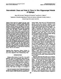
The circuit used to model (8) is shown in ®gure 1. The basic principles of the circuit design can be found in [59, 61 ± 64]. We use superscript primes to distinguish times and frequencies in the circuit (in units of s and Hz) from the corresponding dimensionless times and frequencies that appear in equation (8). To understand the relationships between quantities in the circuit and in (8), we sum the currents at point A, and those at point B, and equate them to zero in each case (using KirchhoV’s law and the assumption of in®nite input impedance of an operational ampli®er). The equations for the points A and B are respectively C

dV2 ‡ 1 0 … 0 † ‡ 1 0 1 0 0 x t h cos …O t † ‡ V1 ˆ 0; 0 dt R1 R R2 1 1 1 V1 ‡ V2 ‡ V3 ˆ 0: 10R 10R R

Noting (see ®gure 1) that 3

V2 V3 ˆ ¡ 10 it is straightforward to show that R1 C

dV2 ‡ 0 … 0 † ‡ R1 3 ¡ R1 R1 0 0 0 x t V2 V2 ‡ h cos …O t † ˆ 0: 0 dt R2 R2 R

0 By making the transformations V2 ! x; t ! tt; 0 0 x …t † ! x…t†, and choosing the circuit component values

R1 ˆ R2 ˆ R ˆ 10kO; C ˆ 10nF; t ˆ CR1 ; we then arrive at equation (8). We drive the circuit with zero-mean quasi-white Gaussian noise from a shift-register noise generator, and with a periodic signal from the HP signal generator. Starting with the system in the close vicinity of one of the stable states …xi º §1†, successive blocks of x(t) time series were digitized and examined. Note that the time in all the ®gures was measured in units of ½ ˆ 100ms and coordinates and velocities are measured in volts. However, dimensionless coordinates that appear in the equations may represent diVerent physical quantities including, for example, posi-

Deterministic patterns of noise and the control of chaos

383

Figure 1. Block diagram of an analogue electronic circuit modelling an overdamped double-well Du ng oscillator (equation (8)) either with, or without, the periodic force h ’ cos O ’t ’.

tion of the Brownian particle, intensity of light in lasers, and number of species in chemical reactions. That is why the ®gures use dimensionless coordinates and time that appears in the equations of motion.

2.4.

Example from ecology

Note that the idea of continuous monitoring of dynamical variables and driving forces is not entirely new. For example in forest ecology [65] the frequency of ®res and the area burned (that can be considered as dynamical variables) and the weather parameters (that can be considered as driving forces with periodic and random components) have been monitored continuously for some forests for more than a century. In the context of forest ecology large ¯uctuation of a dynamical system corresponds to a large ®re. Interestingly enough historical data collected by forest ecologists have led them to the conclusion [66] that: the climate for a year or more preceding ®res in¯uences ecological eVects during extended droughts . . . extended droughts also set the stage for ®res that consume most of the organic layer. Thus we see that large deviations in the weather parameters that are analogous to the optimal force drive the occurrence of large ®res by setting extended droughts that are analogous to the optimal paths along which the forest is evolving towards large ®res.

However, the reality is far more complicated than the simple qualitative arguments discussed above. Many diVerent processes in¯uencing fuel accumulation and consumption in diVerent types of forests have to be taken into account to reveal quantitative relations between parameters characterizing a ®re’s succession. The corresponding research is currently under way. To guide researchers through the complexity of the possible stochastic dynamical behaviour it is very useful to analyse in detail the stochastic dynamics of large ¯uctuations in simpler dynamical models as described in the following sections.

2.5.

Time symmetry of ¯uctuations

Let us now verify by experiment Onsager’s proposition about the symmetry between average growth and average decay of ¯uctuations for a system in thermal equilibrium. To do so one can use, for example, the analogue electronic circuit described in the previous subsection and set the amplitude of the driving force to zero (see also [60, 67] for the details of how similar experiments can be performed in lasers). To compare directly in the experiment the laws of average growth and average decay of ¯uctuations one has to collect an ensemble of the actual ¯uctuational trajectories moving the system from the equilibrium state to the remote state and back to equilibrium. The corresponding

384

D. G. Luchinsky

distribution of the ¯uctuational trajectories that include both relaxational and ¯uctuational parts we denote for brevity pf(x, t) (see [36, 58, 59] for details). Examples of trajectories including ¯uctuational and relaxational parts as observed in an analogue electronic circuit are shown in ®gure 2(a). The corresponding model is an overdamped motion of a Brownian particle x_ ˆ f…x† ‡ x…t†; 5x…t†4 ˆ 0; 5x…t†x…0†4 ˆ Dd…t†; …10† 2 4 in a Du ng potential U(x) ˆ ¡ x /2+x /4, f(x) ˆ ¡ U’(x). The distribution pf(x, t) build from an ensemble of such trajectories is shown in ®gure 2(b). To compare these results with the theoretical prediction, notice that the Hamilton ± Jacobi equation in this case takes the form 2 H ˆ 1/2p +f(x)p ˆ 0. And the Hamiltonian equations of 0 00 motion are x_ ˆ p ¡ U …x†; p_ ˆ pU …x† (cf section 2.1 and [36, 38]). Two solutions of the Hamilton ± Jacobi equation, p ˆ 0 and p ˆ ¡ 2f(x), correspond to the relaxational …x_ ˆ ¡U0 …x†† and ¯uctuational …x_ ˆ ‡U0 …x†† deterministic paths respectively. It can be seen from ®gure 2 that the ridges of the distributions coincide with the optimal paths predicted by the theory thus demonstrating time-reversed symmetry between average growth and average decay of ¯uctuations. Note that although the system (10) is relatively simple, it describes very well the ¯uctuational dynamics of many real physical systems. In particular, a behaviour qualitativel y similar to the one shown in ®gure 2 was observed recently in experiments with semiconductor lasers [60, 67]. In the work by Hales and co-authors [60] the prehistory distribution was observed experimentally using a semiconductor laser with optical feedback. Near the solitary threshold, the system was unstable: after a period of nearly steady operation, the radiation intensity decreased; then it recovered comparatively quickly, growing to regain its original value; decreased again; and the cycle repeated. In the experiment, the output intensity was digitized with 1 ns resolution and the prehistory probability density of large ¯uctuations near solitary threshold was built. The results were in agreement with the results of numerical simulation for the system (10). In the work by Willemsen and co-authors (see [67] and references therein) the three Stokes polarization parameters were studied during polarization switches in a verticalcavity semiconductor laser. It was demonstrated that when the linear part of the absorptive anisotropy is close to zero, the laser is bistable and switches stochastically between two polarizations . The analysis of large ¯uctuations of polarizations in the system [67] reveals what authors have called a `stochastic inversion symmetry’, which is analogous to the time reversal symmetry observed for the model (10) and shown in ®gure 2.

We now turn to experimental methods of investigation of momenta.

2.6.

An optimal force

The physical meaning of the momenta in equations (7) has been the subject of dispute in the literature. For example in the paper [46] it is noted that the momentum p determines the D ! 0 limit of the logarithmic gradient of the stationery probability density and can be interpreted as a measure of the extent to which optimal trajectories move against the deterministic drift f. An important idea by Dykman [29] is that momenta are ultimately related to the optimal ¯uctuational force corresponding to the optimal path and thus they can be also sometimes measured experimentally as ensemble average of the realizations of the random force corresponding to a given optimal path. This point is often glossed over in the theoretical literature, with some authors describing p as a mere theoretical abstraction. In the particular case of analogue experiment or numerical simulations, where the noise is external and thus is accessible to measurement, the momentum can be identi®ed as the averaged value of the force driving the ¯uctuation. We have therefore performed simultaneous measurements [37] of x(t) and of the random force x(t) in the system (10) during transitions between potential wells. The paths traced out by the ridges of the distribution of the realizations of random force pf(p,t) are shown in ®gure 3 as compared to the theoretically predicted trajectories. Note that even in thermal equilibrium Hamiltonian theory envisages the ¯uctuational and relaxational trajectories as belonging to two diVerent manifolds of the system (10), with p ˆ 2U’(x) and p ˆ 0 respectively. The direct experimental measurements of the momenta demonstrate quantitative agreement with the theory. We conclude that the momenta appearing in the Hamiltonian theory of ¯uctuations are physically observable. Further insight into the physical meaning of the momenta will be provided in section 3.2. Note that for the system in thermal equilibrium considered so far the time symmetry between average growth and average decay of ¯uctuations simpli®es considerably investigation s of the optimal paths. In particular, this symmetry implies that optimal paths can be found from an analysis of the relaxation and thus they cannot display any singular behaviour. However, away from thermal equilibrium the time reversal symmetry is broken and as a result the patterns of the optimal ¯uctuational paths may display singularities. Thus understanding ¯uctuations in systems away from thermal equilibrium requires investigation of the patterns of the optimal ¯uctuational paths and analysis of the correspond-

Deterministic patterns of noise and the control of chaos

385

Figure 2. (a) The coordinate of an overdamped Du ng oscillator x(t) was monitored continuously, waiting for large ¯uctuations reaching a chosen preset voltage threshold representing xf . Fluctuational paths x (t) reaching xf were preserved for later analysis, and so also were the relaxational paths from xf back towards the stable state at x ˆ ¡ 1. Two typical ¯uctuations (jagged lines) from the stable state at x ˆ ¡ 1 to the remote state x f ˆ ¡ 0.1, and back again, are compared with the deterministic (noise-free) relaxational path from xf to the stable state (full, smooth, curve) and its time-reversed (t? ¡ t) mirror image (dashed curve). The ¯uctuational and relaxational parts of the trajectory are labelled f and r respectively. (b) The probability distribution p f (x,t) built up by ensemble-averaging a sequence of trajectories like those in ®gure 1. The topplane plots the positions of the ridges of pf (x ,t) for the ¯uctuational (yellow squares) and relaxational (green circles) parts of the trajectory for comparison with theoretical predictions (curves) based on a Hamiltonian approach. Time t in both ®gures is given in units of integration time of the electronic circuit t ˆ 100 m s and the coordinates are in volts (see section 2.3 for a discussion.)

ing singularities. These ideas can be illustrated by analysing overdamped motion of a Brownian particle in a periodically driven potential as the simplest nontrivial example of the system away from thermal equilibrium.

2.7.

Periodically driven system

Let us consider the stochastic dynamics of the following system x_ ˆ f…x; t† ‡ x…t†; 0

Figure 3. Results of measurements of the optimal force. The inset shows p(x) for two typical transitional trajectories from x ˆ ¡ 1 to x ˆ 1 (full jagged line). The main ®gure shows the paths traced out by the ridges of the pf(p,x) distribution built as an ensemble average of such transitional trajectories in the phase space of the system (10). The ¯uctuational part from x ˆ ¡ 1 to x ˆ 0 is shown by yellow squares, and the relaxational part by green circles. The full blue and red curves are the corresponding paths predicted by the Hamiltonian theory. See section 2.3 for a discussion of the units for coordinates and momenta.

…11†

where f…x; t† ˆ ¡U …x† ‡ h cos Ot is deterministic force, U…x† ˆ ¡x2 =2 ‡ x4 =4 is the Du ng potential, and x(t) is a zero-mean white Gaussian noise as above. This system was investigated in a broad variety of application s in the context of stochastic resonance [18 ± 21]. Note that the only diVerence from the previous case is the addition of periodic driving. However, in the presence of a periodic force with frequency close to the inverse relaxation time of the system (11) no general methods exist to ®nd a solution of the Fokker ± Planck equation. The corresponding problem of so-called non-adiabatic driving is a well-known longstanding unsolved problem of the theory of ¯uctuations [68, 69]. The Hamiltonian theory of ¯uctuations provides a powerful approach to the numerical analysis of this problem [59] (see also [70, 71] for alternative numerical approaches).

D. G. Luchinsky

386

Equations (6) and (7) in this case take the form @S ‡ ˆ @S ‡ … † ‡ 2 ˆ H pf x; t p =2 0; @t @T

…12†

1 2 0 …13† x_ ˆ f…x; t† ‡ p; p_ ˆ ¡f …x; t†p; S_ ˆ p ; 2 0 where f …x; t† ˆ @f…x; t†=@x. Unlike in the previous case of a one-dimensional system in thermal equilibrium an analytical solution cannot be obtained. The numerical integration of equations (13) requires a knowledge of the initial conditions. In the general case the initial conditions can be found by a perturbation procedure [42, 49] (see, however, the discussion of a chaotic state in the next section). For system (12) we have (see Dykman et al. [31]) x ˆ xd …t† ‡ dx; S ˆ 1=2a…t†dx2 ; p ˆ a…t†dx;

…14†

where xd (t) is the point on the deterministic trajectory at time t, dx is a small time-independent deviation from xd (t), and the periodic function a(t) is a second derivative of the action at this point that satis®es the equation 0 a_ ˆ ¡2f …x; t†a ¡ a2 . It is known [72] from the theory of dynamical systems that the trajectories found by solving (13) with initial

conditions (14) form a one-parameter set (x(t,dx), p(t,dx)) lying on a Lagrangian manifold (LM) in t, x, p-space. The corresponding manifold is shown in ®gure 4. The projection of these trajectories on the coordinate t, xplane form the extreme paths shown at the bottom of ®gure 4 and in ®gure 5(a). It is evident from these ®gures that the pattern of optimal paths is periodic in time and that for each period there is one most probable escape trajectory, i.e. trajectory connecting the stationary periodic state (at t? ¡ ?) with the stable state (at t??). Several extreme paths may arrive from the stationary periodic state xd (t) to the same remote state. And, in general, computation of S requires minimization over the set of all trajectories starting at the stable state and terminating at a given remote state. It is also known that the only types of singularities that occur in the system (13) are folds of the LM emerging in pairs from the cusp point and giving rise locally to a swallow-tail singularity of the action surface [31, 72] (see ®gure 4). Topological [73] and numerical [54] analysis shows that in the D?0 limit the only observable singularities in the corresponding patterns of the pattern of extreme paths are cusp and so-called switching line, a singularity separating regions that are approached via diVerent ¯uctuational paths. The switching lines are

Figure 4. From top to bottom: Lagrangian manifold (LM); action surface; and extreme paths calculated [59] for the system (11) using equations (13). The parameters for the system were h ˆ 0.264 and O ˆ 1.2. To clarify interrelations between singularities in the pattern of optimal paths, action surface, and LM surface, they are shown in a single ®gure, as follows: the LM has been shifted up by one unit; and the action surface has been scaled by a factor 1/2 and shifted up by 0.4.

Deterministic patterns of noise and the control of chaos

projections of the intersection of the two lowest sheets of the action surface onto the t, x-plane. The nontrivial features of the pattern of optimal paths, including occurrence of the switching line and of the cusp, can be tested experimentally [31, 56, 58, 59] using the technique described in the previous section. Figure 5(b) shows as an example the measured pf(x,t) when xf is placed on the calculated switching line [56]. It can be seen that the ridges of the distribution are strongly asymmetric in time, but agree well with the ¯uctuational and relaxational paths predicted from (13). Note that the observed asymmetry of the distribution implies [74] a lack of detailed balance, and leads directly [47, 48] to macroscopic irreversibilit y in the D?0 limit where the width of the distribution tends to zero. In verifying the existence of the switching line, the results demonstrate the non-di Verentiability of the generalized non-equilibrium potential [54, 55] discussed in section 2.2.

2.8.

The theory of logarithmic susceptibility

Perhaps one of the most interesting examples of how the knowledge of the optimal paths can advance our understanding of ¯uctuations in periodically driven systems is the recent development of the theory of logarithmic susceptibility (LS) [75, 76]. This theory describes the eVect of a comparatively weak ®eld on the escape probability in terms of the work that the ®eld does on the system as it moves along the optimal path. This approach leads to the analytical solution [77] of the non-adiabatic escape problem (11) described in the beginning of this subsection. It follows from the theory that in the case of periodic driving F…t† ˆ h cos…Ot†, the leading-order correction dR to the activation energy of escape is dR ˆ ¡jÀ…O†jh, where the logarithmic susceptibility w(O) for the escape is given [75, 76] by the Fourier transform of the velocity along the most probable escape path in the absence of driving (F(t) ˆ 0). We have already noted that, for systems in thermal equilibrium, optimal ¯uctuational paths are the time-reversed relaxational paths in the absence of noise [44, 57, 78]. The LS theory was used recently to describe the localization of a Brownian particle in a three-dimensional optical trap [79]: a transparent dielectric spherical silica particle of diameter 0.6 mm suspended in a liquid [80]. The particle moves at random within the potential well created with a gradient three-dimensional optical trap. The potential was modulated by a biharmonic force. By changing the phase shift between the two harmonics it was possible to localize the particle in one of the wells in very good quantitative agreement with the theoretical predictions. Another important application of the LS theory is the analysis of the dynamics of Brownian ratchets. The term `Brownian ratchets’ is used to describe systems that display

387

a unidirectiona l diVusion of the Brownian particles in a periodic potential when the net force (averaged over the period of driving) acting on the particle is zero. Such systems have attracted recently considerable attention in view of their technological application s and as possible models describing motion of molecular motors (see the Introduction). The LS theory predicts, in particular, the occurrence of resonant activation, recti®cation of ¯uctuations, and current reversal in an asymmetric periodic potential in the presence of external periodic driving [75]. These predictions were recently con®rmed in analogue electronic experiment [81]. The last two examples illustrate how a knowledge of the optimal paths can help to control ¯uctuational dynamics in non-equilibriu m systems by applying an external ®eld. This brings us close to the subject of the next section where an application of the Hamiltonian theory of ¯uctuations to control theory is considered. Such application s are based on simultaneous measurements of the optimal force and of the optimal paths described in this section. These measurements pave the way for direct experimental investigation s of the structure of the Lagrangian manifold underlying the dynamics of a system in the presence of ¯uctuations or in the presence of the control, even when theoretical predictions are not available. Therefore we suggest that our technique can be used to advance some unsolved problems in the theory of ¯uctuations and in the control theory. In particular, in the work by Dykman and Smelyanskiy [82] it was also noted that the optimal ¯uctuational force can sometimes be identi®ed with the control function. These ideas will be further discussed in the following section.

3.

The problem of the control of chaos

The problem of the control of chaos is a subject of broad interdisciplinar y interest, both from the point of view of application s and for fundamental research [83]. The methods available for the control of chaos are diverse [83, 84] and include entraining to some arbitrary `goal dynamics’ that necessarily require large modi®cations of the system’s dynamics [85, 86] and a variety of `minimal’ forms of interaction [89 ± 92] that are restricted by the linear approximations adopted. However, the energy-optimal implementation of switching from the basin of attraction of a chaotic attractor (CA) has remained an unsolved archetypal problem [91] for a long time. Its solution will extend very substantially the variety of model-exploratio n objectives (cf [85] and [89]) that can be achieved by `minimal’ forms of control. At the same time, the question of stability of a CA in the presence of noise has remained a major scienti®c challenge ever since the ®rst attempts to generalize the classical escape problem to cover this case [94 ± 97].

D. G. Luchinsky

388

The two problems mentioned above are usually considered separately within the two distinct ®elds of deterministic and stochastic nonlinear dynamics. Here we discuss how they can be addressed via a novel approach based on an analogy between the Hamiltonian formulations of both problems and the statistical analysis of the ¯uctuational trajectories. The di culty in solving these problems stems from the complexity of the system’s dynamics near a CA and is related, in particular, to the delicate problems of the uniqueness of the solution and the boundary conditions at a CA (cf with the discussion of the problem of initial conditions in section 2.7). The approach we are going to adopt is based on the fact that the Wentzel ± Freidlin Hamiltonian arising in the problem of ¯uctuations (see section 2.2) is equivalent to Pontryagin’s Hamiltonian that arises in the control problem [91] with an additive linear unrestricted control. The optimal control function in this case is equivalent to the optimal ¯uctuational force [82].

3.1.

Model

Consider the motion of a periodically driven nonlinear oscillator: x_ 1 ˆ f1 ˆ x2 ; x_ 2 ˆ f2 ˆ ¡2Gx2 ¡ o20 x1 ¡ bx21 ¡ gx31 ¡ h cos …Ot† ‡ u…t†: …15† Here u(t) is the control function. Parameters were chosen such that the potential is monostable …b5Go20 †, the dependence of the energy of oscillations on their frequency b2 9† is nonmonotoni c …Go2 4 10 , and the motion is under0 ½ º O 2o0 . This model is of interest in a damped G number of contexts and the theoretical analysis is possible for a wide range of parameter values [96]. It is a system in which chaos can be observed at relatively small values h&0.1 of the driving force amplitude. For a given damping (G ˆ 0.025) the amplitude and the frequency of the driving force were chosen so that the chaotic attractor coexists with the stable limit cycle (S1 in ®gure 6(b)). This regime is often encountered in applications which are of practical interest [12, 97, 98]. The chaotic state appears via period-doublin g bifurcations as shown in the ®gure 6(a) and thus corresponds to a non-hyperboli c attractor. Its boundary of attraction dO is nonfractal and is formed by the saddle cycle of period 1 (SC). For details about the phase diagram see [99]. We have considered the following energy-optimal control problem. The system (15) with unconstrained control function u(t) is to be steered from the CA to the stable limit cycle in such a way that the energy (cost) functional R is minimized, with t1 unspeci®ed

R ˆ inf

Z

t1 t0

1 2 f0 …x; t†dt; f0 …x; t† ˆ u …t†: 2

…16†

Here the control set U consists of functions (control signals) able to move the system from the CA to the SC.

3.2.

Analogy between two problems

It can be shown [91] that, if a solution of the control problem …u…t†; x…t†† exists, then there also exists a continuous piece-wise diVerentiable function P ˆ p(t) {p1(t), p2(t)} such that Hc ˆ iˆ0;2 pi fi . Here Hc is the so-called Pontryagin’s Hamiltonian, the variables p1(t), p2(t) are not simultaneously zero, p0 is constant 50. If the optimal control function u…t† at each instant takes those values u(t) ˆ p2 that maximize Hc over U, the corresponding equations of motion for this problem take the form Hc ˆ 1=2p22 ‡ p1 f1 ‡ p2 f2 ; @Hc @Hc x_ i ˆ ; p_ i ˆ ¡ ; i ˆ f1; 2g: @pi @xi

…17†

It can be seen that Hc in (17) coincides with the Wentzel ± Freidlin Hamiltonian in (6) if the control signal u(t) in (15) is substituted with zero-mean white Gaussian noise x(t) such that x ‡ 2Gx_ ‡ o20 x ‡ bx2 ‡ gx3 ‡ h cos …Ot† ˆ x…t†; hx…t†i ˆ 0; hx…t†x…0†i ˆ 4GkTd…t†

…18†

and Qij ˆ di2dj2 in equation (6). Thus the optimal control signal u…t† can be identi®ed with the optimal ¯uctuational force [82] that drives the system from the CA to the SC. We note that both u…t† and the optimal force are related to p2 in (17). An analysis of the analogy between two problems requires a more general formulation of the stochastic control problem which goes beyond the scope of the present paper (see [84, 102 ± 104] and references therein). Here we provide some additional semi-qualitativ e arguments to illustrate this idea. This interrelationshi p is intuitively clear because, in thermal equilibrium (D ˆ 4GkB T), the probability of ¯uctuations is determined by the minimum work from the external source needed to produce the corresponding change in the thermodynamic quantities r / exp…¡Rmin =kB T† [40] and for the system (15) Rmin is given by R in (16). On the other hand the same probabilit y is given by the optimal realization of the random force x(t) minimizing integral in the probabilit y density functional Rt 1 2 P‰x…t†Š / exp…¡1=8GkT t0 x …t†dt† [44, 51]. On substituting x(t) from (18) and u(t) from (15) into this integral we obtain the same variational problem in both cases. We

Deterministic patterns of noise and the control of chaos

389

Figure 5. (a) The pattern of the extreme paths forming unstable manifold of the stable state of system (11) with h ˆ 0.1, O ˆ 4.0 is shown by thin blue solid lines. The most probable escape trajectories (see the text) are shown by thick solid lines. The stable and unstable periodic states are shown by yellow and red circles respectively. (b) The measured prehistory distribution pf(x,t) for a remote state xf ˆ ¡ 0.63, t ˆ 0.83 that lies on the switching line of system (11) with h ˆ 0.264, O ˆ 1.2. Fluctuational (yellow circles) and relaxational (red circles) paths determined by tracing the ridges of the distribution, are compared with the corresponding (black solid) theoretical lines predicted from (13) at the top of the ®gure. The stable and unstable states are shown by the dashed black line. See section 2.3 for a discussion of the units for coordinates and momenta.

Figure 6. (a) A phase-parametric diagram for the system described by equation (15) in Poincare cross-section obtained with Ot ˆ 0(mod2 p), O ˆ 1.005 shows values of x1 for diVerent h. The region of hysteresis for the period 2 resonance lies between the arrows 1 and 4. The region of coexistence of the two resonances of period 2 lies between arrows 2 and 5; that of the large stable limit cycle of period 1 lies between arrows 3 and 9. Arrows 6 ± 9 show the boundaries of the chaotic states. (b) The basin of attraction (shaded red) of the stable limit cycle S1 (black circle) and that of the chaotic attractor CA (white) in Poincare cross-section with Ot ˆ 0.6p(mod2p), O ˆ 0.95. The boundary SC of the CA’s basin of attraction, the saddle cycle of period 1, is shown by the black square. The saddle cycle of period 3 is shown by black pluses. The intersections of the actual escape trajectory with the Poincare cross-section are indicated by the blue circles.

D. G. Luchinsky

390

therefore suggest that the optimal control function u…t† can be found by applying experimental technique described in the previous section. 3.3.

Escape from a chaotic attractor

The idea that the energy-control of chaos can be eVected via statistical analysis of the ¯uctuational trajectories has been tested through analogue electronic modeling of (15) and digital simulation following the prescriptions of [103]. Qualitatively similar results were obtained but, because precision is of particular importance here, most of the data reported here are those from the digital simulations. The underlying mechanism is that, when the system (15) is driven by a random force x(t) instead of u(t), it will occasionally ¯uctuate to dO. In doing so in the limit where the noise intensity tends to zero, the system will follow very closely the deterministic trajectories of (17). For the technique to be applicable a solution of (17) moving the system from the CA to dO must exist, and the boundary conditions for this solution on the CA must be identi®ed. As described in the previous section the method involves monitoring the system continuously and collecting all esc successful realizations …xesc …t†; x_ esc …t†; x …t†† moving it from the CA to dO. One of actual escape trajectories is indicated in Poincare cross-section by the blue ®lled circles in ®gure 6(b). From these realizations, a time-dependent prehistory distribution is built [37]. The typical situation as measured in the analogue simulations is shown in ®gure 7. The ®gure shows 65 measured ¯uctuational escape trajectories, each of which has been shifted in time so that the regions corresponding to the transition from chaotic to regular motion coincide with each other. It is evident that all the trajectories end up close together, passing through the immediate neighbourhoo d of psome     optimal trajectory within a tube of radius / D; at earlier times, however, they separate into distinct groups. The number of optimal trajectories of the transition CA?S3 depends on the choice of the working point. If the noise intensity is reduced further, one of the escape paths becomes exponentiall y more probable than all the others. In what follows we concentrate on the properties of this most probable escape path. A typical optimal escape path and the corresponding optimal force, obtained by averaging a few hundred such trajectories, are shown in ®gure 8(a). Analysis of the optimal path reveals that the system leaves the CA along the unstable manifold of the saddle cycle of period 5 (S5 with multipliers m1 ˆ 0.0415751 and m2 ˆ 4.60403728 41) embedded in the CA. At this moment the optimal esc ¯uctuational force hx …t†i switches on, driving the

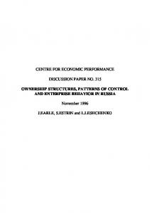
system to dO via the saddle cycle of period 3 (S3 with multipliers m1 ˆ 0.0487351 and m2 ˆ 7.608312 41). It can be seen from ®gure 6(b) that the saddle cycle S3 is not embedded in the CA. It is probably the nearest saddle cycle to the boundary of the basin of attraction of the CA in terms of the action variable, and can be considered as the boundary of the CA itself. Near the saddle cycle SC that forms the boundary of the basin of attraction the optimal force dies out. Note that no action is required to bring the system from S1 to the stable limit cycle. As discussed above, this path is an approximatio n (because of the ®nite intensity of the noise) to the optimal control function u…t†. The form of the boundary conditions is one of the central results of the analysis. The boundary conditions are found by analysis of how the energy-optimal escape path …hxesc … †i h esc … †i† merges with the CA as shown in ®gure 1 t ; x2 t 8(b). It can be inferred that most of the escape trajectories pass close to the saddle cycle of period 5 embedded in the CA. This inference can be further elaborated by reducing the noise intensity as explained in [104]. Note that the topological features of the prehistory distribution yield direct insight into the control problem: where the prehistory distribution does not develop a wellde®ned ridge in the D?0 limit, we may infer that control via a simple function is not achievable. In the present case, this distribution turns out to be characterized by a narrow ridge, as the noise intensity is decreased, allowing us to de®ne an approximate solution uÄ(t) for the control function (the exact solution is u…t† ˆ limD !0 u~…t†), as an ensemble esc average hx …t†i of the realizations of the random force corresponding to the energy-optimal escape path (of section 2.6). Thus we conclude that the solution uÄ(t) and the corresponding boundary conditions can be found using our new experimental method. Moreover the escape problem has in this case been reduced to the analysis of transitions between three saddle cycles S5?S3?SC, in qualitative agreement with the well-known statement that saddle cycles provide detailed invariant characterizations for dynamical systems of low intrinsic dimension [105, 106]. We note that the solution found is independent of the initial conditions on the chaotic attractor: the transient time required for the system to reach S5 (in the presence of noise) from arbitrary initial conditions is exponentially smaller than average escape time; and the quasi-periodi c steady state distribution is formed on the attractor prior to escape [104]. Once boundary conditions are speci®ed one can solve the corresponding boundary value problem for the system (17) numerically [104]. The results of the numerical solution of the boundary value problem obtained by the relaxational method are shown in ®gure 8(a) by the dotted lines and are

Deterministic patterns of noise and the control of chaos

391

Figure 7. Escape trajectories (black lines) found in the analogue simulations for the parameters h ˆ 0.19, O&1.045, o0 &0.597, T&0.005. The red triangles show the calculated saddle cycle of period 1 at the boundar y of the basin of attraction. The back-plane shows for comparison the Poincare cross-section and the basins of attraction chaotic attractor (blue-shaded) and stable limit cycle (white) for Ot ˆ 0. The red ®lled circle and the black ®lled square indicate, respectively, the intersections of the stable limit cycle and saddle cycle with the Poincare section. Time is measured as a number N of periods T ˆ 2p/O of the driving force. See section 2.3 for a discussion of the units for coordinates.

Figure 8. (a) Main ®gure: the most probable escape path (full blue curve) from S5 to SC, found in the numerical simulations. Single periods of the unstable saddle cycles of period 5, 3 and 1 are shown by green circles, black squares and mauve triangles respectively; the stable limit cycle is shown by blue rhombus. The parameters were h ˆ 0.13, O&0.95, o0 &0.597, D&0.01. Inset: the optimal force (full blue curve) corresponding to the optimal path, after ®ltration. The red-dotted line in both parts of the ®gure is from a numerical solution of the boundary value problem. (b) Contour plot of the prehistory probability distribution of escape trajectories for the same parameters as in ®gure 7. The colours of the contour plot show relative intensity (in arbitrary units) of the prehistory distribution as indicated by the colourbar on the right-hand side. The blue squares show one period of the saddle cycle S3. The black circles, showing one period of S5, have been displaced vertically in the interests of clarity. The red triangles indicate the stable limit cycle. Time is measured as the number N of periods T ˆ 2p/O of the driving force as in the previous ®gure.

392

D. G. Luchinsky

in a good agreement with the solution found from the analysis of ¯uctuational trajectories.

3.4.

Energy-optimal entraining of the chaotic attractor

To demonstrate that the optimal force uÄ(t) found in the experiment really does minimize the energy of the control function steering the system (15) from the CA to the SC we set it to arbitrary initial conditions in the basin of attraction of the CA and let it evolve deterministically until it passed through the initial part of the unstable manifold of S5. At this moment the deterministic control function was switched on. For a given shape of the control function and/or initial conditions, its amplitude was set to the threshold for switching of the system from chaotic to regular motion on SC. It was found that the system is very sensitive to small variations in the control function: any deviation from the shape of uÄ(t), or from the initial conditions found in the experiment, leads to a substantial increase in the energy required to attain SC. Some experimental results are shown in ®gure 9. It can be seen that the energy of the control function is approximately twice as large if the optimal force is approximate d by the sine function modulated by a Gaussian 2 u…t† ˆ a1 sin …a2 t† exp …¡…t ¡ a3 † a4 †, and it is respectively ¹4 and ¹20 times larger if the optimal force is approximated by rectangular pulses or distorted with an arbitrary lowfrequency perturbation. We have also performed experiments using an open-plusclosed-loop control technique [85] and an adaptive control algorithm [86] to steer the system from the CA to the SC. Although these methods are designed to optimize the recovery time, rather than to minimize the energy of the control function, they are e cient in entraining the system dynamics to the goal dynamics. So it is interesting to compare their performance with that of the control function found in our experiment. The energy of the control functions (see ®gure 8(a)) obtained by these methods is more than an order of magnitude larger than the energy of the optimal control function u(t) found by our new technique. The best results obtained by the open-plusclosed-loop control are also shown in ®gure 9. Of course, the time required for the system to approach S5 (which is where the optimal control force can be switched on) varies for diVerent initial conditions on the D CA: it is typically e p, where e is the linear dimension of the region and the Dp is the pointwise dimension of a periodic point in this region [106]. In order to reduce this initial waiting period, and thus the average transition time, one could apply the techniques [90, 107] developed earlier for eVecting switching between controlled saddle periodic orbits embedded in an CA. In conclusion, a novel technique for the energy optimal steering of a nonlinear oscillator away from the

Figure 9. (a) The control functions (not to the same scale) used in the numerical experiments: 1 Ð optimal force found by statistical analysis of the ¯uctuational escape trajectories; 2 Ð approximation of the optimal force by u(t) ˆ a1 sin(a2 t) 2 exp(-(t-a3 ) a4 ) where ai are constants; 3 Ð approximation of the optimal force by rectangular pulses; 4 Ð arbitrary perturbation of the optimal force with a low-frequency perturbation; 5 Ð control functions produced by the OPCL (open-plusclosed-loop) algorithm. (b) Energies of the control functions shown in (a).

basin of attraction of an CA have been proposed and veri®ed experimentally. The technique is based on statistical analysis of the ¯uctuational trajectories in the control-free system. It can readily be combined with established minimal forms of control, extending substantially the range of model-exploratio n objectives that can be achieved by such methods. We infer that it can be further extended to treat cases where the boundaries of attraction are fractal. The obtained results open the possibility of the analytical estimations of stability of non-hyperboli c attractors in the presence of ¯uctuations.

Deterministic patterns of noise and the control of chaos

4.

Conclusions

An idea to describe highly irregular stochastic motion in terms of deterministic motion along trajectories of auxiliar y Hamiltonian system is often the key to understanding ¯uctuational dynamics away from thermal equilibrium. This idea underlies the recent rapid advances in the theory of ¯uctuations. The optimal ¯uctuational paths, that appear formally in the asymptotic analysis of the Fokker ± Planck equation (or, alternatively, in the path-integral formulation of the problem of ¯uctuations), are physically observable. The introduction of the prehistory probability distribution, have set the area on an experimental basis for the ®rst time, and helped to stimulate new advances in the theory. These have included the logarithmic susceptibility, described above, which provided analytical solution to the long-standin g problem of non-adiabatic driving. Studies of the ¯uctuational escape from chaotic attractors have already provided strong guidance for future developments in the theory. It seems certain that the emergence of many new results and phenomena may be anticipated over the new few years.

[11] [12] [13] [14] [15] [16] [17] [18] [19] [20]

[21] [22] [23] [24] [25] [26] [27] [28]

Acknowledgements I warmly acknowledge the assistance and support of my many collaborator s in the research reviewed in this paper including, especially, M.I. Dykman, I.A. Khovanov, P.V.E. McClintock, R. Maier, R. Mannella, V.N. Smelyanskiy, S.M. Soskin, N.D. Stein, D. Stein and N.G. Stocks. The research has been supported in part by the Engineering and Physical Sciences Research Council (UK), INTAS, the EC, the Royal Society of London, by Award No. REC ¡ 006 of the U.S. Civilian Research Development Foundation for the Independent States of the Former Soviet Union (CRDF), and RFFI.

[29] [30] [31]

[32]

[33]

[34]

References [1] Lindenberg, K., and West, B. J., 1990, The Nonequilibrium Statistical Mechanics of Open and Closed Systems (New York: VCH). [2] Einstein, A., 1905, Ann. d. Phys., 17, 549. [3] Langevin, P., 1908, Comptes. Rendues, 146, 530. [4] Feynman, R. P., Leighton, R. B., and Sands, M. L., 1965, The Feynman Lectures on Physics, volume 1 (Massachusetts: AddisonWesley). [5] Magnasco, M. O., 1993, Phys. Rev. Lett., 71, 1477 ± 1481. [6] Bier, M., 1997, Cont. Phys., 38, 371 ± 379. [7] Visscher, K., Schnitzer, M. J., and Block, S. M., 1999, Nature, 400, 184 ± 189. [8] Soong, R. K., Bachand, G. D., Neves, H. P., Olkhovets, A. G., Craighead, H. G., and Montemagno, C. D., 2000, Science, 290, 1555 ± 1558. [9] Kawaguchi, I., and Ishiwata, S., 2001, Science, 291, 667 ± 669. [10] Johnson, J., 1928, Phys. Rev., 32, 97 ± 109.

[35] [36] [37] [38] [39]

[40] [41] [42] [43] [44] [45]

393

Nyquist, H., 1928, Phys. Rev., 32, 110 ± 113. Kautz, R. L., 1987, Phys. Lett. A, 125, 315 ± 319. Kramers, H., 1940, Physica (Utrecht), 7, 284 ± 304. Hanggi, P., Talkner, P., and Borkovec, M., 1990, Rev. Mod. Phys., 62, 251 ± 341. Mel’nikov, V. I., 1991, Phys. Rep., 209, 1 ± 71. Benzi, R., Sutera, A., and Vulpiani, A., 1981, J. Phys. A, 14, L453 ± L457. Hays, J. D., Imbrie, J., and Shackleton, N. J., 1976, Science, 60, 1121. Moss, F., and Wiesenfeld, K., 1995, Scienti®c American, 273, 66 ± 69. Bulsara, A. R., and Gammaitoni, L., 1996, Physics Today, 49, 39 ± 45. Dykman, M. I., Luchinsky, D. G., Mannella, R., McClintock, P. V. E., Stein, N. D., and Stocks, N., 1995, Nuovo Cimento D, 17, 661 ± 683. Gammaitoni, L., HaÈnggi, P., Jung, P., and Marchesoni, F., 1998, Rev. Mod. Phys., 70, 223 ± 287. McNamara, B., Wiensenfeld, K., and Roy, R., 1988, Phys. Rev. Lett., 1, 3 ± 4. Dykman, M. I., Velikovich, A. L., Golubev, G. P., Luchinsky, D. G., and Tsuprikov, S. V., 1991, Sov. Phys. JEPT Lett., 53, 193 ± 197. Douglass, J., Wilkens, L., Pantazelou, E., and Moss, F., 1993, Nature, 365, 337 ± 441. Leonard, D. S., and Reichl, L. E., 1994, Phys. Rev. E, 49, 1734 ± 1737. Wallace, R., Wallace, D., and Andrews, H., 1997, Environment and Planning A, 29, 525 ± 555. Feynman, R. P., and Hibbs, A. R., 1965, Quantum Mechanics and Path Integrals (New York: McGraw-Hill). Dykman, M. I., and Krivoglaz, M. A., 1984, Theory of nonlinear oscillations interacting with a medium. In Soviet Physics Reviews, edited by I. M. Khalatnikov, volume 5 (New York: Harwood Academic Publishers), pp. 265 ± 442. Dykman, M. I., 1990, Phys. Rev. A, 42, 2020 ± 2029. Einchcombe, S. J. B., and McKane, A. J., 1995, Phys. Rev. E, 51, 2974 ± 2981. Dykman, M. I., Smelyanskiy, V. N., Luchinsky, D. G., Mannella, R., McClintock, P. V. E., and Stein, N. D., 1998, Int. J. Bifurcation Chaos, 8, 747 ± 754. Lindenberg, K., West, B. J., and Masoliver, J., 1989, In Noise in Nonlinear Dynamical Systems, edited by F. Moss and P. V. E. McClintock, volume 1 (Cambridge: Cambridge University Press), pp. 110 ± 160. Dykman, M. I., and Lindenberg, K., 1994, In Contemporar y Problems in Statistical Physics, edited by G. H. Weiss (Philadelphia: SIAM), pp. 41 ± 101. Gardiner, C. W., 1990, Handbook of Stochastic Methods, 2nd edition (Berlin: Springer-Verlag). Risken, H., 1993, The Fokker ± Planck Equation, 2nd edition (Berlin: Springer-Verlag). Dykman, M. I., McClintock, P. V. E., Smelyanskiy, V. N., Stein, N. D., and Stocks, N. G., 1992, Phys. Rev. Let., 68, 2718 ± 2721. Luchinsky, D. G., 1997, J. Phys. A, 30, L577 ± L583. Onsager, L., 1931, Phys. Rev., 37, 405 ± 426. Graham, R., 1989, Macroscopic potentials, bifurcation and noise in dissipative systems. In Noise in Nonlinear Dynamical Systems, edited by F. Moss and P. V. E. McClintock, volume 1 (Cambridge: Cambridge University Press), pp. 225 ± 278. Landau, L. D., and Lifshitz, E. M., 1980, Statistical Physics, 3rd edition (New York: Pergamon). Zwanzig, R., 1973, J. Stat. Phys., 9, 215 ± 220. Ludwig, D., 1975, SIAM Rev., 17, 605 ± 640. Freidlin, M.I., and Wentzel, A. D., 1984, Random Perturbations in Dynamical Systems (New York: Springer). Onsager, L., and Machlup, S., 1953, Phys. Rev., 91, 1505 ± 1512. Maier, R. S., and Stein, D. L., 1996, J. Stat. Phys., 83, 291 ± 357.

394

D. G. Luchinsky

[46] Smelyanskiy, V. N., Dykman, M. I., and Maier, R. S., 1997, Phys. Rev. E, 55, 2369 ± 2391. [47] Maier, R. S., and Stein, D. L., 1993, Phys. Rev. E, 48, 931 ± 938. [48] Dykman, M. I., Mori, E., Ross, J., and Hunt, P. M., 1994, J. Chem. Phys., 48, 931 ± 938. [49] Maier, R. S., and Stein, D. L., 1997, SIAM J. Appl. Math., 57, 752 ± 790. [50] Smelyanskiy, V. N., Dykman, M. I., and Golding, B., 1999, Phys. Rev. Lett., 82, 3193 ± 3197. [51] Feynman, R. P., and Hibbs, A. R., 1965, Quantum Mechanics and Path Integrals (New York: McGraw-Hill). [52] Dykman, M. I., and Krivoglaz, M. A., 1979, Sov. Phys. - JETP, 50, 30 ± 37. [53] McKane, A. J., 1989, Phys. Rev. A, 40, 4050 ± 4053. [54] Jauslin, H. R., 1987, Physica A, 144, 179 ± 191. [55] Graham, R., and Tel, T., 1984, Phys. Rev. Lett., 52, 9 ± 12. [56] Dykman, M. I., Luchinsky, D. G., Mannella, R., McClintock, P. V. E., Stein, N. D., and Stocks, N. G., 1996, Phys. Rev. Lett., 77, 5229 ± 5232. [57] Luchinsky, D. G., Maier, R. S., Mannella, R., McClintock, P. V. E., and Stein, D. L., 1997, Phys. Rev. Lett., 79, 3117 ± 3120. [58] Luchinsky, D. G., andMcClintock, P. V. E., 1997, Nature, 389, 463 ± 466. [59] Luchinsky, D. G., McClintock, P. V. E., and Dykman, M. I., 1998, Rep. Prog. Phys., 61, 889 ± 997. [60] Hales, J., Zhukov, A., Roy, R., and Dykman, M. I., 2000, Phys. Rev. Lett., 85, 78 ± 81. [61] Luchinsky, D. G., Mannella, R., McClintock, P. V. E., and Stocks, N. G., 1999, IEEE Trans. Circuits Syst. II. Analog Digit. Signal Process., 46, 1205 ± 1214. [62] Luchinsky, D. G., Mannella, R., McClintock, P. V. E., and Stocks, N. G., 1999, IEEE Trans. Circuits Syst. II. Analog Digit. Signal Process., 46, 1215 ± 1224. [63] Fronzoni, L., 1989, Analogue simulation of stochastic processes by means of minimum component electronic devices. In Noise in Nonlinear Dynamical Systems, edited by F.Moss andP. V. E. McClintock, volume 3 (Cambridge: Cambridge University Press), pp. 222 ± 242. [64] Moss,F., and McClintock, P., editors, 1989, Noise in Nonlinear Dynamical Systems, volume 1 (Cambridge: Cambridge University Press). [65] Kimmins, J. P., 1997, Forest Ecology: A Foundation for Sustainable Management , 2nd edition (University of British Columbia). [66] Heinselman, M. L., 1981, Fire and succession in the conifer forests of northern North America. In Forest Succession: Concepts and Application, 2nd edition (New York: Springer-Verlag). [67] Willemsen, M., van Exter, M. P., and Woerdman, J. P., 2000, Phys. Rev. Lett., 84, 4337 ± 4340. [68] Ivlev, B. I., and Melnikov, V. I., 1986, Phys. Lett. A, 116, 427 ± 428. [69] Larkin, A. I., and Ovchinnikov, Y. N., 1986, J. Low. Temp. Phys., 63, 317 ± 329. [70] Jung, P., 1993, Phys. Rep., 234, 175 ± 295. [71] Reichl, L. E., and Kim, S., 1996, Phys. Rev. E, 53, 3088 ± 3094. [72] Arnold, V., 1978, Mathematical Methods of Classical Mechanics (Berlin: Springer-Verlag). [73] Dykman, M. I., Millonas, M. M., and Smelyanskiy, V. N., 1994, Phys. Lett. A, 195, 53 ± 58. [74] Schulman, L. S., 1991, Physica A, 117, 373 ± 380. [75] Dykman, M. I., Rabitz, H., Smelyanskiy, V. N., and Vugmeister, B. E., 1997, Phys. Rev. Lett., 79, 1178 ± 1181. [76] Smelyanskiy, V. N., Dykman, M. I., Rabitz, H., and Vugmeister, B. E., 1997, Phys. Rev. Lett., 79, 3113 ± 3116. [77] Luchinsky, D. G., Mannella, R., McClintock, P. V. E., Dykman, M. I., and Smelyanskiy, V. N., 1999, J. Phys. A: Math. Gen., 32, L321 ± L327. [78] Marder, M., 1995, Phys. Rev. Lett., 74, 4547 ± 4550. [79] Golding, B., McCann, L. I., and Dykman, M. I., 2000, Controlling Brownian particles with light. In Stochastic and Chaotic Dynamics in the Lakes,editedby D. S. Broomhead, E.A.Luchinskaya, P.V.E. McClintock, and T. Mullin (Melville: American Institute of Physics), pp. 34 ± 41. [80] McCann, L. I., Dykman, M. I., and Golding, B., 1999, Nature, 302, 785 ± 787.

[81] Luchinsky, D. G., Greenall, M. J., and McClintock, P. V. E., 2000, Phys. Lett. A, 273, 316 ± 321. [82] Smelyanskiy, V.N., andDykman, M.I., 1997, Phys. Rev. E,55, 2516 ± 2521. [83] Boccaletti, S., Grebogy, C., Lai, Y.-C., Mancini, H., and Maza, D., 2000, Phys. Rep., 329, 103 ± 197. [84] Fradkov, A. L., and Pogromsky, A. Y., 1998, Introduction to Control of Oscillations and Chaos, volume 35 of Series on Nonlinear Science A (Singapore: World Scienti®c). [85] Jackson, E. A., 1997, Chaos, 7, 550 ± 559. [86] Raj, S. P., and Rasjasekar, S., 1997, Phys. Rev. E, 55, 6237 ± 6240. [87] Shinbrot, T., Grebogi, C., Ott, E., and Yorke, J., 1993, Nature (London), 363, 411 ± 471. [88] Auerbach, D., Grebogi, C., Ott, E., and Yorke, J. A., 1992, Phys. Rev. Lett., 69, 3479 ± 3482. [89] HuÈbinger, B., Doerner, R., Martienssen, W., Herdering, M., Pitka, R., and Dressler, U., 1994, Phys. Rev. E, 50, 932 ± 948. [90] Barreto, E., Kostelich, E. J., Grebogi, C., Ott, E., and Yorke, J. A., 1995, Phys. Rev. E, 51, 4169 ± 4172. [91] Hagedorn, P., 1982, Non-linear Oscillations (Oxford: Clarendon Press). [92] Kautz, R. L., 1987, Phys. Lett. A, 125, 315 ± 319. [93] Grassberger, P., 1989, J. Phys. A: Math. Gen., 22, 3283 ± 3290. [94] Beale, P. D., 1989, Phys. Rev. A, 40, 3998 ± 4003. [95] Graham, R., Hamm, A., and Tel, T., 1991, Phys. Rev. Lett., 66, 3089 ± 3092. [96] Soskin, S. M., Luchinsky, D. G., Mannella, R., Neiman, A. B., and McClintock, P. V. E., 1997, Int. J. Bifurcation Chaos, 7, 923 ± 936. [97] Gibbs, H. M., Hopf, F. A., Kaplan, D., and Shoemaker, R. L., 1981, J. Opt. Soc. Am., 71, 367. [98] Blackburn, J. A., Smith, H. J. T., and Gronbech-Jensen, N., 1996, Phys. Rev. B, 53, 14546 ± 14551. [99] Arrays, M., Khovanov, I. A., Luchinsky, D. G., Mannella, R., McClintock, P. V. E., Greenall, M., and Sabbagh, H., 2000, Experimental studies of the non-adiabatic escape problem. In Stochastic and Chaotic Dynamics in the Lakes, edited by D. S. Broomhead, E. A. Luchinskaya, P. V. E. McClintock, and T. Mullin (Melville: American Institute of Physics), pp. 48 ± 53. [100] Fleming, W. H., 1978, Appl. Math. Optim., 4, 329 ± 346. [101] Whittle, P., 1996, Optimal Control Basics and Beyond (Chichester: John Wiley). [102] Dreyfus, S. E., 1965, Dynamic Programming and the Calculus of Variations, volume 21 of Math in Science and Engineering (New York: Academic Press). [103] Mannella, R., 1997, In Supercomputatio n in Nonlinear and Disordered Systems, edited by L. VaÂzquez, F. Tirando, and I. Martin (Singapore: World Scienti®c), pp. 100 ± 130. [104] Luchinsky, D. G., Khovanov, I. A., Beri, S., Mannella, R., and McClintock, P. V. E., 2002, Optimal ¯uctuations and the control of chaos, to be published in the Int. J. Bifurcation Chaos. [105] Auerbach, D., Cvitanoviñ, P., Eckmann, J.-P., Gunaratne, G., and Procaccia, I., 1987, Phys. Rev. Lett., 58, 2387 ± 2389. [106] Grebogi, C., Ott, E., and Yorke, J. A., 1988, Phys. Rev. A, 37, 1711 ± 1724. [107] Xu, D., and Bishop, S., 1996, Phys. Rev. E, 54, 6940 ± 6943.

D. G. Luchinsky was born in October 1959 and was educated in Moscow, gaining his undergraduate degree in physics from Moscow State University (Quantum Radiophysics Division) in 1983. He obtained his Candidate of Physical and Mathematical Sciences (PhD) degree from the All-Russian Institute for Metrological Service (VNIIMS) in 1990. His research in nonlinear optics has included investigation of time resolved

Deterministic patterns of noise and the control of chaos II

VI

spectra in A B semiconductors, the invention of a new optically bistable device, and the ®rst observation of optical heterodyning noise-protected with stochastic resonance. He has been a Royal Society Visiting Fellow at Lancaster University on three occasions, where he has made numerous contributions to the understanding of stochastic resonance. He is currently an EPSRC Senior Researcher on leave of absence from his permanent position as Senior Scienti®c

Researcher in VNIIMS. His research has recently been focused on the investigation of ¯uctuations in non-equilibrium systems and includes ®rst observation of the long-predicted time-reversed symmetry of large ¯uctuations, and of the optimal ¯uctuational force, and the development of a new technique for the optimal control of chaos. His current scienti®c interests are centred on the learning, modelling, and control of complex stochastic dynamical systems.

395