Identification for Control: Deterministic Algorithms and

Identification for Control: Deterministic Algorithms and Error Bounds

Paresh Date Churchill College

A

Control Group Department of Engineering University of Cambridge

A dissertation submitted for the degree of Doctor of Philosophy June 2000

Acknowledgements At the outset, I am pleased to express my gratitude towards my research supervisor Dr. Glenn Vinnicombe. His vision and his patient guidance had a profound impact on this work. I am indebted to my contemporaries at Control Group, for their contributions towards my understanding of control and for their kinship. I mention in particular Alex Lanzon and Mike Cantoni, who proof-read parts of this thesis and made several valuable suggestions. On a personal note, I first thank my wife Bhagyashree, for her unfailing love and support. Many friends deserve a mention for making my Cambridge days memorable - special thanks to Meena, Supriya, Satish, Maya and Meenakshi. Continuing support and encouragement of my parents is also gratefully acknowledged. This work was supported financially by the Cambridge Commonwealth Trust and the Overseas Research Student Award from C.V.C.P., United Kingdom. Travel grants for attending conferences were provided by Cambridge University Engineering Department, Churchill College and the Commonwealth Trust. As required by the University statute, I hereby declare that this dissertation is not substantially the same as any that I have submitted for a degree or other qualification at any other University. This dissertation is a result of my own work and includes nothing which is the outcome of work done in collaboration.

i

Abstract This dissertation deals with frequency domain identification of linear systems in a deterministic set-up. A robustly convergent algorithm for identification of frequency response samples of a linear shift invariant plant is proposed. An explicit bound on the identification error is obtained based on suitable a priori assumptions about the plant and the measurement noise. For a finite measurement duration, this algorithm yields (possibly) noisy point frequency response samples of the plant and a worst case error bound. Given such noisy frequency response samples, two different families of worst case identification algorithms are presented. Each of these algorithms yields a model and a bound on the worst case infinity norm of error between the plant and the model, based on a priori and (in some cases) a posteriori data. One of the families of algorithms is robustly convergent and exhibits a certain optimality for a fixed model order. Both the families of algorithms are shown to be implementable as solutions to certain convex optimisation problems. The ideas and numerical techniques used for implementing these algorithms are further used to propose a method for identification in the ν−gap metric.

ii

Contents Acknowledgements

i

Abstract

ii

Table of Contents

iii

List of Figures

vi

Notation and Acronyms

vii

1 Introduction

1

1.1

Motivation and Background . . . . . . . . . . . . . . . . . . . . . . . . . . . .

1

1.2

Outline of the Dissertation . . . . . . . . . . . . . . . . . . . . . . . . . . . . .

2

2 Preliminaries 2.1

4

Function Spaces . . . . . . . . . . . . . . . . . . . . . . . . . . . . . . . . . . .

4

2.1.1

Signal Spaces . . . . . . . . . . . . . . . . . . . . . . . . . . . . . . . .

4

2.1.2

System Spaces . . . . . . . . . . . . . . . . . . . . . . . . . . . . . . .

5

2.2

State Space Realisation . . . . . . . . . . . . . . . . . . . . . . . . . . . . . .

7

2.3

Continuous Time Systems . . . . . . . . . . . . . . . . . . . . . . . . . . . . .

7

2.4

Coprime Factorisation and Graphs of systems . . . . . . . . . . . . . . . . . .

8

2.5

Uncertainty Representation . . . . . . . . . . . . . . . . . . . . . . . . . . . .

9

2.6

Linear Matrix Inequalities . . . . . . . . . . . . . . . . . . . . . . . . . . . . .

11

3 Time Domain Identification

12

3.1

Introduction . . . . . . . . . . . . . . . . . . . . . . . . . . . . . . . . . . . . .

12

3.2

Prediction Error Identification

. . . . . . . . . . . . . . . . . . . . . . . . . .

13

Basic Set-up . . . . . . . . . . . . . . . . . . . . . . . . . . . . . . . .

13

3.2.1

iii

CONTENTS

iv

3.2.2

The Method

. . . . . . . . . . . . . . . . . . . . . . . . . . . . . . . .

14

3.2.3

Convergence

. . . . . . . . . . . . . . . . . . . . . . . . . . . . . . . .

15

3.2.4

Other Closed Loop Identification Methods . . . . . . . . . . . . . . . .

18

3.2.5

Difference in Closed Loop Behaviour . . . . . . . . . . . . . . . . . . .

18

3.3

Quantifying Uncertainty . . . . . . . . . . . . . . . . . . . . . . . . . . . . . .

19

3.4

The Frequency Domain Approach . . . . . . . . . . . . . . . . . . . . . . . . .

21

4 Point frequency Response Identification

22

4.1

Introduction . . . . . . . . . . . . . . . . . . . . . . . . . . . . . . . . . . . . .

22

4.2

Point Frequency Response Identification . . . . . . . . . . . . . . . . . . . . .

22

4.2.1

Problem Formulation

. . . . . . . . . . . . . . . . . . . . . . . . . . .

22

4.2.2

The Noise Sets . . . . . . . . . . . . . . . . . . . . . . . . . . . . . . .

24

4.2.3

. . . . . . . . . . . . . . . . . . . . . . . . .

27

Upper Bounds on Identification Errors . . . . . . . . . . . . . . . . . .

27

Identification of Multiple Frequency Response Samples . . . . . . . . . . . . .

28

4.3.1

Problem Formulation

. . . . . . . . . . . . . . . . . . . . . . . . . . .

28

4.3.2

Identification Algorithm . . . . . . . . . . . . . . . . . . . . . . . . . .

29

4.3.3

Bound on Worst Case Error . . . . . . . . . . . . . . . . . . . . . . . .

30

Probabilistic Bounds in Bounded White noise . . . . . . . . . . . . . . . . . .

30

4.2.4 4.3

4.4

Identification Algorithm

5 New Untuned Algorithms for Worst Case Identification

32

5.1

Introduction . . . . . . . . . . . . . . . . . . . . . . . . . . . . . . . . . . . . .

32

5.2

Identification using Pick interpolation . . . . . . . . . . . . . . . . . . . . . .

35

5.3

Alternate Problem Formulation . . . . . . . . . . . . . . . . . . . . . . . . . .

36

5.3.1

New Identification Algorithm . . . . . . . . . . . . . . . . . . . . . . .

37

5.3.2

Worst Case Error Bound

. . . . . . . . . . . . . . . . . . . . . . . . .

40

5.3.3

Asymptotic Behaviour of Worst Case Error . . . . . . . . . . . . . . .

40

5.4

Achieving Robust Convergence . . . . . . . . . . . . . . . . . . . . . . . . . .

41

5.5

Simulation Example . . . . . . . . . . . . . . . . . . . . . . . . . . . . . . . .

43

6 Worst Case Identification using FIR Models

45

6.1

Introduction . . . . . . . . . . . . . . . . . . . . . . . . . . . . . . . . . . . . .

45

6.2

Problem Formulation . . . . . . . . . . . . . . . . . . . . . . . . . . . . . . . .

46

6.3

Identification Algorithm . . . . . . . . . . . . . . . . . . . . . . . . . . . . . .

47

CONTENTS

v

6.4

Convergence and a priori Error Bounds . . . . . . . . . . . . . . . . . . . . .

49

6.5

Modifications and Extensions . . . . . . . . . . . . . . . . . . . . . . . . . . .

51

6.5.1

Obtaining Smooth Approximations . . . . . . . . . . . . . . . . . . . .

51

6.5.2

Using fixed pole structures . . . . . . . . . . . . . . . . . . . . . . . .

53

6.5.3

Use of Other Norms . . . . . . . . . . . . . . . . . . . . . . . . . . . .

55

Identification of Coprime Factors . . . . . . . . . . . . . . . . . . . . . . . . .

56

6.6.1

Problem Formulation

. . . . . . . . . . . . . . . . . . . . . . . . . . .

56

6.6.2

Identification Algorithm and Error Bounds . . . . . . . . . . . . . . .

57


58

6.6

6.7

7 Identification in the ν−gap metric

60

7.1

The ν−gap metric . . . . . . . . . . . . . . . . . . . . . . . . . . . . . . . . .

60

7.2

An ‘ideal’ Algorithm . . . . . . . . . . . . . . . . . . . . . . . . . . . . . . . .

63

7.3

Finding Frequency Response of Normalised Right Graph Symbol . . . . . . .

65

7.4

Approximation in the L2 -gap . . . . . . . . . . . . . . . . . . . . . . . . . . .

66

7.5

Satisfying the Winding Number Constraint . . . . . . . . . . . . . . . . . . .

68

7.6


69

8 Concluding Remarks

72

8.1

Main Contributions . . . . . . . . . . . . . . . . . . . . . . . . . . . . . . . . .

72

8.2

Recommendations for Future Research . . . . . . . . . . . . . . . . . . . . . .

73

A Appendix to chapter 4

74

A.1 Proof of theorem 4.1 . . . . . . . . . . . . . . . . . . . . . . . . . . . . . . . .

75


78


81

A.4 Proof of lemma 4.1

82

. . . . . . . . . . . . . . . . . . . . . . . . . . . . . . . .

B Appendix to chapter 7 B.1 Proof of theorem 7.1 . . . . . . . . . . . . . . . . . . . . . . . . . . . . . . . . Bibliography

84 85 88

List of Figures 3.1

Closed Loop Identification . . . . . . . . . . . . . . . . . . . . . . . . . . . . . .

13

4.1

Variation of allowable η for filtered white noise

. . . . . . . . . . . . . . . . . . .

26

5.1

Magnitude plots of true plant and identified model

. . . . . . . . . . . . . . . . .

44

5.2

Nyquist plots of true plant and identified model . . . . . . . . . . . . . . . . . . .

44

6.1

Nyquist Plots: k˜1 = .005, ˜ k2 = 0 . . . . . . . . . . . . . . . . . . . . . . . . . . .

59

6.2

Nyquist Plots: k˜1 = .005, ˜ k2 = .0008 . . . . . . . . . . . . . . . . . . . . . . . . .

59

7.1

Magnitude Plots: True plant and ν−gap Approximation . . . . . . . . . . . . . . .

70

7.2

Magnitude Plots: True plant and lower order ν−gap Approximation

. . . . . . . .

71

vi

LIST OF FIGURES

vii

Notation R

set of real numbers

Z (Z+ )

set of integers (non-negative integers)

C

set of complex numbers

D

open unit disc in the complex plane

∂D

unit circle in the complex plane

∈

is an element of

⊂

is a subset of

∃

there exists

∀

for all

:=

the left hand side is defined by the right hand side

l∞

the space of bounded sequences over Z or Z+

Bl∞ ()

{ v : v ∈ l∞ , kvk∞ ≤ } n

H∞,ρ

f : Dρ 7→

Cn×m ,

f analytic in Dρ , kf k∞,ρ = supz∈Dρ σ(f (z)) < ∞

o

BH∞,ρ (γ)

{ f : Dρ 7→ Cn×m , f analytic in Dρ , kf k∞,ρ := supz∈Dρ |f (z)| ≤ γ, ρ > 1}

δ

maximum separation between adjacent, angular measurement frequencies

[0, π)m

the set of real m−vectors bounded element-wise in [0, π)

σ(·)

maximum singular value of operator or matrix (·)

σ(·)

minimum singular value of operator or matrix (·)

tr(·)

trace (·)

[aij ]

matrix with element aij at position (i, j)

ACRONYMS LSI

linear shift invariant

SISO

single input single output

MIMO

multiple input multiple output

Chapter 1

Introduction 1.1

Motivation and Background

The main reason to use feedback control is to reduce the effect of uncertainty in the plant description and to reduce the effect of disturbances (e.g. sensor or actuator noise). Robust control design aims at designing a controller which guarantees a certain level of the worst case performance over a deterministic set of plants. The set of plants is usually defined by a ball of uncertainty in a suitable function space centred at a nominal plant model. To guarantee a level of performance over the entire uncertain plant set, the least we need is an idea about the ‘size’ of uncertainty (or the radius of the above ball, measured in a suitable metric). Further, we are more interested in modelling how the plant behaves when in closed loop with a particular controller, or preferably, with any controller from a class of controllers. Traditional identification methods (e.g. least squares based techniques) do not address these requirements. ‘Control Relevant Identification’ refers to new identification techniques which focus on obtaining a model of the plant such that • A deterministic upper bound on the worst case error between the true plant and the identified model is available, in terms of a priori information about the true plant and about the measurement noise. The error may be simple additive error or may be measured in more sophisticated, feedback oriented notions of measuring distance. Equivalently, these algorithms give a set of models that a controller must stabilise. • As the length of data goes to infinity and the noise goes to zero, the identified model converges to the true plant in a suitable metric. If this convergence is independent of a priori information, the algorithm to obtain the model is said to be robustly convergent. 1

1.2 Outline of the Dissertation

2

Most robustly convergent algorithms in literature depend on Fourier Transform based analysis, and hence assume uniformly spaced frequency response samples as a posteriori experimental data. In a practical situation, one would like to concentrate on system dynamics in a particular frequency range, and the ‘uniform spacing’ restriction would be viewed as rather severe. Further, the user has no control of specifying a model set in most methods. Lastly, the assumption on noise is usually simply that the noise is in a ball in l∞ . This inevitably results in rather conservative error bounds, and fails to use a possible a priori information that the noise would not reach its infinity norm too often. A suitable framework for constraining the noise further is needed. In the light of above discussion, we list the prime objectives of this dissertation: 1. To establish a less conservative, rigorous deterministic framework for analysis of measurement noise in frequency response identification; 2. to derive worst case identification algorithms for non-uniform frequency spacing, to identify a model from a pre-defined model set; 3. using the machinery of the gap and the ν−gap metrics, to explore the possibility of deriving feedback oriented identification techniques in a worst case setting.

1.2

Outline of the Dissertation

The dissertation is organised as follows. Chapter 2: Here we collect together some mathematical preliminaries used in the dissertation. Various signal and system spaces are defined in section 2.1. Section 2.2 defines state-space realisation of a linear system. Section 2.3 introduces some related notions for continuous time systems. In section 2.4, we look at coprime factorisations and graph spaces. Section 2.5 introduces some notions of uncertainty and their relationship with robust control design. In section 2.6 optimisation under LMI constraints is briefly discussed. Chapter 3: The prevalent methodology of prediction error identification is reviewed in this chapter. Closed loop identification techniques other than direct input-output identification are briefly explored. Methods to quantify uncertainty in identification are outlined. Chapter 4: This chapter presents a robustly convergent algorithm for worst case identification of point frequency response samples of a linear system. The convergence result does

1.2 Outline of the Dissertation

3

not require constructing exponential sinusoid inputs. A deterministic characterisation of the allowable noise set is introduced. This characterisation asymptotically models white noise in a particular probabilistic sense. An explicit bound on the identification error is obtained. The method is extended to a robustly convergent algorithm for simultaneous identification of multiple frequency response samples. Chapter 5: The conventional method for worst case/deterministic identification in H∞ is introduced in this chapter. The drawbacks of the conventional algorithms are outlined. A new bounded error type algorithm is suggested. This algorithm is shown to be equivalent to solving an LMI optimisation problem. Modifications are suggested to improve its convergence properties. A simulation example is used to demonstrate an application of the proposed algorithm. Chapter 6: In this chapter, a stronger notion of robust convergence is introduced. An algorithm for identification with Finite Impulse Response (FIR) models is suggested, which is optimal in a certain sense for a finite model order. A priori worst case error bounds for two different cases, corresponding to the plant belonging to two different, specific subsets of H∞ are obtained. Various modifications are proposed for obtaining smoother Nyquist plot for the approximation, or incorporating a priori knowledge about the poles of the plant. The algorithm is extended to identification of coprime factors. The chapter concludes with a simulation example. Chapter 7: This chapter reviews the fundamentals of ν−gap metric and proposes a new algorithm for identification in the ν−gap metric. Some of the numerical methods from the previous chapter are used to set up a non-convex, but tractable optimisation problem. An example illustrates the use of the proposed method. Chapter 8: The last chapter summarises the main contributions of this dissertation and identifies potential directions for future work.

Chapter 2

Preliminaries In this chapter, we collect together some mathematical definitions useful for subsequent analysis.

2.1 2.1.1

Function Spaces Signal Spaces

Let R and C denote the sets of real and complex numbers respectively. Cm×n (Rm×n ) denotes the space of m × n complex (real) matrices. Z represents the set of integers, with Z+ = {t ∈ Z, t ≥ 0}. l2n represents the Hilbert space of square summable sequences over Z or Z+ , which take values in Cn or Rn . Inner product in l2n is defined by < u, v >=

X

u∗ (t)v(t)

t∈Z

For complex vector valued signals, u∗ (t) represents the conjugate transpose. For ρ ≥ 1, let Dρ := {z ∈ C : |z| < ρ }. Let ∂Dρ and Dρ denote the boundary and the closure of Dρ respectively. D1 , ∂D1 and D1 are represented as D, ∂D and D respectively. l2n (Z) is isomorphic to the space L2n of square integrable functions on ∂D through Fourier transform: vˆ(ejω ) =

X

v(t)ejωt

t∈Z

The l2 norm of a signal is computed by kvk22

=

X t∈Z

1 v (t)v(t) = 2π ∗

4

Z

2π 0

vˆ∗ (ejω )ˆ v (ejω )dω

2.1 Function Spaces

5

l2n may be decomposed into two signal spaces, l2n [0, ∞) and l2n (−∞, 0). l2n [0, ∞) is the space of signals defined for nonnegative time and l2n (−∞, 0) is the space of signals defined for negative time. The two spaces are clearly orthogonal. Correspondingly, L2n in the frequency domain may be decomposed into two spaces; H2n is the space of Fourier transforms of signals in l2n [0, ∞), and H2n⊥ is the space of Fourier transforms of signals in l2n (−∞, 0). Another signal space of interest is l∞ , the space of bounded sequences over Z or Z+ . l∞ norm of a signal is given by kvk∞ = max |v| t∈Z

A closed ball in l∞ is defined by Bl∞ () := { v : v ∈ l∞ , kvk∞ ≤ }

2.1.2

(2.1)

System Spaces

A system is an operator mapping between signal spaces. The operators we will be dealing with in this thesis are linear shift-invariant operators. A linear operator P : l2m 7→ l2n has an infinite matrix representation 

p00 p01 p02 · · ·



    p10 p11 p12 · · ·   P =  p20 p21 p22 · · ·   .. .. .. . . . . . . where each pij ∈ Cn×m is for a time index in Z+ . (For Z, a doubly infinite matrix would be used.) An operator P is said to be linear shift invariant (LSI) if λP = P λ where λ is a unit delay operator, (λv)(k) = v(k − 1). Equivalently, the operator is described by a convolution kernel (P v)(t) =

∞ X

pτ v(t − τ )

τ =−∞

An LSI operator P : DP ⊆ l2m [0, ∞) 7→ l2n [0, ∞) has a matrix representation  p0

0

0

0 ···



     p1 p0 0 0 · · ·   P =    p2 p1 p0 0 · · ·    .. .. .. .. . . . . . . .

(2.2)

2.1 Function Spaces

6

where DP = {u ∈ l2m [0, ∞) : P u ∈ l2n [0, ∞)} is called the domain of P . An LSI operator P : DP ⊆ l2m [0, ∞) 7→ l2n [0, ∞) is said to be bounded on DP (or simply, bounded) if there exists a finite γ such that kP vk2 ≤ γkvk2 ∀ v ∈ DP . A bounded LSI operator P : DP ⊆ l2m [0, ∞) 7→ l2n [0, ∞) is equivalent to a multiplication operator Pˆ : DˆP ⊆ H2m 7→ H2n with a symbol in the Banach space of matrix transfer functions n×m jω L∞ := f : ∂D 7→ C , kf k∞ = ess sup σ(f (e )) < ∞ z∈∂D

Here, DˆP = {u ∈ H2m : P u ∈ H2n }. If the domain DP of P equals l2m [0, ∞), the multiplication operator corresponding to P in L∞ has an analytic continuation in D ([You95], chapter 13). A bounded LSI operator P : l2m [0, ∞) 7→ l2n [0, ∞) is equivalent to a multiplication operator Pˆ : H2m 7→ H2n with a symbol in Hardy space of matrix transfer functions H∞ :=

n×m f : D 7→ C , f analytic in D, kf k∞ = sup σ(f (z)) < ∞ z∈D

For f ∈ H∞ , kf k∞ = supz∈D σ(f (z)) = ess sup∂D σ(f (ejω )) [You95]. Dynamical systems represented by multiplication operators with symbols in H∞ give an output of bounded energy (i.e. in l2 ) for any input of bounded energy, starting from any (finite) initial condition. A system with transfer function in H∞ is said to be stable. For a given λ ∈ D, the Taylor series expansion of P ∈ H∞ about the origin is given by1

P (λ) =

∞ X

p t λt

t=0

where pt are the impulse response matrices in (2.2) corresponding to P . H∞,ρ denotes the normed space of functions analytic in Dρ and having norm kf k∞,ρ := supz∈Dρ |f (z)| < ∞. A ball in H∞,ρ is defined by BH∞,ρ (γ) = { f : f analytic in Dρ and kf k∞,ρ := sup |f (z)| ≤ γ, ρ > 1}

(2.3)

z∈Dρ

For a SISO plant P ∈ BH∞,ρ (γ), P (z) =

P∞

i=0 pk z

k,

it can be shown that the impulse

response parameters pk obey |pk | ≤ γρ−k

(2.4)

A proof may be found in ([Kre88], chapter 13). 1

Where there is no risk of confusion, we will use same symbol for an LSI operatorP : l2m 7→ l2n and its

multiplication operator symbol in L∞ .

2.2 State Space Realisation

7

R represents the space of all real rational matrix transfer functions. RL∞ (RH∞ ) represents the subspace of real rational matrix transfer functions in L∞ (H∞ ). A transfer function in R corresponds to a finite dimensional dynamical system. For P ∈ L∞ , another operator of interest with symbol P is the Hankel operator HP , defined by HP : H2⊥ 7→ H2

HP (u) = ΠH2 P u

for

u ∈ H2⊥

where ΠH2 represents the orthogonal projection onto H2 . More on Hankel operators may be found in [ZDG96].

2.2

State Space Realisation

Consider a discrete time system of equations xk+1 = Axk + Buk yk = Cxk + Duk

(2.5)

where for any fixed k ∈ Z+ , the state xk ∈ Rp , the input uk ∈ Rm , the output yk ∈ Rn and A ∈ Rp×p , B ∈ Rp×m , C ∈ Rn×p , D ∈ Rn×m are bounded, constant matrices. With x0 = 0, this difference equation characterises an LSI operator P : DP ⊆ l2m [0, ∞) 7→ l2n [0, ∞) which is equivalent to a multiplication operator with symbol in R: y(ejω ) = P (ejω )u(ejω ),

P (ejω ) := C(e−jω I − A)−1 B + D

The system of equations (2.5) is called a state space realisation of P . The set of eigen values of A, denoted by spec(A) characterises the stability of P . If spec(A) ⊂ D, then the multiplication operator corresponding to P has a symbol in RH∞ . If λi is an eigen value of A repeated k times,

1 λi

is called a pole of order k of P . λi = 0 corresponds to a pole at ∞.

If λi ∈ D (λi ∈ C − D), the pole

1 λi

is said to be stable (unstable). We denote the number

of unstable poles of P (counting a pole of order k, k-times) by η(P ).

2.3

Continuous Time Systems

Mostly, the discrete time dynamical systems we will be dealing with are approximations of continuous time systems. In continuous time, l2 is defined as the Hilbert space of square

2.4 Coprime Factorisation and Graphs of systems

8

integrable signals with inner product Z ∞ √ < u, v >= u∗ (t)v(t)dt and norm kxk2 = < x, x > −∞

For bounded, LSI operators in continuous time, the matrix transfer function spaces L∞ and H∞ are respectively defined as ( L∞ =

f : jR 7→ C

m×n

( H∞ =

f : C 7→ C

m×n

)

, kf k∞ := ess sup σ(f (jω)) < ∞ ω ∈ jR

)

, f analytic in ORHP, kf k∞ := sup σ(f (s)) < ∞

(2.6)

Re(s)>0

where s is a complex variable, jR is the imaginary axis and ORHP is the open right half plane. For f ∈ H∞ , kf k∞ = limα↓0 supα>0 σ(f (α+jω)) = supω ∈ jR σ(P (jω)) (e.g., [GL95], chapter 3). A continuous time system may be related to an equivalent discrete time system through a bilinear transformation. Suppose, the input and the output of a continuous time system Pc are sampled synchronously at a uniform sampling period T . Then an equivalent discrete time system Pd may be obtained through a bilinear transformation as 2 1−z Pd (z) = Pc T 1+z This maps the imaginary axis in the complex plane to ∂D, and ORHP to D. The number of unstable poles and zeroes (in ORHP or in D) is unchanged; as is the supremum of singular value of the frequency response. This is important in the context of this thesis; a small difference in the frequency response of a discrete system and its approximation results in a small difference in the frequency responses of the corresponding continuous time systems they represent.

2.4

Coprime Factorisation and Graphs of systems

Two functions  M,  N ∈ H∞ with same number of columns are said to be right coprime if N N the matrix   is left invertible in H∞ , i.e. ∃ Q ∈ H∞ s.t. Q   = I. An ordered pair M M {N, M } is called a right coprime factorisation (rcf) of P ∈ R (respectively, of P ∈ H∞ ) if N , M are right coprime, P = N M −1 and M −1 ∈ R (respectively, M −1 ∈ H∞ ). rcf is non-unique; if {N, M } is an rcf of P , so is {N Q, M Q} for any Q unimodular in H∞ , i.e. Q, Q−1 ∈ H∞ . For P ∈ R, rcf always exists, and is unique within multiplication by a

2.5 Uncertainty Representation

9

m×n corresponding to a system with unimodular transfer matrix [Vid85]. For any P ∈ H∞

possibly infinite dimensional state space but finite dimensional input-output spaces, an rcf is given by {P, In×n }. A particularly useful rcf is the normalised right coprime factorisation:  ordered pair  An N0 {N0 , M0 } is called a normalised rcf (nrcf) of P0 if it is an rcf of P0 and   is inner; i.e. M0   N0 N0∗ N0 + M0∗ M0 = I. G0 :=   is called the normalised right graph symbol of P0 . M0 The Graph of an operator is the set of all bounded output-input pairs: GP0

     P0 u  : u ∈ DP =  0   u

GP0 is related to G0 by GP0 = G0 H2 Analogous results hold for left coprime factorisation, which will be stated in brief. ˜, N ˜ ∈ H∞ with same number of rows are said to be left coprime if • Two functions M h i h i ˜ N ˜ is right invertible in H∞ , i.e. ∃ Q ∈ H∞ s.t. −M ˜ N ˜ Q = I. the matrix −M ˜,M ˜ } is called a left coprime factorisation (lcf) of P ∈ R (respec• An ordered pair {N ˜ and M ˜ −1 ∈ R (respectively, ˜, M ˜ } are left coprime, P = M ˜ −1 N tively, of P ∈ H∞ ) if {N ˜ −1 ∈ H∞ ). M ˜0 , M ˜ 0 } is called a normalised lcf (nlcf) of P0 if it is an lcf of P0 • An ordered pair {N i i h h ˜0 N ˜∗ + M ˜ ∗ = I. G ˜ 0M ˜ 0 = −M ˜0 is co-inner; i.e. N ˜ ˜0 N ˜ and −M N 0 0 0 0 is called the normalised left graph symbol of P0 .

2.5

Uncertainty Representation

Given input-output data and possibly, some a priori information about a dynamical system P , we would like to find a model of the system, Pˆ , generally in R. Our model will never be exact for various reasons: • No physical system is exactly linear and finite dimensional,

2.5 Uncertainty Representation

10

• The process of collecting input/output data from the system introduces its own uncertainty (due to actuator/sensor noise, finite word-length of A/D-D/A converters etc), • Even if the system were linear, a finite number of experiments, each involving a finite data set may fail to characterise it uniquely. All these causes introduce an error between P and Pˆ . We assume that the true plant lies in a set defined by the ‘nominal’ model and some quantitative description of uncertainty. In the context of this thesis, we consider two methods for quantifying uncertainty: • Additive Uncertainty: The true plant lies in a set defined by n o f : f ∈ RL∞ , kPˆ − f k∞ ≤ β, η(Pˆ ) = η(f )

(2.7)

for a given uncertainty level, or error bound, β. ˆ, M ˆ } of the nominal model, the true plant P lies in a • nrcf Uncertainty: Given nrcf {N set defined by     ∆N ˆ + ∆N )(M ˆ + ∆M )−1 ,   ∈ RH∞ , f : f = (N  ∆M

 

∆N

 

∆M

∞

≤β

  

(2.8)

− → As shown in [GS90], (2.8) is also equivalent to {f : δg (f, Pˆ ) ≤ β}, where the directed gap − → δg (f, Pˆ ) between the graph spaces of f and Pˆ is defined by

   

y1 y

  −  2 

u1 u2 − → 2

  δg (f, Pˆ ) =  sup (2.9)  inf  

y 1  y2 

   y1    ∈Gf 

 ∈GPˆ  

u1 u2 u1 2 One of the main purposes of using feedback control is to reduce the effect of uncertainty about the system dynamics. If a controller C stabilises Pˆ , then it stabilises the plant set described by (2.7) if and only if kC(I − Pˆ C)−1 k∞ < β −1 . Similarly, a controller C stabilises the plant set in (2.8) if and only if it stabilises Pˆ and

 

ˆ h i

P

  (I − C Pˆ )−1 −C I

I

< β −1

(2.10)

∞

If Pˆ is appropriately frequency weighted, then (2.10) may be linked to nominal performance as well as robust stability [MG92]. Other uncertainty descriptions are described in standard robust control texts [ZDG96], [GL95].

2.6 Linear Matrix Inequalities

2.6

11

Linear Matrix Inequalities

Computational methods suggested in this dissertation rely heavily on convex optimisation problems subject to Linear Matrix Inequality (LMI) constraints. LMI constraints have the form F (x) = F0 +

m X

xi Fi > 0 (or ≥ 0)

(2.11)

i=1

where x ∈ Rm is variable and the symmetric matrices Fi are given. The inequality symbol indicates positive definiteness (or semi-definiteness, in case of non-strict inequality). Two different LMIs F 1 (x) > 0, F 2 (x) > 0 may be combined as a single LMI diag F 1 (x), F 2 (x) > 0 (2.11) is a convex constraint in x, i.e. the feasible set {x | F (x) > 0} is a convex set. A large variety of linear and quadratic constraints arising in control and identification may be written as LMI constraints. A useful tool for converting quadratic constraints into affine constraints is Schur inequality [BGFB94]:   Q(x) S(x)   > 0 ⇔ R(x) > 0, Q(x) − S(x)R(x)−1 S(x)T > 0 T S(x) R(x)

(2.12)

where Q(x) = Q(x)T , R(x) = R(x)T and S(x) are affine functions of the variable x. The LMI problems we encounter in chapters 5 - 7 are generalised eigen value (gevp) problems. The general form of such problems is minimise λ subject to λB(x) − A(x) > 0,

B(x) > 0, C(x) > 0 .

Here A(x), B(x), C(x) are symmetric matrices that depend affinely on x. Efficient numerical methods exist for solving gevp and related optimisation problems, and software packages implementing such optimisation routines (such as LMI Control Toolbox from MATLAB) are commercially available.

Chapter 3

Time Domain Identification 3.1

Introduction

Identification is the determination on the basis of input and output, of a model within a specified set of models, which best approximates the input-output behaviour of the system under test. The quality of approximation is defined in terms of a criterion which is a function of measured inputs and outputs and predicted outputs (and possibly, predicted inputs). The set of systems from which a model is chosen is usually defined by a model structure. From a control point of view, model structures of choice are those representing finite order linear difference equations with real coefficients (i.e. real rational transfer function or state space models). Once the structure is chosen, an appropriate excitation is applied to the true plant and input-output data is measured. ‘Appropriateness’ here refers to the ability to outweigh the effect of disturbances and to excite the system dynamics we wish to model. This measured input-output data is then mapped into a model which best explains this data, in a suitable sense. Typically, we will be interested in modelling the system accurately over a certain desired bandwidth. There are two ways to carry out this process: • Apply an excitation ‘rich’ in desired frequencies and directly identify a parametric model from input-output data. This approach is reviewed in the present chapter. • Find a non-parametric frequency response of plant by performing one or more experiments with periodic inputs. Then find a parametric model based on this frequency response samples. This approach is discussed in subsequent chapters. 12

3.2 Prediction Error Identification

13 v(t)

r(t)

u(t)

+

y(t)

P(z) +

C(z)

Figure 3.1: Closed Loop Identification

3.2

Prediction Error Identification

3.2.1

Basic Set-up

Consider a closed loop system as shown in fig.(3.1). The following assumptions are made about the system: 1. The reference signal r(t) is quasi-stationary [Lju99], i.e. it is either a stationary stochastic process or a bounded deterministic sequence such that the limits N 1 X Rr (τ ) = lim r(t)r T (t − τ ) N →∞ N t=1

exist for all τ . 2. v(t) = L(q)e(t) where L is monic and inversely stable linear filter and e is a stationary zero mean white process having bounded moments of order 4 + l, l > 0. Eek eTs = Λδ(t − s) where δ(·) is Dirac delta function. 3. The plant P is strictly proper, P (0) = 0. 4. The controller C is linear and the loop is asymptotically stable. Note that open loop identification of a stable plant is simply a special case of the above set-up, with C = 0. Assumption 3 can be relaxed; it is sufficient that either C or P contains a delay. However, physical systems do not react instantaneously when subjected to any excitation; hence P (0) = 0 is a reasonable assumption. Assumption 4 can also be relaxed so long as the loop is stable; the exact condition the closed loop must satisfy if the controller is nonlinear are given in ([FL98], section 3).


3.2.2

14

The Method

An approach considered here disregards presence of feedback and identifies a model directly from its input-output data. We first need some formal definitions. Define a set of monic and inversely stable filters: L = { L | L ∈ R, L−1 ∈ RH∞ , L(0) = I} Next, define a set of ordered pairs (L, P ) of transfer matrices : LP = { (L, P ) | L ∈ L, P ∈ R, P (0) = 0, L−1 P ∈ RH∞ } Then a model structure is a differentiable mapping from a connected and open subset of n dimensional parameter space Rn to a subset LPA of LP, µ : Rn ⊇ Dµ → LPA ⊆ LP, µ(θ) = ( L(q, θ), P (q, θ) ) such that the gradient

∂ ∂θ

h

i L(q, θ) P (q, θ) is stable. This model structure is used to describe

the relationship between the measurable input u(t) and measured output y(t) as y(t) = P (q, θ)u(t) + L(q, θ)e(t)

(3.1)

where e(t) is a zero mean white process. q is a backward shift operator. Define one-step ahead prediction error for a model structure µ at a parameter vector (θ ∗ ) and at sample time t by (t, µ(θ ∗ )) = y(t) − yˆ(t|µ(θ ∗ ))

(3.2)

where yˆ(t|µ(θ ∗ )) is a one-step ahead prediction of the output based on the data up to sample time t − 1. To find an optimal one-step ahead prediction, (3.1) is rewritten as y(t) = [I − L−1 (q, θ ∗ )]y(t) + L−1 (q, θ ∗ )P (q, θ ∗ )u(t) + e(t)

(3.3)

For a sufficiently large t (i.e. barring the starting up of the IIR filters from zero initial conditions), all the terms on the right hand side except the disturbance e(t) are determined from the past data up to y(t − 1). It may be shown that the following choice of one-step ahead prediction minimises the variance of the prediction error (t, µ(θ ∗ )) [Lju99] : yˆ(t|µ(θ ∗ )) = [I − L−1 (q, θ ∗ )] y(t) + L−1 (q, θ ∗ )P (q, θ ∗ )u(t)

(3.4)


15

Restricting (L, P ) to LP ensures that the above one-step ahead predictor is stable. Let Z N = [y(1) u(1) y(2) u(2) · · · y(N ) u(N )]

(3.5)

For this data set and a model structure µ(θ), the parameter estimate θˆN is defined by VN (µ(θˆN ), Z N ) = min VN (µ(θ), Z N ) θ∈Dµ

(3.6)

where N

VN (µ(θ), Z ) = l

! N 1 X T (t, µ(θ)) (t, µ(θ)) N t=1

(3.7)

and l(·) is a scalar, positive valued, twice differentiable function such that l(Q + ∆Q) ≥ l(Q) whenever ∆Q ≥ 0, with equality achieved only at ∆Q = 0. A candidate cost function considered here l(Q) := tr(Q). In ([SS89], chapter 7), it is shown that the choice l(Q) = det(Q) corresponds to maximum likelihood estimation in the case of gaussian noise. Different parameterisations of L and P are discussed in [Lju99]. The optimisation problem (3.6) is usually solved by some modified variant of Gauss-Newton method [Fle87].

3.2.3

Convergence

In the discussion that follows, P(x > τ ) is used to denote the probability of an event {x > τ } for a random variable x. Let xN be an indexed sequence of random variables and x∗ be a random variable. Then xN → x∗ with probability (w.p.) 1 as N → ∞ if limN→∞ P(xN → x∗ ) = 1 ([Pap91], chapter 8, [Lju99], Appendix 1). Here, {xN → x∗ } represents an event consisting of all outcomes ζ such that the sequence xN (ζ) converges to x∗ (ζ). Define

N 1 X E (t, µ(θ))T (t, µ(θ)) N →∞ N t=1

V (µ(θ)) = lim

where E denotes the expectation operator. Suppose the true system generating data is given by y(t) = P0 u(t) + L0 e(t) where L0 , P0 , e and the reference r which generates the input u (possibly, along-with feedback) satisfy the relevant assumptions in section 3.2.1. The following lemma summarises the main results on the asymptotic behaviour of prediction error estimate: Lemma 3.1 ([FL98])


16

˜ = minθ∈D V (µ(θ)). 1. Suppose ∃ a unique minimiser θ˜ ∈ Dµ s.t. V (µ(θ)) µ Z π Then θ˜ = arg min tr(φ ) dω and θ∈Dµ

−π

θˆN → θ˜ w.p. 1

as N → ∞

(3.8)

    ∗ i φue φ (P0 − Pθ )  L−∗ , Q =  u  and where φ = L−1 (P0 − Pθ ) (L0 − Lθ ) Q  θ θ ∗ (L0 − Lθ ) φeu Λ φue is the cross-spectrum between u and e. Λ is as defined in section 3.2.1. For brevity, h

P (ejω , θ) is written as Pθ , P0 (ejω ) as P0 , and the same holds for L0 , Lθ .   P (q, θ) . Then, as model order n → ∞ and data length N → ∞ 2. Define T (q, θ) :=  L(q, θ) such that limn, N →∞

n2 N

is finite 1 , 

−T n  φu (ω) φue (ω) Cov vec (TˆN (ω)) ≈ ⊗ L0 (ejω ) Λ L0 (ejω )∗ N φ (ω) Λ eu

(3.9)

where ⊗ denotes Kroneker product. We make a number of observations regarding these two convergence results• If the input is a summation of n periodic signals, then the matrix Q in the definition of φ is positive definite at least at n frequencies. If the true plant P and the model Pθ are both of order n − 1 or less and Q(ejωi ) > 0 ∀ i ∈ [1, n] then tr ((P − Pθ )φu (P − Pθ )∗ ) (ejωi ) = 0 ∀ i ∈ [1, n] if and only if P (ejωi ) ≡ Pθ (ejωi ) ∀ i ∈ [1, n] In other words, the error spectrum between the model and the plant is guaranteed to be nonzero at some frequency ejωi so long as the model doesn’t converge to the true plant. This condition is referred to as persistent excitation of order n ([Lju99], chapter 13). If the matrix Q is positive definite at all frequencies, the input is said to be persistently exciting. • The input spectrum φu consists of contributions from noise and reference signal: φu = Si φr (Si )∗ + Si CL0 ΛL∗0 (Si C)∗ 1

The exact technical conditions on n, N and on the data {y, u} under which (3.9) holds are somewhat

more involved; see ([FL98], Appendix A.2). However, only the implications of (3.9) are of interest here.


17

and the cross-spectrum φue is given by φue = Si CL0 Λ Here Si is the sensitivity function, Si = (I − CP )−1 . Consider a SISO system for simplicity, with Λ = λ0 . From standard linear algebra ([ZDG96], chapter 2)  

−1 A B



 =

A−1 + A−1 B(D − CA−1 B)−1 CA−1 × ×

C D

×

 

Using this result, the upper left term in (3.9) is given by 



|φue 1 n 1   φv 1+ N φu φu λ0 − |φue |2 φu |2

cov(PˆN (q, θ)) =

n φv N |Si |2 φr

=

This shows that the asymptotic covariance of transfer matrix at any frequency depends on spectral ratio of noise to the part of input signal injected from reference at that frequency. For a given (or constrained) spectral distribution of input power φr , feedback will improve asymptotic noise to signal ratio over frequency range where |Si | is large, and will deteriorate it where |Si | is small. • As [FL98] shows, φ may also be written as φ = L−1 θ

h

  (P0 + Bθ − Pθ )∗ ˜  L−∗ (P0 + Bθ − Pθ ) (L0 − Lθ ) Q θ ∗ (L0 − Lθ ) i

 ˜ =  where Q

 φu

0

0

Λ − φeu φ−1 u φue

 and Bθ = (L0 − Lθ )φeu φ−1 u . This ‘bias term’ Bθ is

small if the term φeu φ−1 u is small and/or noise model is flexible enough. If φeu ≈ 0 (typically for an open loop system), we may choose not to parameterise L and use ˆ Then the expression (3.8) becomes instead a fixed data pre-filter, L. Z θˆN → Dc := arg min θ

π

−π

ˆ −∗ )dω ˆ −1 (P0 − Pθ )φu (P0 − Pθ )∗ L tr(L

(3.10)

This is seen as a best 2− norm approximation of P0 (ejω ), weighted by φu and filtered ˆ by L.


3.2.4

18

Other Closed Loop Identification Methods

The direct method described so far is not the only method for closed loop identification. To see an alternate scenario, consider a SISO plant P0 in closed loop with controller C as in fig. (3.1). Suppose, our control objective is to minimise some norm of J(P, C) :=

P 1+P C .

One may choose a model structure, y(t) =

Pθ r(t) + e(t) 1 + Pθ C

(3.11)

Crucially, the disturbance term and the ‘input’ term are such that φre = 0. As in (3.10), one may now use a fixed noise filter to shape the bias error in identification and still get good estimates. To pose a numerically more tractable problem, one may further approximate (3.11) through iterations. ith iteration proceeds as: Perform an identification experiment in closed loop with the controller Ci in place. Then

Pθ ˆ

Pi+1 = arg min J(P0 , Ci ) − Pθ 1 + Pi−1 Ci and Ci+1 = arg min kJ(Pî+1 , C)k C

(3.12) (3.13)

where minima are taken over appropriate sets of model/controllers. kJ(P0 , Ci ) − J(P, Ci )k is usually approximated by a least squares problem over a finite time or frequency domain data using a suitable choice of fixed noise filter and a suitable excitation r. Iterative strategies such as these are widely discussed in literature. [vdHS95] provides a comprehensive review. There are a variety of iterative algorithms depending on the control objective J(P, C); there are iterative identification and control design algorithms intended for use with LQ control [ZBG95], with H∞ optimisation [BM98] and with model predictive control [RPG92]. The main advantage of these methods over direct prediction error appears to be their ability to shape the bias errors over the desired bandwidth. Their main weakness is a lack of performance guarantees the achieved performance kJ(P0 , Ci )k is not guaranteed to be non-increasing with successive experiments.

3.2.5

Difference in Closed Loop Behaviour

The asymptotic value of cost function in (3.8) can be used to bound the mean squared difference in closed loop performance of P0 in feedback with any controller C and Pθ in feedback with the same controller C. Given a nominal controller C that stabilises the true

3.3 Quantifying Uncertainty

19

plant P0 , the closed loop transfer function H(P0 , C) is defined by   h i P0  (I − CP0 )−1 −C I H(P0 , C) :=  I

(3.14)

It is desired that the difference in the behaviour of closed loops H(P0 , C) and H(Pθ , C) is small in some sense. The pointwise difference in the closed loop performance of nominal plant P0 and a model Pθ for the same controller C can be bounded from above as [Vin93] σ(H(P0 , C) − H(Pθ , C))(ejω ) ≤ κ(P0 , Pθ )(ejω ) σ(H(P0 , C))(ejω ) σ(H(Pθ , C))(ejω ) (3.15) where κ(P0 , Pθ ) is the pointwise chordal distance, 1 1 κ(P0 , Pθ )(ejω ) := σ (I + P0 P0∗ )− 2 (P0 − Pθ )(I + Pθ∗ Pθ )− 2 (ejω ) The upper bound makes sense only if C stabilises both P0 and Pθ . Consider prediction error identification as described in section 3.2.2 for a SISO system, ˆ = 1. From (3.10), with φue ≈ 0 and a fixed noise filter L Z π θˆN → Dc := arg min φ dω θ

−π

where φ = |P0 − Pθ |2 φu . From the definition of κ(P0 , Pθ ), clearly κ2 (P0 , Pθ )(ejω )φu (ejω ) ≤ φ (ejω ). Using this fact and (3.15), it follows that σ 2 (H(P0 , C) − H(Pθ , C))(ejω )φu (ejω ) ≤ kH(P0 , C)k2∞ kH(Pθ , C)k2∞ κ2 (P0 , Pθ )(ejω )φu (ejω ) ≤ kH(P0 , C)k2∞ kH(Pθ , C)k2∞ φ (ejω ) 1 so that 2π

Z

π

σ 2 (H(P0 , C) − H(Pθ , C))(ejω )φu (ejω )dω −π Z π 2 2 1 ≤ kH(P0 , C)k∞ kH(Pθ , C)k∞ φ (ejω ) dω 2π −π

Suppose φu (ejω ) = k2 , i.e. u is a white process with intensity k2 . For any controller C with kH(P0 , C)k∞ , kH(Pθ , C)k∞ not too large, the above result shows that a good asymptotic prediction error fit ensures a small mean squared difference in closed loop behaviour. We will re-visit (3.15) in chapter 7.

3.3

Quantifying Uncertainty

Besides finding a model of system, one is interested in knowing the extent of uncertainty in the model that a controller designed for the model must cope with. This would require some a

3.3 Quantifying Uncertainty

20

priori knowledge - or assumptions - about the system and the measurement noise. Depending on the a priori knowledge, there are two ways of obtaining uncertainty information. If the model Pˆ is obtained from frequency domain data (i.e. using periodic inputs) using a worst case identification algorithm ( [HJN91], [MP92], [GK92]), appropriate, deterministic a priori assumptions about the noise and the true system give us worst case error bound α of the form kPˆ − P0 k∞ ≤ α. Usually, the assumptions relate to a lower bound on the rate of decay of impulse response of the true system and an upper bound on the maximum amplitude of noise. More will be said about a priori assumptions in deterministic frequency domain identification in later chapters. On the other hand, with probabilistic assumptions, one gets a point-wise error bound of the form P(|P (ejωi ) − Pˆ (ejωi )| ≤ α) > βi

(3.16)

In [dVvdH95], certain deterministic assumptions about the impulse response of the true system and stochastic assumptions about the measurement noise are used to derive pointwise error bounds (3.16) for a finite number of frequencies, using periodogram averaging technique. The stochastic part of these bounds is valid only as the length of data tends to infinity. In chapter 4, we obtain deterministic as well as non-asymptotic probabilistic point-wise error bounds like (3.16) for bounded white measurement noise. For n frequency response samples and βi = β, (3.16) gives o n n jωi jωi ˆ P ∪ |P (e ) − P (e )| ≤ α > βn i=1

Clearly, one needs a confidence level β very close to unity (typically, > 99%) for these results to be of practical use. If the error due to under-modelling is ignored, the prediction error method gives a measure of uncertainty in the form of a consistent estimate of covariance matrix Cov (θˆN ) := Λθ . [BGS99] shows how to map this into a more tractable uncertainty description in frequency ˆ domain. Asymptotically, the scalar (θˆN − θ0 )T Λ−1 θ (θN − θ0 ) has a chi-squared distribution. From χ2 tables and for a given confidence level η, one may obtain χ such that ˆN − θ0 ) < χ2 > 1 − η P (θˆN − θ0 )T Λ−1 ( θ θ

(3.17)

In [BGS99], the following problem is solved for transfer function models for a SISO plant: Given a model Pˆθ corresponding to a parameter vector θˆN , a frequency ω and a confidence

3.4 The Frequency Domain Approach

21

ellipsoid parameter χ2 , minimise γ such that 2 ˆ (θˆN − θ0 )T Λ−1 θ (θN − θ0 ) < χ

and

κ(P0 , Pθ )(ejω ) ≤ γ

[BGS99] shows that this may be formulated as an LMI optimisation. The worst case chordal distances computed at different frequencies may be used, for example, to design a controller using extended loop shaping procedure [Vin].

3.4

The Frequency Domain Approach

By ‘frequency domain identification’ we mean the following: • identification of (possibly noisy) frequency response samples of the true plant and • obtaining a transfer function that best describes these response samples in a suitable sense. The frequency response samples can also be obtained by non-parametric methods from time domain data [Lju99] or by using periodic inputs. The later approach typically requires multiple experiments to collect the frequency response samples; hence is more time consuming and potentially expensive as compared to the prediction error approach. However, it has some important advantages: • Many systems have different small signal and large signal behaviour. If we are interested in large signal behaviour, it is not possible to excite the system dynamics in large signal mode over a band of frequencies, due to actuator constraints. It may be possible, however, to concentrate all the allowable input energy at one frequency and identify large signal response of the system at that frequency. • Spectral noise to signal ratio is a fundamental limitation on the accuracy of time domain identification. An extreme way to improve it is to apply a periodic input signal at a particular frequency. If noise does not contain a periodic component, one expects a very low noise to signal ratio and hence very good non-parametric frequency response estimates. In the rest of the dissertation, we will be concerned solely with frequency domain identification.

Chapter 4

Point frequency Response Identification 4.1

Introduction

This work suggests a robustly convergent algorithm for worst case identification of point frequency response samples of LSI, stable, discrete time system. A deterministic characterisation of the allowable noise set is introduced, which captures the ‘low correlation’ property of a white noise realisation. In what follows, given a real vector v = [v0 v1 . . . vN −1 ]T , the circular autocorrelation of v is given by

Rv (τ ) =

N −1 X

vt+τ vt∗

(4.1)

t=0

where the index t + τ is taken as a modulo-N summation.

4.2

Point Frequency Response Identification

4.2.1

Problem Formulation

Assumptions : • The plant P , for which frequency response point samples are to be estimated is a stable, LSI SISO plant. Further, P ∈ BH∞,ρ (γ). 22

4.2 Point Frequency Response Identification

23

• Let 0 < η ≤ 1 and 0 < σN < ∞ be known constants. The additive noise v corrupting the output measurement belongs to either of the following two sets, 1 1 N 2 2 VσN ,η,N = v ∈ R : Rv (0) ≤ σN , max |Rv (τ )| ≤ η σN N τ ∈[1,N −1] N N −1 ) ( X 1 1 VσωN ,η,N = v ∈ RN : Rv (0) ≤ σN2 , sup vk ejωk ≤ η σN N N ω∈[0,π)

(4.2) (4.3)

k=0

Here N ∈ Z+ is the experiment duration in number of samples and Rv (τ ) is circular correlation defined as in (4.1). A posteriori information : A vector of noisy output of the plant for a sinusoid input: h Y = y0 y1 . . . where yk =

Pk

m=0 pm uk−m

iT yN−1

+ vk . pm are the impulse response parameters of P and the

sinusoid input {uk } is given by uk = α cos ω0 k, α ∈ R, ω0 ∈ [0, π), k ≥ 0

(4.4)

The frequency ω0 satisfies ω0 =

mπ for some integers n

m ≥ 0, n > 0

(4.5)

Find : An algorithm AN : RN × [0, π) × R 7→ C which maps the experimental data into a point frequency response estimate Pω0 such that the worst case errors defined by e1 (AN : ω0 , γ, ρ, η, σN , α, N ) =

sup

|Pω0 − P (ejω0 )|

P ∈BH∞,ρ (γ)

v ∈ VσN ,η,N

e2 (AN : ω0 , γ, ρ, η, σN , α, N ) =

sup

|Pω0 − P (ejω0 )|

P ∈BH∞,ρ (γ) v ∈ Vσω ,η,N N

converge as lim

lim ei (AN : ω0 , γ, ρ, η, σN , α, N ) = 0 i = 1, 2

σN →0 N →∞

lim lim ei (AN : ω0 , γ, ρ, η, σN , α, N ) = 0 i = 1, 2

η→0 N →∞

(4.6)

Here, Pω0 = AN (Y, ω0 , α). Further, find an upper bound on ei (AN : ω0 , γ, ρ, η, σN , α, N ) as a function of ω0 , γ, ρ, η, σN , α and N .


4.2.2

24

The Noise Sets

Based on the definition of the noise sets, we list some significant properties of the two noise sets. • In both the noise sets, η may be interpreted as a bound on a particular, deterministic h iT correlation coefficient. To see this, let v = v0 v1 . . . vN −1 ∈ RN be a vector such that 1 Rv (0) ≤ σN2 N

(4.7)

Let λτ represent a circular τ − shift on vector v, h (λτ )(v) = vτ

iT vτ +1 . . .

vτ +N −1

where τ + k for any k is a modulo-N summation. Note that < v, v >=< λτ v, λτ v >= Rv (0) ≤ N σN2 , where < x, y >:= y ∗ x is the scalar product. Then v ∈ RN satisfying (4.7) is in VσN ,η,N if sup τ ∈[0,N −1]

| < v, λτ v > | √ ≤η < v, v >< λτ v, λτ v >

Next, define a complex frequency vector h Sω := 1 ejω e2jω . . .

e(N −1)jω

iT

Note that < Sω , Sω >= N . Any v ∈ RN satisfying (4.7) is in VσωN ,η,N if sup √ ω∈[0,π)

| < v, Sω > | ≤η < v, v >< Sω , Sω >

• A vector v ∈ RN may be considered as an l2 signal, allowed to be non-zero only on [0, N − 1]. From the definition of Rv (0), clearly Rv (0) = kvk22 . Let vˆ(ejω ) = P jωt . Using the frequency domain definition of 2− norm, t∈Z v(t)e Z 2π 1 2 kvk2 = vˆ∗ (ejω )ˆ v (ejω )dω ≤ sup |ˆ v (ejω )|2 (4.8) 2π 0 ω∈[0,π) 2 −1 NX If sup |ˆ v (ejω )|2 = sup vk ejωk ≤ N 2 η 2 σN2 , ω∈[0,π) ω∈[0,π)

(4.9)

k=0

(4.8) implies that Rv (0) = kvk22 ≤ (N η 2 )N σN2

(4.10)


25

By definition (4.3), any v ∈ RN is in VσωN ,η,N if and only if it satisfies (4.9) and (4.7). If η≤

√1 , N

(4.9) ⇒ (4.7). The interesting case for us is

√1 N

≤ η ≤ 1, when r.m.s. value of

noise vector v and the magnitude of its largest periodic component are independently constrained. • A ball in l∞ of size σN also includes all stochastic noise signals bounded by σN . However, it also includes pathological noise signals which would hardly occur, e.g. a periodic signal of amplitude σN . By choosing an appropriate η < 1, we can exclude these signals from our noise set. Both VσN ,η,N and VσωN ,η,N asymptotically include a ‘typical’ bounded white noise sequence, as the next result shows. Theorem 4.1 For each N , let v = [ v0 v1 . . . vN −1 ]T be a vector of independent, zero mean random variables vi bounded in [−K, K] and having an identical, finite central moment E|vi |2 = λ2 . Let 0 < η ≤ 1 be a constant and let σ : Z+ 7→ R be any bounded, positive valued function such that, for some N0 ∈ Z+ , σN2 > λ2

∀ N > N0

(4.11)

1. Let VσN ,η,N be as defined in (4.2). Then N →∞

P(v ∈ VσN ,η,N ) −→ 1 2. Let VσωN ,η,N be as defined in (4.3). Then N →∞

P(v ∈ VσωN ,η,N ) −→ 1 Proof: See Appendix A. Certain physical processes (e.g. thermal noise) can be adequately modelled as white noise. Many others, however, are best modelled as either band limited or filtered white noise (e.g. random temperature variations in a chemical reactor may be better modelled as a low frequency disturbance than as a ‘white’ disturbance). To see how well the proposed noise sets deal with filtered white noise, a simple simulation experiment is performed. Consider a vector of independent, normally distributed random variables, each with zero mean and unit variance,

h v = v0 v1 . . .

iT vN

with N = 2000 and let Fα (z) =

(1 − α)z 1 − αz


26

0.9

0.8

0.7

0.6

η

0.5

0.4

0.3

0.2

0.1

0

0

0.1

0.2

0.3

0.4

α

0.5

0.6

0.7

0.8

0.9

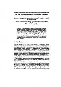
Figure 4.1: Variation of allowable η for filtered white noise

where z is a unit delay. Define

vα = Fα v |Rvα (τ )| τ ∈[1,N ] Rvα (0) P −1 jωk (v ) e supω∈[0,π) N1 N α k k=0 q η2 (α) = 1 N Rvα (0)

η1 (α) = max

Then η1 (α), η2 (α) indicate the minimum permissible values of η for vα ∈ VσN ,η,N and for vα ∈ VσωN ,η,N respectively (with σN2 =

1 N Rvα (0)).

Fig. (4.1) shows plots of η1 (α) (solid) and

η2 (α) (dashed) as α is varied from 0 to 0.9, for a typical zero mean, unit variance random vector v generated by randn command in MATLAB. It is seen that VσωN ,η,N still includes vα for a small value of η, but VσN ,η,N requires rather large values of η even for a modest ‘colouring’ of white noise. Noise sets with low correlation properties are also investigated in relation to robust H2 analysis in [Pag95] and in relation to affinely parameterised approximation problems in [VD], [VD97], [TL95] and [FS99].


4.2.3

27


The estimate Pω0 is given by Pω0

N −1 1 X Yk αN

=

2 αN

=

k=0 N −1 X

if ω0 = 0

Yk ejω0 k

otherwise

(4.12)

k=0

Remark 4.1 The implementation of this algorithm suggested is actually identical to the ‘classical’ method available in literature ([Lju99], ch. 6). The difference is that, here the algorithm is justified purely from a worst case perspective, rather than from a statistical perspective.

4.2.4

Upper Bounds on Identification Errors

Theorem 4.2 For the algorithm stated above,

s

σN e1 (AN : ω0 , γ, ρ, η, σN , α, N ) ≤ L(γ, ρ, N, ω0 ) + β α

1−η 1 ω0 N η+ + 1− sin N N 2 (4.13)

e2 (AN : ω0 , γ, ρ, η, σN , α, N ) ≤ L(γ, ρ, N, ω0 ) + β η

σN α

(4.14)

where L(γ, ρ, N, ω0 ) = =

γρ(1 − ρ−N ) if ω0 = 0 N (ρ − 1)2 γρ(1 − ρ−N ) 1 1 + N (ρ − 1) ρ − 1 sin ω0

(4.15) otherwise

(4.16) (4.17)

and

β = 1

if ω0 = 0

= 2

otherwise

Proof : See Appendix A. Remark 4.2 For a priori information v ∈ VσωN ,η,N , robust convergence follows since γ, ρ, η, σN , α are arbitrary. For a priori information v ∈ VσN ,η,N , robust convergence with respect to η requires an additional condition on N : N=

2π m, for some integer ω0

m

(4.18)

4.3 Identification of Multiple Frequency Response Samples

28

that is, the data consists of an integer number of cycles of input. This is always possible due to condition (4.5) on ω0 . The factor (N sin ω0 ) in L(γ, ρ, N, ω0 ) may appear surprising at first. We show here that this factor basically relates to the integer number of sinusoid input cycles completed by data. Let 0 < ω0 =

2π r

0 and li ≥ 0.

Find : N × [0, π)m × Rm 7→ Cm which maps the experimental data into a An algorithm Am N : R

m−vector of point frequency response estimates Pω = [ Pω1 , Pω2 , . . . , Pωm ]T , Pωi := (Am N (Y, W, α)) (i) such that the worst case errors defined by e1 (Am N : W, γ, ρ, η, σN , α, N ) = sup i∈[1,m]

e2 (Am N : W, γ, ρ, η, σN , α, N ) = sup i∈[1,m]

sup

|Pωi − P (ejωi )|

P ∈BH∞,ρ (γ)

v ∈ VσN ,η,N

sup

|Pωi − P (ejωi )|

P ∈BH∞,ρ (γ) v ∈ Vσω ,η,N N

converge as lim

lim ep (Am = 0 p = 1, 2 N : W, γ, ρ, η, σN , α, N )

σN →0 N →∞

lim lim ep (Am = 0 p = 1, 2 N : W, γ, ρ, η, σN , α, N )

η→0 N →∞

(4.22)

Further, find an upper bound on ep (Am N : W, γ, ρ, η, σN , α, N ) as a function of γ, ρ, η, σN , α, N and W .

4.3.2


The estimates Pωi are given by Pωi = =

N −1 1 X Yk αi N

2 αi N

0 N −1 X 0

if ωi = 0

Yk ejωi k

otherwise

(4.23)

4.4 Probabilistic Bounds in Bounded White noise

4.3.3

30

Bound on Worst Case Error

Theorem 4.3 For the algorithm stated above, e1 (Am N : W, γ, ρ, η, σN , α, N ) ≤ L(γ, ρ, N, α, W ) + s 2σN ωi N 1−η 1 η+ + 1− max sin αmin N N i∈[1,m] 2 e2 (Am N : W, γ, ρ, η, σN , α, N ) ≤ L(γ, ρ, N, α, W ) + 2 Here

γρ(1 − ρ−N ) L(γ, ρ, N, α, W ) = N (ρ − 1)

ησN αmin

1 + (m − 1)ψα φW ρ−1

(4.24)

(4.25)

where αmin = mini∈[1,m] αi and ψ : Rm 7→ R, φ : Rm (π) 7→ R are functions defined by αi i,j∈[1,m] αj 

ψα := max

φW := max  i,j∈[1,m] ωi ≥ωj

(4.26) 

sin

1 ωi +ωj 2

+

sin

1 ωi −ωj 2



(4.27)

Proof : See Appendix A. Intuitively, the task of separating information about the system response at different frequencies from a single experiment seems a difficult task if the frequencies are closely spaced. The definition of φW captures this fact; the error bound deteriorates as the difference max{ωi − ωj , (π − ωi ) − ωj } becomes smaller.

4.4

Probabilistic Bounds in Bounded White noise

Instead of using deterministic noise sets, one may also use probabilistic noise description, along-with deterministic assumptions on the true plant. This leads to probabilistic bounds, or confidence intervals. The following result gives one such confidence interval: Lemma 4.1 Suppose the true plant P ∈ BH∞,ρ (γ) and let the measurement noise be zero mean, white stochastic process bounded in [−K, K]. Given the same a posteriori information as in section 4.2.1 and given any confidence level 0 < ζ < 1, the estimate Pω0 as defined in (4.12) satisfies P

|Pω0

4K − P (ejω0 )| ≤ L(γ, ρ, N, ω0 ) + √ α N

Here L(γ, ρ, N, ω0 ) is as defined in the equation (4.15).

1 ! 2 4 >ζ log 1−ζ

(4.28)

4.4 Probabilistic Bounds in Bounded White noise

31

Proof : See Appendix A. If Pω0 := AN (Y, ω0 , α) is considered as a sequence of random variables indexed by N , it follows from the proof of (4.28) and from the definition of L(γ, ρ, N, ω0 ) that P |Pω0 − P (ejω0 )| >

N →∞ −→ 0, ∀

In other words, Pω0 tends to P (ejω0 ) in probability ([Pap91], chapter 8). Besides this nice convergence result and its non-asymptotic nature, (4.28) is still somewhat pessimistic from a practical point of view. To see this, suppose, we want a confidence level ζ = 0.99 and want to restrict noise term in the error bound to 0.1. Further, suppose K α = 1. The constraint n o 1 2 4 √4 log 1−0.99 ≤ 0.1 yields N ≥ 9587 as a lower bound on the number of samples N required to achieve this. Experiment durations as long as this may be unacceptable in many practical cases.

Chapter 5

New Untuned Algorithms for Worst Case Identification 5.1

Introduction

Worst case identification has attracted a lot of attention since its definitive formulation in [HJN91]. There are two objectives in this problem formulation • To map the experimental frequency response data into a stable plant transfer function via a ‘convergent’ algorithm. An algorithm is said to be convergent if the worst case identification error (with respect to noise and the unknown system) tends to zero as the number of data points tends to infinity and the (deterministic) noise tends to zero. • To provide bounds on the worst case identification error. This problem can be approached in two different ways, leading to untuned and tuned algorithms. Both approaches assume that the true, unknown plant belongs to a certain subset Ψ of the set of stable systems and that the additive noise corrupting the measurement belongs to a certain norm bounded set Ξ. Suitable choices of Ψ and Ξ enable us to derive bounds on the worst case identification error. The identification algorithm is said to be untuned if it is independent of the definitions of Ψ and Ξ; and is said to be tuned otherwise. Examples of algorithms of the the former type may be found in [HJN91], [GK92], [M¨91] and [MP92]; while the later type is investigated in [CNF95], [GLZ96]. An extension of the tuned algorithms to the multivariable case is studied in [CFN96]. Tuned algorithms may give a better result if the plant and the noise 32

5.1 Introduction

33

conform to the assumptions about them, but may fail to give any sensible result at all if the assumptions are wrong. Conventionally, the worst case identification problem is formulated as follows. Assumptions : • The plant P (z) whose transfer function is to be identified is a stable, LSI, SISO discrete time system. Further, P (z) ∈ BH∞,ρ1 (γ1 ). • Noise corrupting measurement belongs to Bl∞ (). Here, the noise bound ∈ [0, ∞), the lower bound on stability margin ρ1 ∈ (1, ∞) and the upper bound on gain γ1 ∈ [0, ∞) are assumed to be known constants. A posteriori Information : A vector of uniformly spaced noisy frequency response samples h Pω = Pω1 where ωi =

2π(i−1) , m

iT Pω2

...

,

Pωm

Pωi = P (ejωi ) + vi

i = 1, 2, . . . , m.

Find : An algorithm Am : Cm 7→ H∞ such that the worst case error defined by e(Am : ρ1 , γ1 , , m) =

sup

kAm (Pω ) − P k∞

P ∈ BH∞,ρ1 (γ1 )

v ∈ Bl∞ ()

converges as lim

m→∞,→0

e(Am : ρ1 , γ1 , , m) = 0

In addition, derive explicit bounds on the above error.

(5.1)

1

Existing untuned algorithms rely on a two step procedure: • Let

m−1 2iπ 1 X P˜m (k) = Pωi e−jk( m ) k = 1, 2, . . . , m m i=0

be the inverse Discrete Fourier Transform Coefficients. Define an L∞ approximation by Pˆ1 =

m X

wm,k P˜m (k)z k

k=−m

Here wm,k is a smoothing function. 1

Note that Am (Pω ) depends on the true plant P and noise v through the relation Pωi = P (ejωi ) + vi .

5.1 Introduction

34

• Solve Nehari’s problem to determine a stable plant nearest to Pˆ1 : Pˆ = arg min kf − Pˆ1 k∞ f ∈H∞

Different untuned algorithms differ in the smoothing or window functions wm,k used in the first step. An example of smoothing function is the triangular window wm,k =

1− 0

|k| m

−m ≤ k ≤ m otherwise

The Nehari approximation step makes the overall scheme nonlinear in a posteriori data. The convergence property of an untuned algorithm is said to be robust if (5.1) holds for every triplet (ρ1 , γ1 , ) ∈ [1, ∞) × [0, ∞) × [0, ∞). Partington [Par92] has shown that it is impossible to construct a linear, robustly convergent algorithm. Since kPˆ − P k∞ ≤ kPˆ1 − P k∞ + kPˆ − Pˆ1 k∞ ≤ 2kPˆ1 − P k∞ , robust convergence can be ensured by a proper choice of window function in the first step. [GK92] gives sufficient conditions on a window function for the algorithm to be robustly convergent. Existing untuned, convergent algorithms seem to suffer from following disadvantages • The class of transfer function models to which the identified model will belong can not be selected a priori. • Uniform frequency spacing is necessary. If nonuniform spacing is used, it needs to be interpolated into uniformly spaced samples to use existing results [AGK92]. • It is not clear how to obtain the a priori information (γ, ρ) necessary to compute the worst case error bound. Moreover, this bound may be conservative, and may not give a true indication of how good - or how poor - the model is. Provided the Nyquist plot of the model is sufficiently smooth and under reasonable (qualitative) assumptions that – the Nyquist plot of the true plant is also smooth and – the measurement noise during point frequency response identification does not have a periodic component, the worst case fit maxi |Pωi − Am (Pω )(i)| over a sufficiently dense grid of measurement frequencies {ωi } is, at least, a good indication of the ‘true’ distance between the plant and the model, rather than the bound on the worst case error. However, most of the existing algorithms do not offer any direct control over the worst case fit maxi |Pωi − Am (Pω )(i)|.

5.2 Identification using Pick interpolation

35

A notable exception which overcomes most of the above anomalies is the finite impulse response approximation algorithm by Mäkil¨ a and Partington [MP92]. More will be said about the algorithm in [MP92] in chapter 6. Here, an alternative untuned algorithm to obtain rational models from a specific subset of H∞ is suggested. It will be motivated by illustrating the shortcomings of direct interpolation of the given frequency response samples using Pick’s theorem.

5.2

Identification using Pick interpolation

First we state Pick’s interpolation theorem [KT85]. Pick’s Theorem : Let ai ∈ D and bi ∈ D, i = 1, 2, . . . , n be two sets of complex numbers. ∃ an analytic function fˆ ∈ H∞ , fˆ : D 7→ D

(5.2)

fˆ(ai ) = bi , i = 1, 2, . . . , m

(5.3)

such that

if and only if the Pick matrix defined by " # 1 − bi b∗j P = , i, j = 1, 2, . . . , m 1 − ai a∗j is nonnegative definite. Further, if the Pick matrix is nonnegative definite, ∃ a rational function fˆ of degree at most m which satisfies conditions (5.2) and (5.3). To apply Pick’s theorem to our present problem, the following corollary is used: Corollary 5.1 Let Pωi and ωi i = 1, 2, . . . , m be two sets of complex numbers with ωi ∈ ∂D. Let ρ2 ∈ R, ρ2 > 1 be a given constant. Then there exists a function Pˆ (z) analytic and bounded in Dρ2 such that Pˆ (ejωi ) = Pωi . Proof : If Pωi = 0 ∀ i ∈ [1, m], then Pˆ (z) = 0 is the required function. Suppose instead, at least one Pωi is nonzero. Let zi =

ejωi ρ2 .

Consider matrix

ˆ = E − α2 F, α ∈ C Q where

"

# 1 E= , 1 − zi zj∗

" F =

Pωi Pω∗j 1 − zi zj∗

# i, j = 1, 2, . . . , m

(5.4)

5.3 Alternate Problem Formulation

36

Let λmax be the largest eigen value of E −1 F . As shown in [KT85], for any α ≤ αmax =

√ 1 , λmax

there exists a rational analytic function Pˆα : D 7→ D such that Pˆα (zi ) = αPωi . A solution to the original interpolation problem is then given by 1 z Pˆ (z) = Pˆα ( ) ∈ H∞ α ρ2

(5.5)

Implementation details of Pick interpolation procedure may be found in ([DFT92], chapter 9). As m → ∞, however, αmax may become arbitrarily small, making kPˆ k∞,ρ2 arbitrarily large. It seems a better way is to find points qi ∈ C such that • |qi − Pωi | is ‘small’; • An analytic function belonging to a norm bounded subset of H∞ interpolates the qi0 s. This idea motivates an alternate problem formulation for worst case identification.

5.3

Alternate Problem Formulation

Assumptions : Identical to those in section 5.1. A posteriori Information : A vector of (not necessarily uniformly spaced) noisy frequency response samples Pω = [Pω1 Pω2 . . . Pωm ]T , Pωi = P (ejωi ) + vi

(5.6)

where ωi ∈ [0, π), i = 1, 2, . . . , m. Also given is a corresponding vector of (angular) frequencies W = [ω1 ω2 . . . ωm ]T

(5.7)

δ = maxi |ωi+1 − ωi | is the maximum separation between adjacent angular frequencies. Let [0, π)m be as defined in (4.20). Given user chosen parameters ρ2 > 1, γ2 > 0, Find an algorithm Aδ1 : C m × [0, π)m 7→ BH∞,ρ2 (γ2 ) such that max |Pˆ (ejωi ) − Pωi | i

is minimised, where Pˆ (z) = Aδ1 (Pω , W ). Further, find an upper bound on the worst case error defined by e (Aδ1 : ρ1 , γ1 , ρ2 , γ2 , , δ) :=

sup P ∈ BH∞,ρ1 (γ1 ), v ∈ Bl∞ ()

k Aδ1 (Pω , W ) − P k∞

(5.8)


37

Remark 5.1 Actually, it is possible - and indeed, more meaningful - to use noise sets defined in chapter 4 in place of Bl∞ (). This will complicate notation, however, as the error definition and convergence will involve both the length of each experiment and the number of experiments (i.e. the number of frequency response samples). Hence we keep using Bl∞ () as the noise set; keeping in mind that may actually be replaced by (4.13) or (4.14).

5.3.1

New Identification Algorithm

As stated above, our aim is to solve min

f ∈BH∞,ρ2 (γ2 )

max |f (ejωi ) − Pωi |

(5.9)

i

The steps to solve the above problem are enumerated below. 1. Find x ˆ, w ˆ1 , w ˆ2 , . . . , w ˆn which solve the following minimisation problem min

λ

(5.10)

 ≥ 0

(5.11)

x∈R, w1 ,w2 ,... ,wm ∈C

subject to LMI constraints 

λx wi∗

diag 

wi 



λx

1

xPω∗i + wi∗

xPωi + wi

1

diag 





E −1

diag (xPω∗i

diag(xPωi + wi )

+

  ≥ 0

wi∗ )

(5.12)

 ≥0

(5.13)

E

and x ≥ γ2−1 Here

 E=

(5.14)

 1 1−

ej(ωi −ωj ) ρ22

 i, j = 1, 2, . . . , n

and diag (xi ) denotes a diagonal matrix with xi , i = 1, 2, . . . , m along its diagonal.


38

2. Find a rational analytic function f : D 7→ D of degree ≤ 2m such that jωi −jωi e e f =x ˆPωi + w =x ˆPω∗i + w î , f î∗ , i = 1, 2, . . . , m ρ2 ρ2

(5.15)

As will be seen in the proof of theorem 5.1, the existence of the interpolant f is ensured by (5.11) - (5.14). Complex conjugate interpolation data is required to obtain a real rational transfer function. If f (z) which satisfies (5.15) is such that f (z) = f1 (z)+jf2 (z) jω where f1 , f2 are real rational functions, f1 (z) also obeys f1 eρ2 i = x ˆPωi + w î , i = 1, 2, . . . , m [DFT92]. 3. The identified transfer function model is then given by z Pˆ (z) = x ˆ−1 f1 ( ) ρ2

(5.16)

Note that solving the above problem requires no assumptions as to how (ρ1 , γ1 ) and (ρ2 , γ2 ) are related, i. e. the a priori information is not in-built in the algorithm. The user is free to choose (ρ2 , γ2 ) so as to obtain a desired compromise between a good worst case error fit and an acceptable smoothness for Pˆ (z) (since kPˆ 0 k∞ ≤

γ2 ρ2 −1 ).

We now prove that the above procedure indeed gives the required transfer function. Theorem 5.1 When Pˆ (z) is obtained as outlined above, max |Pˆ (ejωi ) − Pωi | =

min

max |f (ejωi ) − Pωi |

f ∈BH∞,ρ2 (γ2 ) i∈[1,m]

i∈[1,m]

(5.17)

Proof : Let P˜ ∈ BH∞,ρ2 (γ2 ) such that sup |P˜ (z)| ≤ x−1

(5.18)

Let P˜ (ejωi ) = Pωi + w ˜i , i = 1, 2, . . . , m

(5.19)

z ∈ Dρ 2

for some x ∈ R .

Then we seek to minimise maxi |w ˜i |. Define

fˆ(z) = xP˜ (ρ2 z)

(5.20)

and wi = x w ˜i . Then equations (5.20), (5.18) ⇔ supz∈D |fˆ(z)| ≤ 1. Also, P˜ analytic in Dρ2 ⇔ fˆ(z) is analytic in D. Multiplying both sides of (5.19) by x and using (5.18), xPωi + wi ∈ D

(5.21)


39

Also, using definition of fˆ(z), jωi e ˆ f = xPωi + wi ρ2

(5.22)

It follows that the Pick matrix corresponding to the interpolation pairs

ejωi ρ2 ,

xPωi + wi

must be nonnegative definite, i. e. Q = E − diag(xPωi + wi ) E diag(xPω∗i + wi∗ ) ≥ 0

(5.23)

Inequality (5.12) is equivalent to (5.21), which can be verified using (2.12). Inequality (5.13) is equivalent to (5.23). Inequality (5.14) follows from (5.18) and from the fact that P˜ ∈ BH∞,ρ2 (γ2 ). Finally, max |w ˜i | = max x−1 |wi |

i∈[1,m]

i∈[1,m]

Since x > 0, the right hand side can be minimised by solving min λ subject to max (x2 λ2 − |wi |2 ) ≥ 0 i∈[1,m]

(5.24)

This is achieved by minimising λ subject to (5.11), the equivalence again follows from (2.12).

Thus we have formulated our identification problem as a convex optimisation problem. For any allowable choice of (γ2 , ρ2 ), consider a choice of decision variables x = γ2−1 + q, q ∈ (0, ∞),

wi = −xPωi ∀ i ∈ [1, m]. This corresponds to a solution Pˆ (z) = 0.

We deduce two important properties of our problem formulation from this solution: • The above solution is feasible for any choice of pair (ρ2 , γ2 ) such that ρ2 ∈ (1, ∞), γ2 ∈ (0, ∞). Thus the optimisation problem has a nonempty feasible solution set for all allowable γ2 , ρ2 . • This solution remains feasible if the inequalities in (5.11) - (5.14) are replaced by strict inequalities, i.e. the problem is strictly feasible [BGFB94].2 For a strictly feasible problem, the infimum obtained by solving the problem with non-strict inequalities is same as the one obtained by solving the problem with strict inequalities [BGFB94]. The strict inequalities problem is tractable by easily available and efficient commercial software, without the added complexity of reducing non-strict LMIs to strict LMIs. 2

The only nontrivial step in proving this is to prove that E is positive definite. This is proved using Pick’s

theorem in [CNF95].


5.3.2

40

Worst Case Error Bound

We use a result from [HJN91] which gives a bound on infinity norm on the worst case slope of an exponentially stable system: Fact 5.1 Let f ∈ BH∞,ρ (γ). Then k f (k) k∞ ≤

γk! (ρ − 1)k

dk f (z) . dz k

where f (k) =

Theorem 5.2 Let Pˆ (z) = Aδ1 (Pω , W ). Then δ γ1 γ2 e(Aδ1 : ρ1 , γ1 , ρ2 , γ2 , , δ) ≤ + + λ + ρ1 − 1 ρ2 − 1 2 where

(5.25)

λ = max |Pˆ (ejωi ) − Pωi | i∈[1,m]

Proof : Consider any point ω ∗ ∈ [ωi , ωi+1 ). Applying triangle inequality to the error at this frequency ∗ ∗ ∗ |Pˆ (ejω ) − P (ejω )| ≤ |Pˆ (ejω ) − Pˆ (ejωi )| + |Pˆ (ejωi ) − Pωi | ∗

+ |Pωi − P (ejωi)| + |P (ejωi ) − P (ejω )| ≤ kPˆ 0 k∞ where f 0 (z) :=

df dz .

Similarly, kPˆ k∞ ≤

5.3.3

(5.26)

From fact 5.1, kP 0 k∞ ≤

0

δ δ + λ + + kP 0 k∞ 2 2

γ2 ρ2 −1 .

kP k∞,ρ1 γ1 ≤ ρ1 − 1 ρ1 − 1

Substituting these values in (5.26) gives the result.

Asymptotic Behaviour of Worst Case Error

Let δ = mini |wi+1 − wi | be the minimum angular frequency separation. Define einf := 1 limδ→0 lim→0 e(Aδ1 : ρ1 , γ1 , ρ2 , γ2 , , δ) where limδ→0 is taken such that the ratio

δ δ

is always

bounded. Lemma 5.1 einf 1

≤ γ1 always

(5.27)

= 0 if BH∞,ρ1 (γ1 ) ⊆ BH∞,ρ2 (γ2 )

(5.28)

5.4 Achieving Robust Convergence

41

Proof : First, let BH∞,ρ1 (γ1 ) ⊆ BH∞,ρ2 (γ2 ). Since P ∈ BH∞,ρ1 (γ1 ) ⊆ BH∞,ρ2 (γ2 ), λ=

min

F ∈ BH∞,ρ2 (γ2 )

max |F (ejωi ) − Pωi | ≤ max |P (ejωi ) − Pωi | ≤ i

i

Substituting in (5.25) and taking appropriate limits leads to (5.28).

(5.29)

If BH∞,ρ1 (γ1 ) 6⊆

BH∞,ρ2 (γ2 ), then the trivial solution Pˆ (z) = 0 gives einf ≤ lim lim max |Pωi | ≤ γ1 1 δ→0 →0

i

Suppose BH∞,ρ2 (γ2 ) reflects our knowledge about the true plant set BH∞,ρ1 (γ1 ). Then the algorithm converges if our a priori information is correct. This resembles convergence of tuned algorithms. Even if the a priori information is incorrect, however, the proposed algorithm retains its bounded error property.

5.4

Achieving Robust Convergence

A part of the bound on the worst case error is fixed by a priori information, γ1 , ρ1 and . The remaining part depending on a posteriori information is er (Aδ1 : ρ2 , γ2 , δ) = kPˆ 0 k∞,ρ2

δ +λ 2

where λ = maxi |Pˆ (ejωi )−Pωi |, Pˆ (z) = Aδ1 (Pω , W ) and kPˆ 0 k∞ ≤

(5.30)

kPˆ k∞,ρ2 ρ2 −1

from [HJN91].

Instead of minimising worst case absolute distance, consider the following problem: Given the same a priori and a posteriori information as before and a user chosen lower bound on stability margin ρ2 , Find an algorithm Aδ2 : C m × [0, π)m 7→ H∞,ρ2 such that

! kPˆ k∞,ρ2 δ jωi ˆ + max |P (e ) − Pωi | i ρ2 − 1 2

(5.31)

is minimised, where Pˆ (z) = Aδ2 (Pω , W ). The procedure to solve the above problem is given below. 1. Solve min

x∈R, w1 ,w2 ,... ,wn ∈C

subject to LMI constraints



diag 

λx − k

wi∗

λ 

 ≥ 0 λx − k and constraints given by (5.12), (5.13). Here k = ρ21−1 δ2 . wi

(5.32)

(5.33)

5.4 Achieving Robust Convergence

42

Steps 2 and 3 are identical to those in in section 5.3.1. By using arguments nearly identical to those used in case of Aδ1 , it can be shown that the above procedure solves (5.31). Further, define the worst case error as before e2 (Aδ2 : ρ1 , γ1 , ρ2 , , δ) :=

sup P ∈BH∞,ρ1 (γ1 ), v∈Bl∞ ()

k Aδ2 (Pω , W ) − P k∞

(5.34)

with the asymptotic value defined as einf := limδ→0 lim→0 e(Aδ2 : ρ1 , γ1 , ρ2 , , δ). We have 2 the following result: Lemma 5.2 einf 2

≤ γ1 always

(5.35)

= 0 if ρ2 ≤ ρ1

(5.36)

Proof: similar to the proof of lemma 5.1. Since

kPˆ k∞,ρ2 ρ2 −1

is an upper bound on kPˆ 0 k∞ , the above lemma introduces the idea of trade-

off between the worst case fit achieved and the worst case slope of approximation (which controls the behaviour of the model in-between the measurement samples). This idea will be one of the central themes in chapters 6 and 7. Note that lemma 5.2 is a stronger statement of convergence than lemma 5.1. A natural extension is to go a step further and pose a problem: Given the same a priori and a posteriori information as before, Find an algorithm Aδ3 : C m × [0, π)m 7→ H∞ such that Aδ3 solves min

min

ρ∈(1,∞) Pˆ ∈H∞,ρ

! kPˆ k∞,ρ δ jω + max |Pˆ (e i ) − Pωi | i ρ−1 2

(5.37)

where Pˆ (z) = Aδ3 (Pω , W ). Lemma 5.3 Aδ3 is robustly convergent algorithm. Proof: Defining the worst case error and its asymptotic value as before, the above result follows from lemma 5.2. The outermost minimisation is non-convex in ρ. An approximate solution may be sought for finite data size by solving (5.31) for different values of ρ.

5.5 Simulation Example

5.5

43

Simulation Example

We illustrate the use of the first algorithm proposed here by identifying a discrete transfer function P (z) =

N (z) D(z) ,

with N (z), D(z) given by

N (z) = 2(0.141z 6 + 0.2618z 5 + 0.5229z 4 + 0.1691z 3 + 0.2736z 2 + 0.2674z + 0.042) D(z) = 0.2897z 7 + 0.1111z 6 + 0.0776z 5 + 0.3671z 4 + 0.4575z 3 + 0.2973z 2 + 0.3557z + 1 This transfer function is the same as that used in [GXZ93] to demonstrate a tuned algorithm. It is scaled up by 2 to avoid (5.12) from becoming trivially true. 32 uniformly spaced noisy point frequency response samples were identified by the algorithm described in chapter 4. For each frequency, length of data used for (4.12) is N = 500. Gaussian white noise of variance approximately 10% of 2-norm of ‘clean’ output data is added. Matlab’s LMI control toolbox was used for solving the optimisation problem (5.9) for these frequency response samples. First, the parameters for BH∞,ρ2 (γ2 ) were γ2 = 10 maxi |Pωi |, ρ2 = 1.05. In figures (5.1), the solid line represents the true transfer function and the dashed line represents the frequency response of the identified model. ‘∗’ denotes the frequency response samples Pωi . The effect of spurious poles and zeroes is clearly evident in the model plots. Changing the value of γ2 to upto γ2 = 1.1 maxi |Pωi | does not yield any significant improvement in the ‘smoothness’ of Nyquist plot (or worst case slope).


44

2

True plant model point samples

Magnitude

1.5

1

0.5

0

0.5

1

1.5

2

2.5

3

3.5

frequency

Figure 5.1: Magnitude plots of true plant and identified model

2

1.5

1

0.5

0

−0.5

−1 −1.5

−1

−0.5

0

0.5

1

Figure 5.2: Nyquist plots of true plant and identified model

1.5

Chapter 6

Worst Case Identification using FIR Models 6.1

Introduction

In section 5.4, the idea of obtaining a model that gives the best worst case fit subject to a constraint on its slope (in terms of γ2 , ρ2 ) is introduced. The algorithms in chapter 5 still share one major disadvantage with other worst case methods - the model order is a function of length of data. This restriction is removed in this chapter, obtaining a robustly convergent algorithm which is optimal, in a certain sense, for a finite model order. Further motivation of this work comes from the analysis of the optimal achievable worst case error by Zames et al in [ZLW94] and from a subsequent tuned FIR approximation scheme suggested by Glaum, Lin and Zames [GLZ96]. The Kolmogorov n-width of a subset P ⊂ H∞ , in H∞ is defined by [Pin85] dn (P) = inf sup

inf kx − yk∞

Xn x ∈ P y ∈ Xn

(6.1)

where the left-most infimum is taken over all n-dimensional subspaces of H∞ . Thus dn (P) represents the optimal worst case error one can achieve by approximating a system in P by a linear combination of n basis functions in H∞ . A subspace which actually achieves this error is called an optimal subspace for P. We are interested in two plant sets: P1 (γ, ρ) = BH∞,ρ (γ)

and

P2 (M ) = {f : f ∈ H∞ , k f 0 k∞ ≤ M } 45

(6.2)

6.2 Problem Formulation

where f 0 (z) :=

df dz .

46

For both P1 (γ, ρ) and P2 (M ), an optimal subspace is Sn = span{1, z, . . . , z n−1 }

(6.3)

where span is over the real field. Further, the exact values of n-widths in these cases are [Pin85] dn (P1 (γ, ρ)) = γρ−n , dn (P2 (M )) =

M n

(6.4)

n→∞

Clearly, dn (Pi ) −→ 0, i = 1, 2. Contrary to intuition however, an optimal approximation is not always given by the first n impulse response parameters.

6.2

Problem Formulation

Assumption : The plant transfer function P (z) to be identified is a stable, linear, shift invariant, SISO discrete time system. A priori Information : • P (z) belongs to either of the plant sets Pi , i = 1, 2. • Noise v corrupting measurement belongs to Bl∞ (). Here, ∈ [0, ∞), either M ∈ [0, ∞) or ρ ∈ (1, ∞) and γ ∈ [ 0, ∞) are assumed to be known constants. A posteriori Information : A vector of (not necessarily uniformly spaced) noisy frequency response samples Pω = [Pω1 Pω2 . . . Pωm ]T , Pωi = P (ejωi ) + vi

(6.5)

where ωi ∈ (0, π), i = 1, 2, . . . , m. Also given is a corresponding vector of (angular) frequencies W = [ω1 ω2 . . . ωm ]T

(6.6)

δ = maxi |ωi+1 − ωi | and δ = mini |ωi+1 − ωi | are the maximum and the minimum separation between adjacent angular frequencies respectively. Let [0, π)m be as defined in (4.20). Find : An algorithm Aδ : Cm × [0, π)m 7→ Sn such that the worst case errors defined by ei (Aδ : xi , , n, δ) =

sup P ∈ Pi (xi ),v ∈ Bl∞ ()

k Aδ (Pω , W ) − P k∞

(6.7)

6.3 Identification Algorithm

47

converge as follows lim ei (Aδ : xi , , n, δ) ≤ dn (Pi ) + β

δ→0

lim ei (Aδ : xi , , n, δ) ≤ gi (xi , δ, )

(6.8)

n→∞

where i = 1, 2, x1 = (γ, ρ), x2 = M , and δ → 0 in such a way that

δ δ

remains bounded. gi

are some functions bounded for fixed xi , monotonically increasing in both δ and such that lim→0 limδ→0 g(α, δ, ) = 0. In addition, derive explicit bounds on the above error. An important feature of this formulation is the separation of the error convergence with respect to the increasing model order and that with respect to the increasing number of data points. Existing robustly convergent algorithms rely on model order being some increasing function of the number of data points for the error to go to zero. The proposed algorithm removes this constraint, giving a significantly stronger convergence property.

6.3


Aδ (Pω , W ) ∈ Sn is a solution of the following optimisation problem: minimise λ subject to f ∈ Sn and max | f (e

jωi

max

i∈[1,m]

) − Pωi |, k˜1 k f 0 k∞

0

Li < λ Ri , i = 1, 2

(6.14)

(6.15)

(6.16)

• Let a ˆk , k = 0, 1, . . . , n − 1 be the values of decision variables which minimise λ. Then Aδ (Pω , W ) =

n−1 X

a ˆk z k

k=0

It remains to be shown that the procedure outlined above actually amounts to solving (6.9). P Theorem 6.1 Let Pˆ (z) = n−1 ˆk z k , with a ˆk obtained as above. Then k=0 a jωi 0 jωi 0 ˜ ˜ ˆ ˆ max max |P (e ) − Pωi |, k1 kP k∞ = inf max max | f (e ) − Pωi |, k1 k f k∞ i

f ∈Sn

i

(6.17)

6.4 Convergence and a priori Error Bounds

Proof : Let f (z) =

Pn−1 k=0

49

ak z k . Note that minimising max {| f (ejωi ) − Pωi |, k˜1 k f 0 k∞ }

is same as minimising max {k˜1−1 | f (ejωi ) − Pωi |, k f 0 k∞ }.

From [GA94] and from defini-

tions (6.10), (6.11), the conditions     

AT XA − X B T XA

λ−1 C T

AT XB B T XB

λ−1 C

−1

λ−1 D

λ−1 D −1

    0 correspond to kf 0 k∞ < λ. Also, k˜1−1 | f (ejωi ) − Pωi | < λ is enforced by  diag 

k˜1 λ

Pω∗i − θ T φ∗i

Pωi − φi θ

k˜1 λ

  > 0

(6.19)

Rearranging these LMIs gives (6.16).

Remark 6.1 In [MP92], a closely related problem is solved : minimise λ subject to f ∈ Sn and jωi 0 max max | f (e ) − Pωi |, k1 k f k1 < λ

(6.20)

i∈[1,m]

where k f 0 k1 =

Pn−1 i=0

k|fk |, fk being parameters of f . Solution to this problem also yields

a robustly convergent algorithm. The algorithm presented here has a significantly stronger convergence property. It also generalises nicely to the coprime factor identification case, as will be seen in section 6.6.

6.4

Convergence and a priori Error Bounds

Let ω ∗ ∈ [0, π). For convenience of notation, denote Pˆ (z) = Aδ (Pω , W ) (z). Then by triangle inequality, ∗ ∗ ∗ |Pˆ (ejω ) − P (ejω )| ≤ |Pˆ (ejω ) − Pˆ (ejωi )| + ∗

|Pˆ (ejωi ) − Pωi | + |Pωi − P (ejωi)| + |P (ejωi ) − P (ejω )|

(6.21)

≤ kPˆ 0 k∞ 2δ + λ + + kP 0 k∞ 2δ where λ = |Pωi − Pˆ (ejωi )| and f 0 (z) = δ→0

df dz .

For any P in P1 or in P2 , P 0 ∈ H∞ and

kP 0 k∞ 2δ −→ 0. Hence the convergence result (6.8) holds for Aδ if, for P ∈ Pk , k = 1, 2, the

6.4 Convergence and a priori Error Bounds

50

FIR approximation Pˆ satisfies the following properties: δ 0 jωi ˆ ˆ lim max kP k∞ , max | P (e ) − Pωi | ≤ g(xi , δ, ) < ∞ n→∞ i 2 δ lim max kPˆ 0 k∞ , max | Pˆ (ejωi ) − Pωi | ≤ β + dn (P1 ) ∀ i ∈ [1, m] i 2 δ→0

(6.22) (6.23)

where limδ→0 lim→0 g(xi , δ, ) −→ 0 for fixed xi and β is independent of both data and a priori information. The error bound is derived and the convergence of the algorithm is proved by demonstrating the existence of feasible solution to the optimisation problem (6.9) which have the required convergence properties (6.22) and (6.23). For P ∈ P2 , a feasible solution with the required properties is given by the following result of Glaum et al ( [GLZ96, lemma 3.1]): Lemma 6.1 ([GLZ96]) For a priori information v ∈ Bl∞ (), P ∈ P1 and a posteriori information as in section 6.2, there exists a Pˆ (z) ∈ Sn which satisfies the following constraints: |Pˆ (ejωi ) − Pωi | ≤ + kPˆ 0 k∞ < M +

M Mδ + n 4

(6.24)

2M nδ

(6.25)

where δ > 0 is arbitrary. Using an argument identical to that used for proving the above lemma in [GLZ96] and employing fact 5.1, one can prove the following result for P ∈ P1 : Lemma 6.2 For a priori information v ∈ Bl∞ (), P ∈ P1 and a posteriori information as in section 6.2, there exists a Pˆ (z) ∈ Sn which satisfies the following constraints : |Pˆ (ejωi ) − Pωi | ≤ + γρ−n + kPˆ 0 k∞
0 is arbitrary. Theorem 6.2 lim ei (Aδ : xi , , n, δ) ≤ g(xi , δ, )

n→∞

lim ei (Aδ : xi , , n, δ) ≤ 2 + dn (Pi )

(6.28)

δ→0

where i = 1, 2, x1 = {γ, ρ}, x2 = M and g(·) is such that limδ→0 lim→0 g(xi , δ, ) = 0 for fixed xi .

6.5 Modifications and Extensions

Proof: Let k˜1 = k1 δ

r

51

where 0 < k1 < ∞ and 0 < r < 1 are constants. For P ∈ P2 , it is

clear from lemma 6.1 that

0

r

min max max | f (e ) − Pωi |, k1 k f k∞ δ i∈[1,m] r M 2M Mδ < max + δ + , k1 M + n 4 nδ jωi

f ∈Sn

(6.29)

ζ for an arbitrary δ > 0. Choose δ =

δ n

for an arbitrary ζ, 0 < ζ < r and let

r 2M M Mδ := max + δ + , k1 M + n 4 nδ r−ζ )! ζ ( r 2k1 M δ M M δ = max + , k1 M δ + + n 4 n n1−ζ

λopt

(6.30)

Using (6.21), (6.29) and (6.30), e(Aδ : M, , n, δ) ≤

Also, and

! 1−r δ 1 δ + 1 λopt + M + k1 2 2

(6.31)

r lim λopt = max , k1 M δ

n→∞

lim λopt = + δ→0

M n

(6.32)

The result follows from (6.31) and (6.32). Proof for P ∈ P1 follows similarly using lemma 6.2.

6.5 6.5.1

Modifications and Extensions Obtaining Smooth Approximations

For a fixed n and Pω , k˜1 in (6.9) serves as a trade off between smoothness of the approximation (in terms of kPˆ 0 k∞ ) and the achieved fit to the data. A tighter control over the smoothness of Pˆ (z) may be obtained by using kPˆ 0 k2 or kPˆ 00 k∞ . The following result lends justification to the use of kPˆ 00 k∞ : Lemma 6.3 Let Pˆ ∈ H∞ . Let ωi and ω ∗ be two angular frequencies such that |ωi − ω ∗ | ≤ δ2 . Then 2

∗ δ δ |Pˆ (ejωi ) − Pˆ (ejω )| ≤ |Pˆ 0 (ejωi )| + kPˆ 00 k∞ 2 4

(6.33)


52

Proof : Define f : [0, π] 7→ C, such that f (ω) := Pˆ (ejω ) From ([Rud76], chapter 5), | f (ωi ) − f (ω ∗ )| ≤ where f 0 (ω) =

df dω .

sup ω ∈ [ωi

,ω ∗ ]

| f 0 (ω)||ωi − ω ∗ |

(6.34)

Let the supremum of f 0 (ω) be attained at a frequency ω ˜ . Then us-

ing (6.34), | f (ωi ) − f (ω ∗ )| ≤ | f 0 (˜ ω )||ωi − ω ∗ | = | f 0 (˜ ω ) + f 0 (ωi ) − f 0 (ωi )||ωi − ω ∗ | ≤ | f 0 (˜ ω ) − f 0 (ωi )||ωi − ω ∗ | + | f 0 (ωi )||ωi − ω ∗ | ! δ δ ≤ sup | f 00 (ω)||ωi − ω ˜| + | f 0 (ωi )| 2 2 ω ∈ [ωi ,˜ ω]

(6.35) (6.36)

2

≤

sup | f 00 (ω)|

ω ∈ [0, π]

δ δ + | f 0 (ωi )| 4 2

(6.37)

Note that (6.36) follows from (6.35) by employing (6.34) for f 0 (ω). Now, using chain rule for differentiation gives 0 df dPˆ f (ω) = = dω d(ejω )

jω d(e ) dPˆ dω = d(ejω )

(6.38)

2 ˆ Similarly, | f 00 (ω)| = d(ed jωP)2 . As Pˆ (z) ∈ H∞ , Pˆ 0 (z) ∈ H∞ , Pˆ 00 (z) ∈ H∞ . Therefore | f 0 (ωi )| = |Pˆ 0 (ejωi )| and sup[0,π] | f 00 (ω)| = sup[0,π] |Pˆ 00 (ejω )| = kPˆ 00 k∞ . This completes the proof.

P Let Pˆ (z) = Aδ (Pω , W ) = n−1 ˆk z k . Then the condition k=0 a kPˆ 00 k∞ < λ is affine in the parameters a ˆk of Pˆ (z). It is hence possible to modify (6.9) and pose an LMI problem

minimise λ subject to max max |Pˆ (ejωi ) − P (ejωi )|, k˜1 kPˆ 0 k∞ , k˜2 kPˆ 00 k∞ < λ i

(6.39)


53

where k˜1 , k˜2 are user chosen nonzero weights. One may choose to replace k˜1 kPˆ 0 k∞ by maxi k˜1 |Pˆ 0 (ejωi )| . As k˜1 is a free parameter, both representations are equally good. The former leads to a higher number of decision variables, the latter, in general, to a higher number of LMI constraints. Lemma 6.4 For a priori information v ∈ Bl∞ (), P ∈ P1 (γ, ρ) and a posteriori information as in section 6.2, there exists Pˆ (z) ∈ Sn such that

|Pˆ (ejωi ) − Pωi |, k˜1 kPˆ 0 k∞ , k˜2 kPˆ 00 k∞ γ 2γ ˜ ˜ ≤ max + αdn (P1 ), k1 , k2 (ρ − 1) (ρ − 1)2

max

where α =

ρ ρ−1 .

Proof : Let P (z) =

P∞

i=0 pk z

k

Pn−1 k and choose Pˆ (z) = i=0 pk z . The result follows using

fact 5.1 and using |Pˆ (ejωi ) − Pωi | ≤ + |Pˆ (ejωi ) − P (ejωi )|

(6.40)

Using (6.22)- (6.23) and the above lemma, it is seen that (6.39) only slightly weakens the convergence properties (6.8) for P ∈ P1 (i.e. the worst case error is within a constant factor α). Similarly, kPˆ 0 k2 may also be incorporated in the min-max problem (6.39) as an additional P smoothness constraint. With Pˆ (z) = n−1 ak z k and C, D as defined in (6.11), k=0   λ 0 CT      0 λ D  > 0 ⇔ kPˆ 0 k2 < λ   C D λ

6.5.2

Using fixed pole structures

Let S(z) =

Pl−1

k=0 sk z

k

be a user chosen polynomial of degree r − 1 such that S −1 ∈ H∞ .

S(z) may represent the user’s knowledge about pole locations, based on elementary tests like step response. Define a function dˆn by dˆn = dn (P1 ) n > 0 = γ

n≤0

(6.41)

Consider the following problem : Given a priori information v ∈ Bl∞ (), P ∈ P1 (γ, ρ), the same a posteriori information as in


54

section 6.2 and additionally a user chosen polynomial S(z) of degree l − 1, Find : An algorithm Aδ : Cm × [0, π)m 7→ Sn such that, for IIR transfer function Pˆ (z) = Aδ (Pω ,W ) , S(z)

the worst case error defined by e1 (Aδ : γ, ρ, , n, δ) =

sup P ∈P1 (γ, ρ),v∈Bl∞ ()

kPˆ − P k∞ ,

(6.42)

converges as lim e1 (Aδ : γ, ρ, , n, δ) ≤ αdˆn−l + β

(6.43)

δ→0

for some constants α, β independent of n and δ. P k Solution : Let Q(z) = n−1 k=0 (Aδ (Pω , W ))(k)z . Then 0 − QS 0 SQ 0 Pˆ (z) = (z) S2

(6.44)

The above expression is affine in the parameters of Q(z). Consequently, the following problem may be written as an affine problem in the parameters of Q(z), minimise λ subject to max

max |Pˆ (ejωi ) − Pωi |, k˜1 kPˆ 0 k∞

i

0, ∀ejω ∈ ∂D. Since the cost function is continuous in f , a small δf will cause only a small increase in cost.

7.4

Approximation in the L2 -gap

An iterative procedure for approximation in the L2 -gap is given below. SISO case is discussed here for ease of notation. Let Sn and S1,2 be defined as in (6.3) and (6.49) respectively. Given : A vector of frequency response samples Pω defined as in (7.12). ˆ 0 = 1. Initialisation : Set k = 1, Q Step A : Solve min

fk ∈S1,2

ˆ k−1 )(ejωi ), αkf 0 k∞ max σ (F − fk Q k i

(7.18)

where α is a user chosen constant, F (ejωi ) is obtained from P0 (ejωi ) using (7.17) and fk0 = dfk dz .

ˆ k−1 )(ejωi ) ≤ λ This problem is similar to (6.53). Both the constraints σ (F − fk Q

7.4 Approximation in the L2 -gap

67

and αkfk0 k∞ < λ may be written as affine constraints in the parameters of fk , the latter using (6.18) and suitable definitions of matrices A, B, C, D. Thus, (7.18) may be written as an LMI optimisation problem. Let fˆk be the solution to (7.18). Step B : Solve min

max σ (F − fˆk Qk )(ejωi )

Qk (ejωi ) i∈[1,m]

(7.19)

This step is an unconstrained linear least squares problem, and has a closed form solution: jωi ˆ∗ jωi ˆ k (ejωi ) = fk (e )F (e ) Q fˆk∗ (ejωi )fˆk (ejωi )

(7.20)

ˆ k )(ejωi ) is less than a specified tolerance, stop; otherwise set k := k + 1 If maxi σ(F − fˆk Q and go back to step A. If fˆk∗ fˆk (ejωi ) = 0 for some i ∈ [1, m], we can replace fˆ in (7.20) by fˆk + δfˆk for a small perturbation δfˆk , such that (fˆk + δfˆk )∗ (fˆk + δfˆk ) 6= 0. As the cost function is continuous in fˆk , a small perturbation in fˆk results in a small increase in cost. This, of course, is of theoretical interest; yielding fˆk∗ fˆk (ejωi ) = 0 exactly is a situation rather unlikely to occur in practice. Suppose, α is sufficiently small so that the solution of (7.18) is the same as the solution ˆ k−1 )(ejωi ). of minfk ∈S1,2 maxi σ (F − fk Q

2

ˆ l )(ejωi ). Thus vk,k−1 Define vk,l := maxi (F − fˆk Q

and vk,k give the achieved cost at steps A and B respectively at kth iteration. A particularly attractive property of the above procedure is that the achieved cost in our approximation improves with each iteration. Lemma 7.3 For k ≥ 1, vk,k ≤ vk,k−1 ≤ vk−1,k−1 Proof : Consider step A of kth iteration. Since fˆk−1 is a feasible solution for (7.18), we have ˆ k−1 is a feasible solution for (7.19), vk,k ≤ vk,k−1 . vk,k−1 ≤ vk−1,k−1 . Similarly, as Q Further, a local optimality-like property may be proven for this procedure. Define wk,j := ˆ j )(ejωi ). Let fˆk = fˆk−1 + λ∆, where λ ∈ R and ∆ ∈ S1,2 , k∆k∞ = 1. The following (F − fˆk Q result is based on a similar result in [VM97]. Lemma 7.4 At any point ejωi ,

d d ∗ ∗ = {wk,k wk,k } {wk,k−1 wk,k−1 } dλ dλ λ=0 λ=0

2

(7.21)

In a number of simulation experiments, this assumption is seen to hold for any α < 1, with a sensible

choice of n1 and n2 ..

7.5 Satisfying the Winding Number Constraint

68

∗ fˆ = 0. This gives Proof : From (7.20), wk,k k

d ∗ ˆ k ) + (−∆Q ˆ k )∗ wk,k (−∆Q {w∗ w } = wk,k dλ k,k k,k d ∗ ˆ k−1 ) + (−∆Q ˆ k−1 )∗ wk,k−1 w } = wk,k−1 (−∆Q {w∗ dλ k,k−1 k,k−1

(7.22) (7.23)

The right hand sides of (7.22), (7.23) are equal at λ = 0. This means that if there is a descent direction for minimising σ(F − fk Qk ) simultaneously ˆ k−1 ), then usually, there also exists a descent direction at over (fk , Qk ) at a point (fˆk−1 , Q ˆ k−1 ) over fk alone. ˆ k−1 ) for minimising σ(F − fk Q (fˆk−1 , Q

7.5

Satisfying the Winding Number Constraint

−1 Let P0 represent the true plant. Let P1 = f1,k f2,k , where fˆk = [f1,k f2,k ]T is a solution

to (7.18) at kth iteration. Then the above procedure ensures that maxi κ(P1 , P0 )(ejωi ) < vk,k , but it doesn’t guarantee that I(P1 , P0 ) = 0. This means that P1 may not be stabilised by a controller C, given that C stabilises P0 . Suppose, a controller C which stabilises the true plant P0 results in η (H(P1 , C)) = k and bL2 (P1 , C) = α for a model P1 . From lemma 7.1, if another model P2 satisfies I(P2 , P1 ) ≤ −k and δL2 (P1 , P2 ) < α, then η (H(P2 , C)) = 0. A method for finding P2 which guarantees I(P2 , P1 ) ≤ −k is outlined in the next theorem. Theorem 7.1 Given P1 and γ < 1, the following are equivalent. (i). ∃ P2 : I(P2 , P1 ) ≤ −k and δL2 (P1 , P2 ) < γ q (ii). γ > 1 − σk2 (HG1 ) where σk (HG ) is the kth largest singular value of Hankel operator HG . When the condition (ii) is satisfied, such a P2 may be constructed as P2 = {F ac(X)}∗ where X = [x1 x2 ]T satisfies x−1 ∈ R, X ∈ H∞(−),n−k and k G3 − X k∞ < γ. Here G3 is the 2 normalised right graph symbol for P3 := P1∗ , deg(P1 ) = n and H∞(−),n−k denotes the space of functions analytic outside the unit disk except for at most n − k stable poles. Proof : See Appendix B. As illustrated in the proof of this result, one can construct a P2 which solves inf

P2 ∈R

I(P2 ,P1 )≤−k

δL2 (P1 , P2 )

(7.24)


69

Then by triangle inequality, max κ(P0 , P2 )(ejωi ) ≤ vk,k + δL2 (P1 , P2 )

(7.25)

i

Also, from (7.8), η (H(P2 , C)) = 0 provided bL2 (P1 , C) > δL2 (P1 , P2 ). Since C stabilises P0 , again applying (7.8) for P2 , P0 , C gives I(P2 , P0 ) = 0

(7.26)

provided bL2 (P2 , C) > δL2 (P0 , P2 ). δL2 (P0 , P2 ), in turn, may be approximated by maxi κ(P0 , P2 )(ejωi ). If a ‘good’ chordal distance fit is obtained over a sensible grid of frequencies, this condition is easy to satisfy; as the simulation example in section 7.6 demonstrates. Finally (7.25), (7.26) combine to give δW (P0 , P2 ) ≤ vk,k + δL2 (P1 , P2 ) If both P0 and P1 are stable (i.e. stabilised by C = 0), I(P1 , P0 ) = 0 provided bL2 (P1 , 0) > δL2 (P1 , P0 ). This is a very simple condition to check approximately, and does not require knowledge of any other controller. If the plant is unstable, a stabilising controller is needed to build a model P2 . This is a reasonable requirement; a controller would be needed to collect any operational data anyway. A new, related algorithm for identification of normalised coprime factors appears in [Gu99]. This algorithm is based on discrete Fourier Analysis and is robustly convergent. On the other hand, it relies on uniform frequency spacing and does not cater for the important winding number correction.

7.6

Simulation Example

Consider a continuous time plant P (s) =

1.875s2 + 18.75s + 48.75 s4 + 6.1s3 + 16.4845s2 + 38.431s + 60.197

This plant has two pairs of lightly damped resonant poles and a pair of resonant zeroes. It was mapped to z-plane by Tustin transformation, with a sampling period 0.5 sec. 20 frequency response samples are used; 16 uniformly spaced between 0 and between { π2 ,

π 2

and 4 uniformly spaced

7π 8 }.

This data is used for L2 -gap approximation, with n1 = 5, n2 = 5 and α = 0.001 in (7.18).

After 12 iterations, the approximation P1 obtained gives bL2 (P1 , 0) = 0.58,


70

16

14

12

Magnitude

10

8

6

4

2

0

0

0.5

1

1.5

2

2.5

3

3.5

Frequency

Figure 7.1: Magnitude Plots: True plant and ν−gap Approximation maxi κ(P1 , P0 )(ejωi ) = 0.0031 and P1 is stable. Hence the Hankel norm approximation step as in theorem 7.1 is deemed unnecessary and δW (P1 , P0 ) ≈ 0.0031. True δν (P1 , P0 ) in this case is 0.008. In fig. (7.1), the solid line shows the true plant response, ‘?’ indicating the frequency response samples. The dashed line indicates the response of the ν−gap approximation. As another example, the same data is used for ν−gap approximation with a lower order plant, with n1 = 3, n2 = 3 and α = 0.001. After 12 iterations, the worst case chordal distance obtained is 0.0606; with true ν−gap distance 0.0607. The magnitude of true plant (solid) and the model (dashed) frequency response is shown in fig. (7.2). This very good result for a lower order model is not entirely unexpected. Using the results for optimal ν−gap approximation from ([Vin], chapter 8), it may be shown that 0.0603 ≤ inf Pˆ :deg(Pˆ )≤2 δν (P, Pˆ ) ≤ 0.0616. Our simulation results based on finite data conform to these bounds.


71

16

14

12

Magnitude

10

8

6

4

2

0

0

0.5

1

1.5 Frequency

2

2.5

3

Figure 7.2: Magnitude Plots: True plant and lower order ν−gap Approximation

Chapter 8

Concluding Remarks 8.1

Main Contributions

Here we summarise the main contributions of this dissertation. • A new robustly convergent algorithm is suggested for point frequency response identification in chapter 4. A deterministic characterisation of white noise is introduced, which is potentially less conservative than a ‘ball-in-l∞ ’ type description and is shown to capture rigorously the notion of uncorrelated nature of noise in a deterministic sense. The identification algorithm is also extended to identification of multiple point frequency response samples. • In chapter 5, a family of new worst case identification algorithms is proposed which maps a given set of (possibly noisy) point frequency response samples into a rational model from a user specified model set. These algorithms introduce the idea of a trade-off between the worst case fit obtained and the worst case slope of the frequency response of the model. • The idea of this trade-off is further developed in chapter 6 to introduce a robustly convergent algorithm for identification with FIR models. This algorithm is shown to be optimal, in a particular sense, for a finite model order. Various further modifications are suggested to improve the quality of the obtained model (in terms of its slope) and to incorporate the knowledge of poles of the plant. • A small ν−gap between the plant and the model guarantees that a controller achieving a high robustness margin bP,C for the model will stabilise the true plant without a signif72

8.2 Recommendations for Future Research

73

icant degradation in performance. Chapter 7 uses the numerical techniques developed in the previous chapter to formulate and solve an important problem for identification in the ν−gap metric. A rational model is obtained along-with an approximate bound on the ν−gap error.

8.2

Recommendations for Future Research

• The algorithm for identification in the ν−gap metric proposed in chapter 7 is not robustly convergent. As seen in section 7.2, it is better to constrain Vi rather than constraining kf 0 k∞ to control the worst case rate of change of chordal distance. The problem of constraining the complexity measure Vi as defined in section 7.2 is still open. • Chapter 3 reviewed classical time domain identification approach. Classical methods obtain a model that closely approximates the output of plant for the same input. In the light of the definition (2.9) of directed gap and its relation to the ν−gap metric, such a model may not be the best model from a feedback perspective. The problem of rigorous assessment (and possibly, of a modification) of classical time domain methods from a deterministic, feedback point of view yet remains to be addressed. • Another useful direction for research will be to develop a deterministic characterisation of noise, similar to the one introduced in chapter 4, for identification in the ν−gap metric. Such deterministic characterisations may also be useful to study finite sample properties in time domain identification.

Appendix A

Appendix to chapter 4 To prove theorem 4.1, two technical results are needed. The first is used to bound the sample mean of bounded independent random variables [Hoe63]: Theorem A.1 (Hoeffding’s theorem) Let z0 , z1 , . . . , zN −1 be independent random variables bounded by a ≤ zi ≤ b and having finite first and second central moments. Define P −1 z = N1 N N =0 zN and µ = E(z). Then for δ > 0, −2Nδ 2

P (z − µ > δ) ≤ e (b−a)2

To apply Hoeffding’s inequality to Rv (τ ), we need to separate Rv (τ ) into sums of independent random variables. The following result, by Paganini [Pag95], allows us to do this: Lemma A.1 (Paganini) Let N ≥ 3, and v0 , v1 , . . . , vN −1 be independent random variables. Fix 1 ≤ τ < N . Then Rv (τ ) may be expressed as Rv (τ ) = Σ1 + Σ2 + Σ3 , where each Σi is a sum of Ni independent random variables, and Ni ≥

N 5.

To illustrate what this result means, let N = 6 and let v0 , v1 , . . . , v5 be independent random variables. Consider Rv (τ ) for τ = 1: Rv (1) = v0 v1 + v1 v2 + v2 v3 + v3 v4 + v4 v5 + v5 v1 = (v0 v1 + v2 v3 + v4 v5 ) + (v1 v2 + v3 v4 ) + (v1 v5 ) The term in each bracket is a sum of independent random variables. The above lemma says that such a grouping of Rv (τ ) into three summations of independent random variables is possible for any τ ∈ [1, N − 1] and for any N . Further, the number of terms in each of the three summations is no smaller than

N 5.

74

A.1 Proof of theorem 4.1

A.1

75

Proof of theorem 4.1

(i). Argument in this proof is along the lines of the proof of theorem 4.3 in [Pag95]. The basic idea is as follows: • Given a function σN satisfying (4.11), express the complement of VσN ,η,N as a subset of a specific, countable union of sets. • Show that the probability of a random vector v belonging to this union of sets goes to zero, as N → ∞. The complement of VσN ,η,N can be written as VσcN ,η,N = {v ∈ RN :

1 Rv (0) > σN2 } ∪ {v ∈ RN : N

max

1≤τ ≤N −1

1 |Rv (τ )| > η σN2 } N

(A.1)

Now we show that the probability of each of the two sets (whose union includes VσcN ,η,N ) goes to zero as N → ∞. For N > N0 , let σN2 = λ2 + α2N , αN > 0 from assumption (4.11). Now |vi |2 are independent random variables with identical mean λ2 and bounded in [ 0, K 2 ]. Hence P

1 Rv (0) > σN2 N

= P = P

N −1 1 X |vi |2 > σN2 N

1 N

i=0 N −1 X

! !

|vi | − λ > αN 2

2

2

(A.2)

i=0

This probability may be bounded using Hoeffding’s inequality, so that P

1 Rv (0) > σN2 N

≤e

−2Nα4 N K4

N →∞

−→ 0

(A.3)

Next, using Paganini’s lemma, Rv (τ ) = Σ1 + Σ2 + Σ3 where each Σi is a sum of Ni independent random variables bounded in [−K 2 , K 2 ] and having mean 0 (As vi , vk are independent and therefore uncorrelated, E ( vi vk ) = E ( vi ) E (vk ) ). Hence P

Rv (τ ) > η σN2 N

≤

3 X i=1

P

Σi > η σN2 Ni

Again using Hoeffding’s inequality for N > N0 and using Ni ≥ P


≤

3 X i=0

e

4 −Ni η 2 σN 2K 4

≤ 3e

(A.4) N 5,

4 −Nη 2 σN 10K 4

(A.5)


76

Now −Rv (τ ) can also be split into three summations of zero mean, independent random variables bounded in [−K 2 , K 2 ] in a similar fashion. Hence, 4 −Nη 2 σN Rv (τ ) 2 4 10K P − N > η σN ≤ 3e also holds. Since P

|Rv (τ )| > η σN2 N

=P


Rv (τ ) +P − > η σN2 N

it follows that

Bounding each P v ∈ RN :

|Rv (τ )| N

4 −Nη 2 σN |Rv (τ )| 2 P > η σN ≤ 6e 10K 4 N > η σN2 in this fashion and using the fact that

1 max |Rv (τ )| > ησN2 1≤τ ≤N −1 N

[

N−1

⊆

τ =1

1 v∈R : |Rv (τ )| > η σN2 N

(A.6)

N

we get

|Rv (τ )| P max > η σN2 1≤τ ≤N −1 N

≤ 6N e

4 −Nη 2 σN 10K 4

= 6e

logN −

4 Nη 2 σN 10K 4

N →∞

−→ 0

(A.7)

N →∞

From (A.1), (A.3) and (A.7), it follows that P(vN ∈ VσcN ,η,N ) −→ 0. (ii). The proof of this part proceeds in two steps. Let r = N α where α > 1 is an arbitrary integer. For a given r, define a set of uniformly spaced angular frequencies π 2π (r − 1)π Ω = 0, , , . . . , r r r Next, define a set V˜σωN ,η,N by ( 1 1 V˜σωN ,η,N := v ∈ RN : Rv (0) ≤ σN2 , sup N ω∈Ω N

) −1 NX vk ejωk ≤ η σN

(A.8)

k=0

First, we establish a bound on P v ∈ VσωN ,η,N in terms of P v ∈ V˜σωN ,η,N . Then n oc P v ∈ V˜σωN ,η,N is bounded using Hoeffding’s inequality.

• The first step in this part is along the lines of a similar proof in [VD]. Note that N −1 −1 d NX X jωk jωk sup (A.9) vk e vk e ≤ N sup ω∈[0,π) dω k=0 ω∈[0,π) k=0 P −1 jωk A proof may be found in ([Pin85], chapter 8). Suppose, supω∈[0,π) N v e k=0 k is achieved at ω = ω0 . Using mean value theorem ([Rud76], chapter 5) , we get N −1 N −1 N −1 X X X jω0 k jωk jω0 k ≤ + |ω − ω v e v e |N v e ∀ω ∈ [0, π) (A.10) k k 0 k k=0

k=0

k=0


77

Choose ω ∈ Ω, |ω − ω0 | ≤

π r

and note that

N −1 X jω0 k sup vk e ≤ sup ω∈Ω ω∈[0,π) k=0

N −1 X jωk wk e

(A.11)

k=0

where w is defined by w=

1 v 1 − Nrπ

(A.12)

Now wk are independent, zero mean random variables bounded in 2 − 1−KNπ , 1−KNπ and having a variance E(|wk |2 ) = (1−λNπ )2 . To avoid defining yet r

r

r

another symbol, suppose for some N0 ∈ Z+ , σN2 > E(|wk |2 ) ∀ N > N0

(A.13)

Using the definitions of V˜σωN ,η,N and VσωN ,η,N , it follows from (A.11) that P v ∈ VσωN ,η,N ≥ P w ∈ V˜σωN ,η,N

(A.14)

• This step follows on similar lines as in part (i) of the proof. The aim is to show that

N →∞ P w ∈ {V˜σωN ,η,N }c −→ 0

with w defined as in (A.12). The complement of V˜σωN ,η,N can be written as 1 {V˜σωN ,η,N }c ={v ∈ RN : Rv (0) > σN2 } ∪ N

(

1 v ∈ RN : sup ω∈Ω N

N −1 ) X vk ejωk > η σN k=0

(A.15) For convenience of notation, let ( Xcos =

v ∈ R : sup N

( Xsin =

ω∈Ω

N −1

1 X η σN vk cos ωk | > √ | N 2 k=0 N −1

v ∈ RN : sup

ω∈Ω

1 X η σN vk sin ωk | > √ | N 2 k=0

!) !) (A.16)

Then clearly, {V˜σωN ,η,N }c ⊆{v ∈ RN :

1 Rv (0) > σN2 } ∪ Xcos ∪ Xsin N

In a manner similar to (A.3), the probability P w ∈ {v ∈ RN :

1 N Rv (0)

(A.17) > σN2 }

in (A.17) can be bounded using (A.13) and can be shown to go to 0 asymptotically


78

as N → ∞. To bound the probability P (w ∈ Xcos ) note that wk cos ωi k are P −1 independent random variables and E N1 N = 0 due to linearity k=0 wk cos ωi k of expectation operator. Now ! N −1 ησ 1 X N P wk cos ωi k > √ =P N 2 k=0

N −1 ησN 1 X wk cos ωi k > √ N 2 k=0

!

N −1 1 X ησN − wk cos ωi k > √ N 2 k=0

+P ≤ 2e−

Nη 2 σ 2 N 4K 2

(1− Nπ )2 r

!

(A.18)

where the last step follows from Hoeffding’s theorem. The probability P 1 N −1 √N P N k=0 wk sin ωi k > ησ can be similarly bounded. Adding up these prob2 abilities over r frequencies, we have Nη 2 σ 2 N − 4K 2

P (w ∈ Xcos ∪ Xsin ) ≤ 4re

(1− Nπ )2 r

−

≤e

Nη 2 σ 2 N 4K 2

2 −log(4r) (1− Nπ ) r

(A.19)

Since r = N α , it follows that N →∞

P (w ∈ Xcos ∪ Xsin ) −→ 0

(A.20)

From (A.14), (A.17), (A.3) and (A.20), the result c N →∞ P v ∈ VσωN ,η,N −→ 0 follows.

A.2


Suppose ω0 6= 0. The output at time k may be written as yk = α

k X

pq cos ω0 (k − q) + vk

(A.21)

q=0

Thus Pω0 =

2 N

=

1 N

  k N −1 X 2 X  pq cos ω0 (k − q) ejω0 k + vk ejω0 k αN q=0 k=0 k=0     N −1 X k N −1 X k N −1 X X 1 2 X jω0 q  j(2ω0 k−ω0 q)    + + pq e pq e vk ejω0 k N αN N −1 X

k=0

q=0

k=0

q=0

k=0


79

(using standard trigonometric identities to expand cos ω0 (k − q)ejω0 k )

=

N −1 X k=0

+

  N −1 N −1 X k X X 1 1  pk ejω0 k − kpk ejω0 k + pq ej(2ω0 k−ω0 q)  N N k=0

k=0

q=0

N −1 2 X vk ejω0 k αN k=0

∞ X

N −1

1 X kpk ejω0 k N k=N k=0   N −1 k N −1 2 X 1 X X + pq ej(2ω0 k−ω0q)  + vk ejω0 k N αN q=0 = P (ejω0 ) −

pk ejω0 k −

k=0

k=0

which gives |Pω0

  k X 1 1 jω0 j(2ω0 k−ω0 q)   − P (e )| ≤ |pk | + k|pk | + p e q N N k=N k=0 k=0 q=0 N −1 2 X + vk ejω0 k αN ∞ X

N −1 X

N −1 X

(A.22)

k=0

Using (2.4), the first term may be bounded as ∞ X

|pk | ≤

k=N

∞ X

γρ−k = γ

k=N

ρ−N 1 − ρ−1

(A.23)

To bound the second term, note that for |x| < 1, N −1 X

kxk = x

k=0

N −1 X

kxk−1 = x

k=0

=x

d dx

1−x 1−x

N

N −1 X k=0

N −1 d k d X k x x =x dx dx k=0

(1 − x )x − (1 − x)N xN (1 − x)2 N

=

(A.24)

Substituting x = ρ−1 gives N −1 1 X γ(1 − ρ−N )ρ−1 γρ−N k|pk | ≤ − N N (1 − ρ−1 )2 1 − ρ−1

(A.25)

k=0

Next, rewrite the third term as 1 N

    NX NX k −1 N −1 X −1 j2ω k X 1 jω0 q  jω0 k  j(2ω0 q)  0  e pq e pk e e = N k=0 k=0 q=0 q=k

The following identity is useful to bound the trigonometric summation [Jef94]:

(A.26)


80

Fact A.1 For x 6= 2qπ, N X

cos(kx) =

sin(kx) =

sin N2x sin x2

k=1 N X

k=1

+1 x 2 N +1 sin x 2

sin N2x cos sin x2

N

(A.27)

Here,     NX NX −1 N −1 −1 N −k X X 1 1 jω0 k  j(2ω0 q)  jω0 k  j2ω0 (q+k−1)  = pk e e pk e e N N k=0 q=1 k=0 q=k   N −1 N −k X X 1 jω0 k j2ω0 (k−1)  j2ω0 q  = p e e e k N q=1 k=0 N −1 1 X sin (N −k) ω 0 jω0 (N −k+1) = pk ejω0 (3k−2) e N sin ω0

(A.28)

k=0

N −1 X 1 1 − ρ−N γ ≤ |pk | ≤ N sin ω0 N sin ω0 1 − ρ−1

(A.29)

k=0

To bound the fourth term when v ∈ VσN ,η,N , −1 NX jω0 k vk e =

N −1 N −1 X X

! 12 vk vt ejω0 (k−t)

(A.30)

k=0 t=0

k=0

Now N −1 N −1 X X

jω0 (k−t)

vk vt e

=

k=0 t=0

N −1 X

N −2 X

2

vk +

k=0

jω0

e

vk vk+1 +

k=0

N −3 X

e2jω0 vk vk+2 + · · · +

k=0

ejω0 (N−1) v0 vN−1 +

N −2 X

e−jω0 vk vk+1 +

N −3 X

k=0 −jω0 (N−1)

··· + e

= Rv (0) +

N −1 X p=1

=

N −1 X

jω0 p

e

k=0

v0 vN−1  −1−p  NX

ejω0 p



vk vk+p + e−jω0 N

− 1)

p=0

N −1 X

jω0 p

e

p=1

N −1 X k=N −p

where k + p is a modulo-N summation. Using (A.31) and the fact that N −1 X k=N −p

vk vk+p ≤

N −1 X k=N −p

N −1 X

  vk vk+p

k=N −p

k=0

−jω0 N

Rv (p) + (e

e−2jω0 vk vk+2 +

2 vk2 + vk+p 2

we get

vk vk+p

 (A.31)


81

1  N −1 N −1 N −1 2  −jω N X X 0 X 1 1 − 1| |e jω0 k vk e |Rv (p)| + Rv (0) ≤ N  N 2 p=0

k=0

(A.32)

p=1

1 2 1 ω0 N 2 2 2 ≤ N σN + (N − 1)ηN σN + sin (N − 1)N σ N N 2 s 1−η 1 ω0 N ≤ σN η + + 1− sin N N 2

(A.33)

When v ∈ VσωN ,η,N , the fourth term in (A.22) is bounded directly from the definition of VσωN ,η,N as 2 αN

N −1 X η σN vk ejω0 k ≤ 2 α

(A.34)

k=0

Substituting from (A.23), (A.25), (A.29), (A.33) and (A.34) in (A.22) yields (4.13) - (4.14). For ω0 = 0, we have Pω0 =

=

1 N

N −1 X k=0

N −1 X k=0

  k N −1 X 1 X   + pq vk αN q=0 k=0

1 pk − N

= P (ejω0 ) −

N −1 X

k=0 ∞ X

N −1 1 X kpk + vk αN k=0

pk −

k=N

which gives

|Pω0 − P (ejω0 )| ≤

∞ X k=N

1 N

N −1 X

kpk +

k=0

N −1 1 X vk αN k=0

N −1 N −1 1 X 1 X |pk | + k|pk | + vk N αN k=0

k=0

Bounding the three terms individually as before yields the necessary error bound.

A.3


The output at time k may be written as yk = αi

k X q=0

pq cos ωi (k − q) +

m X

  k X  αr pq cos ωr (k − q) + vk

r=1

r6=i

(A.35)

q=0

Following the same analysis as in the proof of theorem 4.2 results in   ∞ N −1 N −1 X k X X X 1 1 jωi j(2ωi k−ωi q)   |Pωi − P (e )| ≤ |pk | + k|pk | + p e q N N k=N k=0 k=0 q=0   N −1 m k N −1 2 X 2 X X X jωi k jω k i  + + v e α p cos ω (k − q) e (A.36) k r q r αi N αi N k=0 r=1 k=0 q=0 r6=i


82

The first four terms are bounded in a similar fashion as in the earlier case. To bound the last term, consider any ωs , s 6= i.     N −1 X k N −1 k X X X 2 1  αs pq cos ωs (k − q) ejωi k = ej(ωi +ωs )k  αs pq e−jωs q  αi N αi N q=0 q=0 k=0 k=0   N −1 k 1 X j(ωi −ωs )k X + e αs pq ejωs q  αi N q=0 k=0   N −1 N −k X 1 X = αs pk e−jωs k  ej(ωi +ωs )(q+k−1)  αi N q=1 k=0   N −1 N −k X 1 X + (A.37) αs pk ejωs k  ej(ωi −ωs )(q+k−1)  αi N q=1 k=0

Bounding this expression using (A.27) and the definitions (4.26), (4.27) of ψα , φW and adding over the remaining (m − 1) frequencies gives the result.

A.4

Proof of lemma 4.1

From the proof of theorem 4.2, |Pω0 − P (e

jω0

2 )| ≤ L(γ, ρ, N, ω0 ) + αN

N −1 X jω0 k vk e

(A.38)

k=0

For a given δ ≤ K, it follows that P |Pω0 − P (e

jω0

)| ≤ L(γ, ρ, N, ω0 ) + δ > P

2 αN

N −1 ! X jω0 k vk e ≤δ

(A.39)

k=0

For a given ω0 , define sets ( ˆ cos = X

!) N −1 2 X δ vk cos ωk | > √ | αN 2 k=0 !) N −1 2 X δ vk sin ωk | > √ | αN 2 k=0

v∈R : N

( ˆ sin = X Then

v ∈ RN :

( v ∈ RN

Since E(vk ) = 0, E

2 αN

PN −1 k=0

1 : N

) −1 NX jω0 k ˆ cos ∪ X ˆ sin vk e >δ ⊆X

(A.40)

(A.41)

k=0

2 PN −1 vk cos(ω0 k) = 0, E αN v sin(ω k) = 0, due to link 0 k=0

earity of expectation operator; and

2 α vk

cos(ω0 k) are independent random variables bounded


83

2K in [− 2K α , α ]. Now

P P

N −1 ! X δ vk cos(ω0 k) > √ = 2 k=0 ! N −1 2 X δ vk cos(ω0 k) > √ +P αN 2 k=0 2 αN

≤ 2e−

N −1 δ 2 X vk cos(ω0 k) > √ − αN 2 k=0

Nδ 2 α2 16K 2

!

(A.42)

where the last inequality follows from Hoeffding’s theorem. Bounding the probability of P √δ −1 P N1 N in a similar fashion and then using (A.41), v sin(ω k) > 0 k=0 k 2 P

1 N

! −1 NX 2 2 − Nδ α jω0 k vk e > δ ≤ 4e 16K2

(A.43)

k=0

Combining (A.39) and (A.43) gives Nδ 2 α2 P |Pω0 − P (ejω0 )| ≤ L(γ, ρ, N, ω0 ) + δ > 1 − 4e− 16K2

(A.44)

Equating the right hand side with ζ and then solving for δ in terms of ζ gives the required result.

Appendix B

Appendix to chapter 7 In the two proofs that follow, some properties of the winding number of determinant of a square transfer matrix will be used repeatedly: wno det (AB) = wno det (A) + wno det (B) wno det (A∗ ) = wno det (A−1 ) = − wno det (A)

and

X ∈ L∞ , kXk∞ < 1 ⇒ wno det (I + X) = 0 Proofs can be found in ([Vin], chapter 1). Now, a technical result critical to the proof of theorem 7.1 is given. Lemma B.1 I(P1 , P2 ) = I(P2∗ , P1∗ ) + deg(P1 ) − deg(P2 ) Proof : The proof is based on the following result from ([Vin], chapter 8): Lemma B.2 ([Vin]) Given {N, M } a normalised right coprime factorisation of P , there exists an Ω with the following properties (i). Ω ∈ H∞ (ii). wno det Ω = deg(P ) (iii). Ω∗ Ω = I (iv). {ΩN ∗ , ΩM ∗ } is a normalised left coprime factorisation of P ∗ . 84

B.1 Proof of theorem 7.1

85

Here, deg(P) represents the Mcmillan degree of P . Let Ω1 , Ω2 be such transfer functions corresponding to G1 and G2 respectively, defined as in the above lemma. Then I(P1 , P2 ) = wno det (G∗2 G1 ) = wno det {(Ω∗2 Ω2 )(G∗2 G1 )(Ω∗1 Ω1 )} = wno det (Ω∗2 ) + I(P2∗ , P1∗ ) + wno det (Ω1 ) = I(P2∗ , P1∗ ) + deg(P1 ) − deg(P2 )

B.1

(B.1)


(ii) ⇒ (i): P1∗

Let P3 =

q and note that 1 − σk2 (HG1 ) = σn−k+1 (HG3 ) ([Vin], chapter 8).

From

([ZDG96], theorem 8.7), inf

X∈H∞(−),n−k

kG3 − Xk∞ = σn−k+1 (HG3 )

(B.2)

and the infimum is achieved. Hence for γ > σn−k+1 (G3 ), ∃ X1 ∈ H∞(−),n−k such that kG3 − X1 k∞ < γ. For such an X1 , η(X1 ) ≥ deg(X1 ) − (n − k), from the definition of H∞(−),n−k . Let X1 = F Q−1 be a right coprime factorisation of X1 . Then wno det (Q) = η(X1 ). Put F = [F1 F2 ]T . If F2−1 exists and if F1 , F2 are right coprime, put H = F . Otherwise put H = [F1 F2 + I]T where is sufficiently small so that (F2 + I)−1 exists, F1 , F2 + I are right coprime and kG3 − HQ−1 k∞ < γ is satisfied. Let P2 = {F ac(H)}∗ . Now

 

∗

G3

  kG3 − X1 k∞ = (G3 − X1 )

G˜3

 (since 

G∗3 G˜3

(B.3)

(B.4) ∞

  is inner and doesn’t affect the norm.)

 

I − G∗3 X1

  =

−G˜3 X1

= σn−k+1 (HG3 ) < 1 ∞

(B.5)


86

Hence we have wno det (G∗3 X1 ) = wno det (G∗3 HQ−1 ) = 0 ⇒ wno det (G∗3 H) = wno det (Q) ⇒ I(P2∗ , P1∗ ) = η(X1 ) ≥ deg(X1 ) − (n − k) ⇒ I(P1∗ , P2∗ ) < (n − k) − deg(X1 )

(B.6)

⇒ I(P2 , P1 ) < (n − k) − deg(X1 ) + deg(P2 ) − deg(P1 )

(B.7)

where (B.7) follows from (B.6) using lemma B.1. Since deg(P1 ) = n and deg(P2 ) ≤ deg(H) ≤ deg(X1 ), (B.7) gives I(P2 , P1 ) < −k as desired. Further, using (7.5) and (B.3), it follows that δL2 (P1 , P2 ) = δL2 (P1∗ , P2∗ ) < γ. (i) ⇒ (ii): The proof is along the same lines as the proof of Theorem 8.6 in [Vin]. Let P2 be such that I(P2 , P1 ) ≤ −k and δL2 (P2 , P1 ) = < γ. Then we need to show that ≥ σn−k+1 (HG3 ), where P3 = P1∗ as before. Let P4 = P2∗ and define X := G4 (G∗3 G4 )−1 (1 − 2 ). Note that X∗ = (G∗4 G3 )−1 G∗4 = (Ω4 G∗4 G3 )−1 Ω4 G∗4 1 − 2 where Ω4 is as defined in lemma B.2. (Ω4 G∗4 G3 ) and Ω4 G∗4 are RH∞ functions, and wno det (Ω4 G∗4 G3 ) = deg(P2 ) + I(P1∗ , P2∗ ) = deg(P2 ) + I(P2 , P1 ) + deg(P1 ) − deg(P2 ) ≤n−k

(B.8)

so that X ∗ has no more than n − k unstable poles, which implies X ∈ H∞(−),n−k . Since   G∗  3  is inner, G˜3

kG3 − Xk∞

 

∗

G3

  (G3 − X) =

˜3

G

∞

 

2 I

  = ˜ 3 G4 )(G∗ G4 )−1 (1 − 2 )

(G

3

∞

(B.9)


87

˜ 3 G4 k∞ = and (G ˜ 3 G4 )∗ (G ˜ 3 G4 ) + (G∗ G4 )∗ (G∗ G4 ) = I imply From ( [Vin], lemma 2.2), kG 3 3 ˜ 3 G4 )(G∗ G4 )−1 k∞ = that k(G 3

√ . 1−2

From (B.9), r

kG3 − Xk∞ =

4 + (1 − 2 )2

2 = 1 − 2

The proof is completed by noting that < σn−k+1 contradicts (B.2).

(B.10)

Bibliography [AGK92]

H. Akcay, G. Gu, and P.P. Khargonekar. Identification in H∞ with nonuniformly spaced frequency response measurements. In Proc. of Amer. Contr. Conf., pages 246–250, 1992.

[BGFB94] S. Boyd, L.El Ghaoui, E. Feron, and V. Balakrishnan. Linear Matrix Inequalities in System and Control Theory. SIAM, 1994. [BGS99]

X. Bombois, M. Gevers, and G. Scorletti. Controller validation for a validated model set. In Proc. of European Contr. Conf., Karlsruhe, Germany, 1999.

[BM98]

J. M. B¨ oling and P. M. M¨ akil¨ a. On control relevant criteria in H∞ identification. IEEE Trans. Automat. Contr., 43:694–698, 1998.

[CFN96]

J. Chen, J.A. Farell, and C.N. Nett. H∞ identification of multivariable systems by tangential interpolation methods. IEEE Trans. Automat. Contr., 41:1822–1828, 1996.

[CNF95]

J. Chen, C.N. Nett, and M.K.H. Fan. Worst case system identification in H∞ : Validation of a priori information, essentially optimal algorithms, and error bounds. IEEE Trans. Automat. Contr., 40:1260–1265, 1995.

[DFT92]

J.C. Doyle, B.A. Francis, and A.R. Tannenbaum. Feedback Control Theory. Macmillan, 1992.

[dVvdH95] D. K. de Vries and P. M. J. van den Hof. Quantification of uncertainty in transfer function estimation: A mixed probalistic - worst case approach. Automatica, 31:543–557, 1995. [FL98]

U. Forsell and L. Ljung. Closed loop identification revisited. Technical report, Link¨ oping University, 1998. 88

BIBLIOGRAPHY

89

[Fle87]

R. Fletcher. Practical Methods of Optimisation. John Wiley and Sons, 1987.

[FS99]

H. Fukushima and T. Sugie. Identification of unfalsified plant model sets based on low-correlated bounded noise model. In Proc. of 38th Conf. on Dec. and Contr., pages 5088–5093, 1999.

[GA94]

P. Gahinet and P. Apkarian. A linear matrix inequality approach to H∞ control. Int. Journal of Robust and Nonlin. Contr., 4:421–448, 1994.

[GK92]

G. Gu and P.P. Khargonekar. A class of algorithms for identification in H∞ . Automatica, 28:299–312, 1992.

[GL95]

M. Green and D. J. N. Limebeer. Linear Robust Control. Prentice Hall, 1995.

[GLZ96]

M. Glaum, L. Lin, and G. Zames. Optimal H∞ approximation by systems of prescribed order using frequency response data. In Proc. 35th IEEE Conf. Des. Contr., pages 2318–2321, 1996.

[GS90]

T. T. Georgiou and M. C. Smith. Optimal robustness in the gap metric. IEEE Trans. Automat. Contr., 35:673–687, 1990.

[Gu99]

G. Gu. Modelling of normalised coprime factors with ν-metric uncertainty. IEEE Trans. Automat. Contr., 44:1498–1511, 1999.

[GXZ93]

G. Gu, D. Xiong, and K. Zhou. Identification in H∞ using pick’s interpolation. Syst. and Contr. Lett., 20:263–272, 1993.

[HJN91]

A.J. Helmicki, C.A. Jacobson, and C.N. Nett. Control oriented system identification: A worst case/deterministic approach in H∞ . IEEE Trans. Automat. Contr., 36:1163–1176, 1991.

[Hoe63]

W. Hoeffding. Probability inequalities for sums of bounded random variables. Amer. Statistical Asso. Journal, (3):13–30, 1963.

[Jef94]

A. Jeffrey, editor. Table of Integrals, Series, and Products. Academic Press, 1994.

[Kre88]

E. Kreyzig. Advanced Engineering Mathematics. John Wiley and Sons, 1988.

[KT85]

P.P. Khargonekar and A. Tannenbaum. Non-euclidian metrics and the robust stabilization of systems with parameter uncertainty. IEEE Trans. Automat. Contr., 30:1005–1013, 1985.

BIBLIOGRAPHY

90

[Lju99]

L. Ljung. System Identification: Theory For The User. Prentice Hall, 1999.

[M¨91]

P. M. M¨ akil¨ a.

Robust identification and Galois sequences. Int. J. Control,

54:1189–1200, 1991. [Mat95]

Mathworks Inc. LMI control toolbox manual, 1995.

[MG92]

D. C. McFarlane and K. Glover. A loop shaping design procedure using H∞ synthesis. IEEE Trans. Automat. Contr., 37:759–769, 1992.

[MP92]

P. M. M¨ akil¨ a and J. R. Partington. Robust identification of strongly stabilizable systems. IEEE Trans. Automat. Contr., 37:1709–1716, 1992.

[Pag95]

F. Paganini. Sets and Constraints in the Analysis of Uncertain Systems. PhD thesis, Cal. Inst. of Tech., 1995.

[Pap91]

A. Papoulis. Probability, Random Variables and Stochastic Processes. McGrawHill, Inc., 1991.

[Par92]

J. R. Partington. Robust identification in H∞ . Journal of Math. Anal. Appl., 166:428–441, 1992.

[Pin85]

A. Pinkus. n-widths in Approximation Theory. Springer-Verlag, 1985.

[PM99]

J. R. Partington and P. M. M¨ akil¨ a. Robust identification and the rejection of outliers. 1999.

[RPG92]

D. E. Rivera, J.F. Pollard, and C. E. Garcia. Control relevant prefiltering: A systematic design approach and case study. IEEE Trans. Automat. Contr., 37:964– 974, 1992.

[Rud76]

W. Rudin. Principles of Mathematical Analysis. McGraw-Hill, 1976.

[SS89]

T. S¨ odderstr¨ om and P. Stoica. System Identification. Prentice Hall, 1989.

[TL95]

A. Tikku and L. Ljung. Worst case identification in l1 for f.i.r. linear systems. In Proc. of 34th Conf. on Dec. and Contr., pages 2998–3003, 1995.

[VD]

S. R. Venkatesh and M. A. Dahleh. On system identification of complex systems with finite data. pre-print.

BIBLIOGRAPHY

[VD97]

91

S. R. Venkatesh and M. A. Dahleh. Identification in the presence of classes of unmodeled dynamics and noise. IEEE Trans. Automat. Contr., 42:1620–1635, 1997.

[vdHS95]

P. M. J. van den Hof and R. J. P. Schrama. Identification and control - closed loop issues. Automatica, 31:1751–1770, 1995.

[Vid85]

M. Vidyasagar. Control Systems Synthesis: A Facorisation Approach. MIT Press, 1985.

[Vin]

G. Vinnicombe. Uncertainty and Feedback: H∞ loop-shaping and the ν−gap metric. Imperial College Press. In Press.

[Vin93]

G. Vinnicombe. Frequency domain uncertainty and the graph topology. IEEE Trans. Automat. Contr., 38:1371–1383, 1993.

[Vin96]

G. Vinnicombe. The robustness of feedback systems with bounded complexity controllers. IEEE Trans. Automat. Contr., 41:795–803, 1996.

[VM97]

G. Vinnicombe and S. Miyamoto.

On reduced order H∞ loop-shaping con-

trollers: A design method and examples of local optima. In Proc. of 4th European Contr.Conf., 1997. [You95]

N. Young. An Introduction to Hilbert Space. Cambridge University Press, 1995.

[ZBG95]

Z. Zang, R. R. Bitmead, and M. Gevers. Iterative weighted least squares identification and weighted LQG control. Automatica, 31:1577–1594, 1995.

[ZDG96]

K. Zhou, J.C. Doyle, and K. Glover. Robust and Optimal Control. Prentice Hall, 1996.

[ZLW94]

G. Zames, L. Lin, and L.Y. Wang. Fast identification n−widths and uncertainty principles for LTI and slowly varying systems. IEEE Trans. Automat. Contr., 39:1827–1838, 1994.

Identification for Control: Deterministic Algorithms and

Identification for Control: Deterministic Algorithms and

Suggest Documents

Identification for Control: Deterministic Algorithms and ... - Control Group

Three Algorithms for Deterministic Dependency

Poly-Logarithmic Deterministic Fully-Dynamic Algorithms for ...

Poly-Logarithmic Deterministic Fully-Dynamic Algorithms for

Primal-Dual Algorithms for Deterministic Inventory Problems

Algorithms for Deterministic Incremental Dependency Parsing

Deterministic Sampling Algorithms for Network ... - Semantic Scholar

Deterministic Approximation Algorithms for ... - Semantic Scholar

Deterministic algorithms for skewed matrix products

New Deterministic Algorithms for Solving Parity Games

Deterministic Algorithms for Rank Aggregation and Other Ranking and ...

Faster deterministic and randomized algorithms on

Combined Deterministic and Stochastic System Identification and ...

Supplementary Materials for Deterministic Identification ... - Google Sites

simple deterministic and randomized algorithms for linked list ranking ...

Deterministic Algorithms for Matching and Packing ... - Google Sites

Deterministic approximation for stochastic control problem

Deterministic Algorithms in Dynamic Networks: Problems ... - Hal

Architecture and Algorithms for Constellation Control - CiteSeerX

Interpolation Algorithms for Numerical Control

Hybrid Random/Deterministic Parallel Algorithms for ... - IEEE Xplore

Deterministic algorithms for skewed matrix products - Google Sites

Semi-Deterministic vs. Genetic Algorithms for Global ... - Laurent DUMAS

Faster Deterministic Algorithms for r-Dimensional ... - Google Sites