deterministic sharing of distributed resources

D ETERMINISTIC S HARING OF D ISTRIBUTED R ESOURCES

TAMMO S PALINK

A D ISSERTATION P RESENTED TO THE FACULTY OF IN

P RINCETON U NIVERSITY

C ANDIDACY OF

D OCTOR

FOR THE

OF

D EGREE

P HILOSOPHY

R ECOMMENDED FOR ACCEPTANCE B Y THE D EPARTMENT OF C OMPUTER S CIENCE

N OVEMBER 2006

c Copyright by Tammo Spalink, 2006. All rights reserved.

iii

Abstract Deterministic performance is desirable for many distributed applications, from vehicle control systems to financial networks. The trouble is that infrastructure for these applications must incorporate multiple independent timing sources, because uniform distribution of timing signals is only possible at small scales, such as for integrated circuits. To formally reason about the behavior of concurrent computations in large distributed systems, the nondeterminism created by independent timing must be eliminated. This dissertation proposes metasynchronization, a technique to uniformly time division all resources in distributed systems that span multiple timing domains. This allows for deterministic execution of and interaction between distributed computations, analogous to the deterministic behavior of components in synchronous integrated circuits. Such determinism allows formal correctness verification of computations with strict performance requirements. It also allows perfect virtualization of distributed resources, meaning a system where computations are unable to determine if they are executing on raw physical resources or within a virtualized environment. Nondeterminism makes perfect virtualization impossible for conventional systems. Metasynchronization creates the necessary determinism, and this dissertation proposes an execution model called hierarchical provisioning, which incorporates perfect virtualization, and thereby allows distributed computations to share resources deterministically. Importantly, metasynchronization creates uniform timing without distributing a centralized timing signal. Instead, all timing domains reach agreement on shared time in a fully decentralized self-stabilizing manner that requires no communication overhead, but does depend on small buffers and simple ongoing numerical computations for each communication link. Because of its decentralization, metasynchronization is highly robust, tolerating multiple simultaneous malicious (Byzantine) failures under normal circumstances.

iv

Acknowledgments Many people have helped in uncounted ways to produce this dissertation. The most obvious are my three advisors Garth Gibson, John Hartman, and actual thesis advisor Larry Peterson. All have gone beyond the call of duty, and I would never have finished without their great patience for my stubbornness and their tolerance for my flights of fancy. I am grateful to my committee, David August, Doug Clark, Ed Felten, and Li-Shiuan Peh, for all of their efforts. I would like to thank my family for (often unwarranted) financial and emotional support. I would like to thank Sharon Bingham for being a part of my life. I also very much appreciate all of the support that my friends have provided. If I tried to enumerate the details of their contributions it would greatly increase the length of this document, and hence this is avoided. Nevertheless, I am especially grateful to (in somewhat random order) Mike Wawrzoniak, Georg Essl, Daniel Wang, Andrew Bavier, Steve Muir, Steven Hand, Mic Bowman, Timothy Roscoe, Bo Brinkman, Scott Karlin, Oliver Spatscheck, Robert Muth, Matthias Jacob, Carlos Ugarte, Fengyun Cao, Ruoming Pang, Brent Chun, Stephen Edwards, Aleksey Golovinskiy, Jon Qiang Wu, Akihiro Nakao, Martin Makowiecki, Reid Moran, John Wroclawski, Sanjeev “Scooby” Kumar, Steve Kleinstein, Bill Rugolsky, Chris Jermaine, Mark Huang, Marc Fiuczynski, Chris Demetriou, Andrew Hatchell, and Randy Nortman. Finally, I would like to thank Melissa Lawson for acting as my surrogate mother whenever it seemed that I needed one. This work was sponsored in part by NFS grant CNS-0335214.

v

Contents Abstract . . . . . . . . . . . . . . . . . . . . . . . . . . . . . . . . . . . . . . 1

2

3

iii

Introduction 1.1 Background . . . . . . . . . . . . . . 1.2 Distributed Reactive Systems . . . . . 1.2.1 Software Determinism . . . . 1.2.2 Communication Determinism 1.3 Clock Synchronization . . . . . . . . 1.4 Contribution . . . . . . . . . . . . . . 1.5 Dissertation Plan . . . . . . . . . . .

. . . . . . .

. . . . . . .

. . . . . . .

. . . . . . .

. . . . . . .

. . . . . . .

. . . . . . .

. . . . . . .

. . . . . . .

. . . . . . .

. . . . . . .

. . . . . . .

. . . . . . .

. . . . . . .

. . . . . . .

. . . . . . .

. . . . . . .

. . . . . . .

1 . 1 . 3 . 4 . 6 . 8 . 9 . 11

Related Work 2.1 Logical Event Clocks . . . . . . 2.2 SONET and SDH . . . . . . . . 2.3 Synchronous Overlays . . . . . 2.4 Real-Time Scheduling . . . . . 2.5 The Time Triggered Architecture 2.6 Temporal Logic . . . . . . . . .

. . . . . .

. . . . . .

. . . . . .

. . . . . .

. . . . . .

. . . . . .

. . . . . .

. . . . . .

. . . . . .

. . . . . .

. . . . . .

. . . . . .

. . . . . .

. . . . . .

. . . . . .

. . . . . .

. . . . . .

. . . . . .

. . . . . .

13 13 14 15 16 16 17

. . . . . . . . . . . . . . .

18 19 20 20 20 21 21 22 23 24 25 26 28 29 30 30

. . . . . .

. . . . . .

. . . . . .

Metasynchronization 3.1 The Three Rules . . . . . . . . . . . . . . 3.1.1 Logical and Physical Synchrony . 3.1.2 Link Bandwidth and Latency . . . 3.1.3 Link Initialization . . . . . . . . 3.1.4 Conservation of Frames . . . . . 3.2 Timing Noise . . . . . . . . . . . . . . . 3.2.1 Jitter and Drift . . . . . . . . . . 3.2.2 Buffering Allows Two-Timing . . 3.2.3 Frequency Correction . . . . . . . 3.2.4 Implementing Correction . . . . . 3.2.5 Correction Frames . . . . . . . . 3.2.6 Inverse Buffer Symmetry . . . . . 3.2.7 Measuring Drift . . . . . . . . . . 3.3 Self-stabilization . . . . . . . . . . . . . 3.3.1 The Average Neighbor Algorithm

. . . . . . . . . . . . . . .

. . . . . . . . . . . . . . .

. . . . . . . . . . . . . . .

. . . . . . . . . . . . . . .

. . . . . . . . . . . . . . .

. . . . . . . . . . . . . . .

. . . . . . . . . . . . . . .

. . . . . . . . . . . . . . .

. . . . . . . . . . . . . . .

. . . . . . . . . . . . . . .

. . . . . . . . . . . . . . .

. . . . . . . . . . . . . . .

. . . . . . . . . . . . . . .

. . . . . . . . . . . . . . .

. . . . . . . . . . . . . . .

. . . . . . . . . . . . . . .

vi

CONTENTS

. . . . . . .

. . . . . . .

. . . . . . .

. . . . . . .

. . . . . . .

. . . . . . .

. . . . . . .

. . . . . . .

. . . . . . .

. . . . . . .

. . . . . . .

. . . . . . .

32 33 34 36 37 38 39

Deterministic Sharing 4.1 Hierarchical Isolation . . . . . . . . . . . . . . . . . 4.1.1 Model Specification . . . . . . . . . . . . . 4.1.2 Dynamic Scheduling Example . . . . . . . . 4.1.3 Static Scheduling Example . . . . . . . . . . 4.2 Discussion: Comparison with Conventional Systems 4.3 Discussion: Implementing Isolation . . . . . . . . .

. . . . . .

. . . . . .

. . . . . .

. . . . . .

. . . . . .

. . . . . .

. . . . . .

. . . . . .

. . . . . .

. . . . . .

. . . . . .

40 41 43 48 50 51 54

3.4

3.5 4

5

3.3.2 Comparison with Markov Processes 3.3.3 Algebraic Model . . . . . . . . . . 3.3.4 Visualization of the Model . . . . . Robustness . . . . . . . . . . . . . . . . . 3.4.1 Byzantine Immunity . . . . . . . . 3.4.2 Quantifying Fault Tolerance . . . . Discussion: Requirements and Limitations .

. . . . . . .

. . . . . . .

. . . . . . .

. . . . . . .

Conclusion 56 5.1 Future Work . . . . . . . . . . . . . . . . . . . . . . . . . . . . . . . . . 58

A The Metasynchronization Equations and a Simple Example 59 A.1 Example . . . . . . . . . . . . . . . . . . . . . . . . . . . . . . . . . . . 61

1

Chapter 1

Introduction For many distributed computing systems, correct operation requires that calculations consume input data and produce result data within precise timing constraints. Examples include critical infrastructure components such as automotive and aeronautical control systems, traffic control systems, and financial networks [60]. The correctness specifications for such systems explicitly bound their response time to important external events, which is at odds with the continuous and often unpredictable nature of communication between distributed computing devices. Only within the constrained setting of synchronous integrated circuits are mechanisms commonplace to enforce deterministic, meaning precisely bounded, timing upon concurrent calculations. This dissertation introduces techniques to efficiently impose such determinism upon a much wider range of computing systems.

1.1

Background

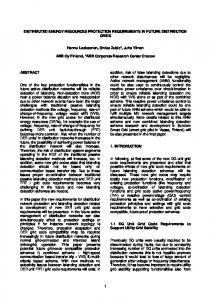
Comparing the timing of events in a system is impossible unless those events occur on a common timeline, meaning that the system has a common clock. To guarantee that timing constraints on events in a system are met, they must by scheduled against this shared clock (timeline). The trouble is that implementing shared clocks becomes nontrivial as physical system sizes and clock frequencies increase. Synchronous integrated circuits contain such shared clocks, implemented by carefully distributing a timing signal. In these systems, computation is broken down into blocks of logic, composed with intermediate latches to transmit data. Communication of data by latch from one logic block to another is triggered by transitions in the timing signal, and hence all communication and concurrent computations are aligned. A simple synchronous integrated circuit illustration is provided by Figure 1.1. This uniform scheduling of all computation and communication that is exhibited by synchronous integrated circuits is henceforth referred to as uniform time divisioning. In a synchronous circuit, as long as computations always complete between signal transitions, and as long as the clock signal is received synchronously by all latches, then all events can be precisely mapped onto a single logical sequence of discrete instants. Unfortunately, a distributed clock signal can never be received in perfect synchrony. No physical wires that transmit timing signals in a circuit can have exactly the same transmission delay, because there exist no manufacturing processes with perfect tolerances. This means that

2

CHAPTER 1. INTRODUCTION

data R

Logic A

data R

Logic B data

clock Figure 1.1: Simple illustration of a synchronous circuit, where communication between blocks of logic A and B is governed by a single uniformly distributed clock that triggers latches R.

mapping events into discrete time is always merely an illusion. Similar examples include the process of imposing binary values upon data — physical storage is inherently analog, but is logically carved into bits. Uniform time divisioning is thus the name for the illusion that time across a system is a sequence of discrete uniform instants. For systems with correctness specifications that explicitly bound reaction time, correctness validation requires uniform time divisioning. Formal verification is a validation process where correctness criteria are defined using formal logic, and system implementations are proven to meet these criteria. System validation can also include other approaches such as on-line testing and simulation, but formal verification provides the most conclusive indication of correctness and is therefore very desirable [36, 51]. Formal verification of temporal correctness for a system, proving that timing constraints will hold in the absence of physical system failure, is significantly more difficult when systems are not uniformly time divisioned [37, 8]. Unfortunately, implementing uniform time division by synchronously distributing a timing signal to many computing components across large distances is impractical, especially if the signal frequency is high. This has even become a problem for recent integrated circuits. Clock frequencies and chip sizes have grown to the point where the cost of clock distribution is becoming prohibitive. The overhead actually paid in commercially successful systems provides a good indication that hardware designers find uniform time division very valuable. In the DEC Alpha 21064 processor, 40% of the power is dissipated by the clock distribution network alone [41]. Once clock distribution becomes too expensive, multiple clocks can be employed, creating what is called a globally-asynchronous locally-synchronous (GALS) system [85]. Each clock then generates the timing signal for only a part of the system, called a synchronous timing domain, or simply a domain. Each domain may be independent, and may even have different frequencies. For example, in a network of general-purpose processors, each processor is likely equipped with its own clock. Because of physical factors, perfectly stable oscillator devices, meaning those where the average frequency is always equal to the actual frequency, do not exist [104, 70, 103]. This means that no two clocks are ever perfect synchronous, even if they have nominally equivalent frequencies. Hence, systems that span multiple domains and that require the assumption of system-wide discrete time must employ additional measures to reconcile fluctuations in

1.2. DISTRIBUTED REACTIVE SYSTEMS

3

their clock frequencies and thereby regain uniform time divisioning and the associated benefits like formal correctness verification. Large uniformly time divisioned systems are uncommon. Among those which exist, a prominent example is the SONET/SDH network, which forms the core of the global communications infrastructure [105]. Another example is the Time-Triggered Architecture for embedded hard-real-time systems [59]. Both of these examples achieve determinism using specialized techniques that to not readily transfer to other applications. The examples and their techniques are discussed with greater detail by Chapter 2. Consider that the market for distributed computing systems with deterministic timing is potentially vast. Many applications that use the Internet for communication today would prefer a more deterministic platform, provided it can be had cheaply enough [25, 26, 83]. Prominent examples include massive multi-player online games (MMOGs), where commercial success depends upon the real-time qualities of the user experience [20].

1.2

Distributed Reactive Systems

Pnueli defined reactive systems as those where the input and output timing of computations is determined by predictable external environment events to which the computations must react [78]. The implementation of computations is not important. The distinguishing property of reactive systems is the fixed timing of computations. Distributed reactive systems are defined as reactive systems that span multiple domains and where computations in one domain must interact with those in other domains to meet timing constraints [92]. In other words, timing constraints bind not only computations but also the communication between them. More formally, let a computation be self-contained if all inputs are available at the start of execution, meaning that execution can proceed without interruption until results are produced. Let a computation be reactive if it is self-contained and always terminates, and hence has known bounds on its resource needs. For brevity, let reactive computations also be called reactions. Let the definition of reactive system be restated more carefully as an iterating reaction over a sequence of input events, paired with sufficient resources to ensure that results are available within a known delay for each input event. In other words, a reactive system is one which “reacts” to its environment at the speed of the latter. These deterministic properties guarantee that the consumers of computational results can operate on a fixed schedule, never waiting. Contrast reactive systems with “interactive” ones, where consumers must tolerate unknown or unpredictable timing. Interactive systems operate at their own speed and not that of the environment. Neither reactive nor interactive systems are assumed to terminate, but they contain iterated computations which are individually assumed to. Obviously, only reactive systems are amenable to formal verification that they satisfy environmental timing constraints. This is because formal verification is a definite process, and nothing definite can be concluded about interactive systems; they have indefinite properties.

4


Reactive systems are convenient abstractions because they highlight determinism while hiding the details of what hardware and software mix is used in their implementation. Provided that a reaction has the proper timing, it may be implemented purely as hardware, as a program in a general-purpose instruction set, or as a shorter program in a domain-specific instruction set. The simplest reactions are blocks of boolean logic composed to create a larger circuit, an adder for example. The following sections discuss in detail what is required from implementations to qualify as reactive systems.

1.2.1

Software Determinism

To guarantee reactive properties for computations in software systems requires that sufficient resources are allocated to always ensure termination within associated time constraints and with correct results. A system can support a mixed workload of reactive and non-reactive computations as long as the non-reactive computations cannot interfere with those resources allocated to the reactions. Unfortunately, establishing the properties of software computations prior to their execution is often non-trivial. Consider a simple software computation that transforms a single body of input data into a single body of output data of equal size, and that is known to terminate. This transformational model of execution can be formally described using the following notation: fρ : x →τ x0

(1.1)

Read this to mean that a computation f transforms input data x into output data x0 over at most some discrete number of cycles τ , relative to a processor implementation ρ. Assume that a single memory region contains the input x prior to computation execution, and the output x0 afterwards. Also assume that this memory region initially contains (and hence that x contains) all necessary executable code for f . Treating code as a component of input data allows a single number to capture the entire memory resource needs of the computation. Thus, let the memory region which contains first x and later x0 be γ bits in size, such that it precisely matches the data size γ = |x| = |x0 |. Given these assumptions, define the profile for a computation as the resource quantities necessary to ensure execution until termination. A profile, a pairing of cycle count and memory amount for a given processor implementation, is well specified by the following simple tuple: (τ, γ)ρ

(1.2)

To illustrate reactions and their profiles, consider the following example, specified using the MIPS instruction set. lw $1, 16($zero) lw $2, 20($zero) add $3, $1, $2 sw $3, 24($zero) [lhs input word]


5

[rhs input word] [output word]

This program loads two words of input, adds them together, and stores the result. Data and code occupy a contiguous region of memory, based at memory address zero, where the input words are initialized with the input values for the program. Given the somewhat unrealistic assumption of single-cycle execution for all instructions, the profile is 4 processor cycles and 7 memory words. Just as profile notation can be used to fully specify the resource needs of transformational computations, it can also be used to specify the availability of resources themselves. Assume that resources in a software system have been uniformly time divisioned, meaning that a discrete timeline has been imposed upon all processors. During each unit of the timeline, the quantity of available resources at each processor is called a provision and is specified by a profile. One provision exists at each processor during each unit of time, and hence the frequency of provisions matches the time divisioning frequency. This notation for provisions and profiles allows a concise redefinition of reactive systems as those where all computations are allocated provisions with matching profiles, and where the provision frequency matches the maximum frequency of external events. Software reactions are thus transformational computations that have been allocated sufficient provisions. Because uniform time divisioning creates provisions at each processor with the same frequency, assume that reactions which have slower event frequencies can be allocated multiple sequential provisions and thus their execution frequencies matched to their events. Quantifying execution time using profiles assumes that processors have deterministic timing for all operations. Specifically, it assumes that each processor measures time in discrete units called cycles, and that the cycle duration for each processor operation is known. Unfortunately, this need for certainty in durations is at odds with modern processor architecture. Complex memory hierarchies and deep superscalar instruction pipelines can exhibit very unpredictable timing [71, 77]. Establishing timing bounds for some architectures may thus require conservative assumptions and result in poor efficiency. However, the picture need not always be so bleak. Examples exist where careful management of dataflow within a complex memory hierarchy has resulted in both predictability and improved performance [87]. Even when the durations of processor operations are assumed to be deterministic, establishing the profile for arbitrary software computations can be difficult or sometimes impossible. For example, the use of Turing-complete programming languages can greatly complicate the evaluation of computation profiles, as termination for these languages is undecidable. Notice that any computation can be forcibly made transformational by simply interrupting it at the time that results are needed, then taking as results whatever data it has managed to produce. Value correctness for these results is obviously not guaranteed by this method. Verification that computations are reactive requires guaranteeing proper termination within the profile specified resource budget. This issue has received a vast amount of research effort, and is generally referred to as worst case execution time (WCET) analysis [49, 77, 16, 76, 43, 71, 91, 74].

6


An alternative approach is to restrict the software programming model to ensure that computations are always deterministic. For example, boolean circuits of finite size form a model of computation that captures all decidable languages [102]. The intuition here is that any terminating computation on inputs of bounded size (i.e. the simulation of a Turing machine decider) can be implemented as a finite boolean circuit. Specialized languages have been developed with such restrictions for the purpose of designing reactive computations [37, 102, 2, 50]. Specifically, Esterel [17, 18], Lustre [45], and Signal [44] form a family of “synchronous languages”, which reflect what is called the “synchronous/reactive” model of computation [46]. These languages have had commercial success with safety-critical systems such as avionics, automotive control, and nuclear power plants [15]. Indicative of the nebulous boundary between reactive hardware (boolean circuits) and software, systems specified in these languages can be compiled into either form. The primary focus of the synchronous languages is centralized systems where communication between concurrent computations is instantaneous [14]. Extension to distributed architectures is straightforward, provided that communication is synchronous [22]. In short, communication channels with non-zero latency can be represented as multiple stages of computation, each of which simply implements the identity function. An alternate but equivalent abstraction is fixed-length first-in-first-out queues for each communication channel. Popular alternatives to the synchronous languages include StateCharts and its derivatives, which provide a graphically oriented framework for specifying reactive systems [48, 6]. Also available is Charon, a newer language designed around the reactive formalisms of Alur et al. [1, 4, 3]. Other options for creating reactive components include hardware/software co-synthesis systems, such as Chinook [24].

1.2.2

Communication Determinism

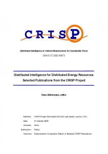
For a uniformly time divisioned reactive system, communication can be abstracted as a sequence of reactions that apply the identity function to their data. The length of this sequence is fixed over time and is determined by the latency of the communication channel in units of shared discrete time. An alternative but equivalent abstraction for communication channel is FIFO queues of static length and width, matching the latency of the channel and the quantity of data to be exchanged, respectively. These abstractions apply equally to communication between reactions themselves as to communication between reactions and devices that interface with the external environment. The abstractions are also indifferent to the mixture of hardware and software used in the implementation of a system. This should seem natural, since software reactions (provisioned transformational computations) in a uniformly time divisioned system are the software analog to computational logic blocks in synchronous circuits, and are computationally equivalent. An simple such system is illustrated by Figure 1.2. This dissertation assumes that sensor and actuator devices are logically equivalent to one-ended or one-sided hardware reactions, meaning ones that behave like reactions

7


data

A

B

clock

Figure 1.2: Illustration of two processors in different independent timing domains, but which operate synchronously like blocks of synchronous logic (see Figure 1.1) while communicating over potentially large distances. Each dark square indicates a data result. Using the techniques proposed in this dissertation, the shared clock signal is not actually distributed, but instead independently calculated by each processor.

where either the input data or the output data lies outside the system. These device reactions must share the same uniform discrete timing as all other system reactions. Device reactions are assumed to support arbitrary device functionality, provided that the rate of input or output (as appropriate) and the data quantities are deterministic. Most common devices can be categorized as converters between continuous and discrete data streams (analog and digital). Such processes are naturally deterministic, involving fixed sample frequencies and fixed sample sizes. For pure hardware systems, meaning those that have only static computations implemented directly in logic and no programmable processors, implementation of these communication abstractions is straightforward. At the granularity of individual domains, integrated circuit components are readily available that correspond precisely with the abstraction semantics, such as latches and FIFOs. At larger granularities, there are no commonly available “off-the-shelf” solutions. There exist several time divisioned communication protocols, but their timing is either not uniform or it is not trivially conscripted into the role of also time divisioning computations. Addressing this shortcoming is a primary goal of this dissertation, and is addressed in detail by Chapter 3. The drawbacks of existing approaches is discussed by the next Section and by Chapter 2. For software systems, meaning those with programmable processors, the transformational execution model already includes communication resources in profile specifications implicitly. Because transformational computations neither consume nor produce intermediate data, everything is captured by the profiled memory resources and need not be otherwise distinguished. The actual communication or exchange of data occurs between instants on the shared timeline. The input data for each reaction is really just a union of received communication data and the program code for the reaction, as specified by the preceding section. The “persistent state” for a reaction, meaning the data that a given reaction needs during each iteration of its execution, is best thought of as communication data between earlier and later instances of that reaction. Results of reactions must similarly include all data that is to be exchanged with other reactions or with devices. In this manner, communication is logically instantaneous from the perspective of reactions.

8

1.3


Clock Synchronization

Faced with the problem that a distributed system spans multiple timing domains, one approach to establishing a shared definition of time is to align each domain with an reference clock that lies external to the system. By definition perfect synchronization is impossible, as explained by Section 1.1. The remaining result is approximate synchronization. Synchronizing multiple clocks to a single absolute (Newtonian) time reference is called clock synchronization or network synchronization. This process continuously corrects the drift between the local clocks in each domain and a centralized reference (such as UTC via GPS) with bounded accuracy. Clock synchronization has been exhaustively researched and is well understood [5, 72, 34, 33, 65, 88, 94, 99, 97]. Implementations such as NTP are widely deployed [81, 82]. Clock synchronization is an example of a distributed algorithm to establish global shared state in a distributed system. The term distributed consensus is commonly used to categorize the goals and properties of this and similar algorithms. Important limitations of distributed consensus have been discovered. Most relevant to this discussion is that distributed consensus becomes both highly complex and expensive if the system must tolerate the failure of physical components or of computations. The important “FLP result” showed that even a single failure is sufficient to always prevent consensus in an asynchronous system [40, 32]. Fortunately, this great weakness can be overcome in practice, because manufacturing tolerances bound the maximum frequency difference between nominally equivalent oscillators that are functioning properly. Expressed more formally, domains with nominally equivalent oscillators are merely plesiochronous, only appearing asynchronous when they have physically failed. However, if components can fail in a methodically destructive or malicious manner, much additional complexity is introduced. Such extraordinary faults are referred to as Byzantine, after Lamport’s famous Byzantine generals analogy [66]. Note that Byzantine failures need not always imply attack by an adversary — they are known to result from simple programming errors. Clock synchronization is a continuous process. Distributed consensus must be repeated at regular intervals to compensate for changing oscillator frequencies. Those synchronization implementations that are robust to Byzantine failure are often also burdened by the strong assumption that all clocks in a system are initially synchronous. Obviously such an assumption is impractical, especially at large scales. A recent approach by Daliot et al. addresses this by abandoning the use of an external reference [27, 28]. Instead, consensus is achieved for a value derived from the clocks inside the system. This relaxation allows for significant performance improvements. However, it does not address the cost of consensus itself. An alternative approach is to eschew absolute time and focus on aligning the rate at which time appears to pass within each domain, and thereby ensuring that all domains experience a common timing signal. From this perspective, the frequency fluctuations caused by the environment can be treated as noise that obscures this shared timing signal, not unlike noise on communication channels. Just as communication signals can be recovered despite noise by leveraging redundancy in data encodings [100], a shared timing signal can be recovered by leveraging oscillator redundancy. In a system with multiple

1.4. CONTRIBUTION

9

oscillators that all provide approximate measure of the same value (physical time), and where differences between their approximations are independent, combining their measurements can lead to a better approximation. This dissertation proposes techniques that leverage these intuitions.

1.4

Contribution

This dissertation makes a contribution in two parts. It proposes metasynchronization, a technique to uniformly time division all resources in distributed systems that span multiple timing domains. It also proposes hierarchical provisioning, an execution model that leverages uniform time divisioning to improve the functionality of and simplify the infrastructure for general-purpose distributed computing. By focusing exclusively on uniform time divisioning without regard for clock synchronization, metasynchronization can be significantly more efficient and robust than systems which require the latter (possibly to implement the former). Unlike clock synchronization, uniform time divisioning is not inherently centralized and can be guaranteed without agreement on absolute time. THESIS (part 1 of 2): Distributed computing and communication resources with independent local timing can be uniformly time divisioned in a completely decentralized manner. Metasynchronization partitions time into a uniform sequence of metacycles, with durations larger than the cycles of any local oscillator. Metacycles cannot map one-for-one with individual oscillator cycles, as this would preclude tolerating any natural frequency fluctuations. Instead, metacycle synchronization is achieved at a coarser granularity. The envelope within which oscillator frequencies vary is usually specified by the oscillator manufacturer. Improving production techniques are constantly reducing the cost of greater oscillator precision. For example, a common quartz oscillator may experience frequency variations of up to 10 parts per million (ppm), meaning that it stays within 0.001% of its nominal frequency under regular operating conditions [104]. To illustrate this further, consider an oscillator with frequency specification of 100 MHz ± 1000 Hz. When functioning properly, this oscillator may produce signals between 999, 999, 000 Hz and 100, 001, 000 Hz during any given second. The exact frequency function is assumed to be unpredictable. For each oscillator, define its nominal duration as the number of local cycles (and fractional cycles) that would occur during every metacycle if the oscillator were operating at precisely its nominal frequency. Define the logical duration for each oscillator as the minimum number of local cycles that are guaranteed to occur during a metacycle. In other words, the logical duration is the nominal number of cycles which occur during a metacycle, minus the maximum variation in cycles over that period. Finally, define the the physical duration for each oscillator to be the actual number of local cycles which actually do occur during a specific metacycle. This value changes over time but is always greater than the logical duration.

10


Metasynchronization is achieved independently for each oscillator by depriving computations of all extra cycles beyond the logical duration. Hiding extra cycles from computations in this manner makes oscillators appear to always operate at precisely their logical frequency. Although discarding extra cycles may initially seem inefficient, the tiny range of frequency error for actual oscillators means that cost in practice is usually negligible. The exact number of extra cycles depends upon the physical duration and hence varies with time. Accordingly, the duration of metacycles is calculated independently for each domain and reconciled over time with the changing number of extra cycles. To calculate this number, each domain in the system passively observes its neighbors to discover changes in the relative timing between them and thereby to estimate local fluctuations and to correct for them. When the extra cycle estimation is successful in all domains, the metacycle frequency at each oscillator will match that of its neighbors in the network, and the system as a whole is said to be metasynchronous. Because extra cycles cannot be directly measured and instead are only estimated, local fluctuations cannot always be accurately corrected. However, the average neighbor algorithm presented in Chapter 3 can guarantee that local fluctuations are temporary and can be hidden from higher levels. Such completely decentralized control processes are commonly referred to as self-stabilization [31, 61, 42]. In this manner, metasynchronization reliably provides the illusion of synchronous discrete time for the entire system. For further illustration, consider the following simple example. Suppose that two oscillators are able to observe one another and to calculate differences in their frequencies over time. Let both oscillators have equal frequency specifications of 100 MHz ± 1000 Hz. Let the metacycle frequency be 1 KHz, such that both logical durations are 999, 999 cycles. During each metacycle there can occur between 0 and 2 extra cycles at each oscillator, depending on the changing physical durations. The goal of metasynchronization is that, from the perspective of each domain, frequency equality can be guaranteed such that 999, 999 local cycles occur for each 999, 999 cycles at the other oscillator. This equality for granularities larger than single cycles is the guiding concept behind metasynchronization. The granularity must be larger than one to allow for fluctuations. In fact, the degree to which the granularity must be larger is a direct function of the maximum fluctuation amount. By using a self-stabilizing process, metasynchronization completely avoids the dilemma of distributed consensus and can be implemented both more efficiently and more robustly than clock synchronization. Each timing domain can tolerate the simultaneous malicious (Byzantine) failure of multiple neighboring domains without risk of disrupting its own synchronization to the metaclock. The only resources sacrificed as overhead to the metasynchronization process are small receive buffers for each link. More detailed performance and robustness evaluation is found in Sections 3.4 and 3.5. As discussed by Section 1.2, practical techniques to impose uniform time divisioning allow straightforward implementation of large distributed reactive systems. However, uniform time divisioning can also be useful for general-purpose distributed computing, where resources are shared by arbitrary untrusted computations. To support reliable execution under such circumstances, systems must isolate computations from one another.

1.5. DISSERTATION PLAN

11

Virtualization is a popular and conceptually simple isolation technique, where a single real execution environment emulates multiple copies of itself. Computations in different execution environments are limited in their ability to interfere with one another because the actual sharing of resources is hidden from them. On personal computers, for example, hypervisor virtualization allows multiple unmodified operating systems to transparently share a single physical machine [12, 30]. Virtualization can be implemented with varying degrees of fidelity, and is perfect only when computations are unable to detect any differences between emulated and actual execution environments. A perfectly virtualized processor must have performance properties indistinguishable from a physical one, for example. THESIS (part 2 of 2): Uniformly time divisioned software systems can support perfect virtualization, and thereby allow resource sharing by arbitrary computations with deterministic performance. The hierarchical provisioning execution model is introduced by Chapter 4 to prove this claim, and is based on the simple provision resource model defined by Section 1.2.1. The intuition behind the model is that a single provision can serve as a host for nested provisions, each of which spans only a subset of the host resources, including processor cycles. In turn, this allows an arbitrary collection of computations to be encapsulated within a single root provision, which conveniently corresponds to the resource semantics imposed by uniform time divisioning. Because it provides perfect virtualization, the model preserves execution determinism for all provisions in the hierarchy, meaning that the timing for all execution preemption is known in advance. This enables all computations to implement any scheduling policy they wish by creating nested provisions for their subcomputations. The root provision is guaranteed by the model to be executed with equal resources during each system time step. The iterated execution timing of nested provisions depends upon the scheduling policies imposed by their host computations. In other words, the model only guarantees deterministic timing for the root — to support deterministic time for guest computations, reactions for example, requires that all computations in the hierarchy on the path to the root schedule them deterministically (statically). Contrast this scheduling flexibility with the centralized policy arbitration that is necessary in systems with traditional operating system kernels and privileged processor modes. Implementing the execution model and thereby enabling perfect virtualization requires isolation mechanisms that enforce provisions. Chapter 4 makes the case that such mechanisms can be efficiently implemented in hardware, which implies that hierarchically provisioned systems have no need for privileged software of any kind.

1.5

Dissertation Plan

The rest of this dissertation is organized as follows. Chapter 2 reviews related work, providing helpful context for the technical material of later chapters.

12


Chapter 3 introduces the metasynchronization technique, and evaluates its feasibility. The technique itself is based on three simple rules that govern the computation and communication of each processor in the system. However, to obey the rules requires self-stabilization of oscillator frequencies that naturally vary over time. One specific such algorithm, called the average neighbor algorithm, is presented in detail. Metasynchronization imposes negligible communication overhead by design, and the average neighbor algorithm has a fixed small computational footprint. Memory for communication buffers is the most significant overhead expense imposed by the system, and also the most complex to predict. Simulation results are provided to show that the expected memory footprint is also minimal under practical conditions. Chapter 4 introduces the hierarchical provisioning execution model, which allows deterministic sharing of resources by arbitrary untrusted distributed software applications. This model is first formally specified, and then contrasted with models used by conventional systems. Examples are provided to illustrate the practicality of the model for common tasks, and implementation strategies are discussion. Chapter 5 summarizes the contributions and concludes with speculation about promising directions for future work.

13

Chapter 2

Related Work There have been many efforts to impose and leverage synchrony for systems larger than integrated circuits. A discussion of those efforts most relevant to this dissertation follows.

2.1

Logical Event Clocks

Some applications are indifferent to physical time, but still depend on a time reference to manage relationships between their components. Instead of dealing with the complexity of clock synchronization, these applications can define time in a purely logical manner, independent of physical time, by focusing only on the ordering of application events. Lamport [62] introduced event-based time to distributed systems and defined the happened before event relation to partially order events. Given any discrete measurement of time, it is not generally possible to impose a total ordering on all system events. Processes in a distributed system operate concurrently, meaning that events may occur simultaneously within multiple processes. Thus, the happened before relation can impose only a partial order. Lamport also defines logical clocks as those relations between simultaneous events which extend happened before to totally order events, possibly arbitrarily. There can be multiple logical clocks for a system, as only the partial ordering is uniquely determined by system events. Metasynchronization can be thought of as establishing logical time, in that it does not rely on any external time reference and hence is in principle independent of real-time. Any uniform time divisioning process naturally must impose a partial event ordering upon the concurrent events in a system. However, unlike creation of a purely logical clock, metasynchronization does approximate real time. The accuracy of this approximation is a function of the stability of the oscillators in the system. Further, metasynchronization spans all components, including the sensor and actuator devices that interface with the real world, allowing physical time constraints to be met. Isotach networks are a particularly interesting approach to providing logical clocks, specialized for tightly coupled parallel computers [89]. A key feature of isotach networks is that the logical timing of communication can be precisely controlled. The sender of a message can control the logical time at which the message is received. Isotach logical time is defined as a tuple of integers. One of these integers reflects a “pulse” count, which is globally shared, and is quite similar to the metacycles imposed by Metasynchro-

14

CHAPTER 2. RELATED WORK

nization. However, isotach pulses are technically independent of physical time; they are established with explicit communication. Furthermore, the current definition of isotach networks is intolerant of any component failures.

2.2

SONET and SDH

The Synchronous Optical Network (SONET) protocol [105], and the closely related Synchronous Digital Hierarchy (SDH) used outside the US, form the foundation protocols for most of the global telecommunications infrastructure. As alluded to in Chapter 1, these protocols impose uniform time divisioning upon a communication network. Specifically, SONET is designed around a process called synchronous multiplexing, which depends on the synchronous time divisioning of communication to coordinate the intersection of multiple communication links at each node in its network. In brief, data is encoded on each network link in such a way that “frames” of data can be switched between the links intersecting at a node based solely on time, not based on any in-band signals. Switching SONET frames occurs at 8KHz on all nodes, meaning that frames are read from all network links during each interval of 125us. The data within these frames is then demultiplexed, possibly reordered across multiple frames, and finally multiplexed and transmitted again. This process only works if exactly the right amount of data to form a frame is available at each node during each interval. If an upstream node were to transmit slowly and send less than the expected amount of data during an interval, the time-based demultiplexing will fail and result in communication failure. To synchronize communication, SONET depends on both the distribution of a single “master” clock signal and on synchronization of local clocks at each node. This process is similar to making a single clock available across a digital circuit, but is adapted for the physical scales of a global system. Each network has a clock that is transmitted across the system together with data. This clock governs the time divisioning of resources. Interestingly, the synchronization is imposed only on the communication between SONET components; it is invisible to the end-users of the system. In fact, the protocol includes facilities to track the timing of user communication channels, called “tributaries”, allowing them to have timing independent of the SONET system. Timing in SONET is highly complicated and therefore some of the details must be omitted here. The primary goal is to achieve the level of reliability required of public telecommunications infrastructure, generally referred to as “five nines” of reliability, meaning that the system should be usable 99.999% of the time. Local clocks help this by providing timing redundancy. Each node has a highly accurate and reliable local clock, combined with dedicated communication bandwidth on each link for a clock synchronization protocol. To mitigate the cost of expensive accurate clocks, there are multiple tiers of clock quality. The goal of clock synchronization is to allowing for reliable operation during periods where communication fails or reference clocks become unavailable. SONET experiences a significant drawback by synchronizing to a single timing reference, which is called the “mid-span meet” problem. The issue is that each commercial

2.3. SYNCHRONOUS OVERLAYS

15

telecommunications provider is inclined to use a different timing source for its own network. This greatly complicates the seamless exchange of data between independently operated networks, and a surprising amount of the protocol standard is dedicated to its resolution. The metasynchronization techniques proposed in this dissertation avoid this problem entirely by being fully decentralized. Although SONET is a highly successful architecture, being used nearly universally in global telecommunications, it is too “brute-force” to transfer well to other application domains and different time scales. SONET synchronization is expensive, especially when redundant high quality clocks are needed for robustness. Metasynchronization provides an alternative algorithmic approach, which is highly robust while tolerating inferior clocks. Thus, it can be deployed on a larger set of implementation platforms. It can also be tuned to different synchronization granularities, which can allow application at both small and large scales.

2.3

Synchronous Overlays

A synchronous overlay tries to provide higher level applications with the illusion of logical synchrony, while being implemented using asynchronous packet forwarding. The goal is not meeting physical time constraints, rather taking advantage of the reduced concurrency management complexity that is enabled by synchrony. This is only a weak form of synchrony as it can be used to organize applications, but not meet real-time constraints or optimize resources (e.g. synchronous circuits need no communication buffers). In fact, this weak synchrony is in principle equivalently powerful to asynchrony [23]. A number of research efforts have addressed this issue from various angles [10, 90, 98, 53, 19]. However, all of these approaches have significant drawbacks. The greatest of these is poor fault tolerance, specifically intolerance of Byzantine failures. The only exception is a class of “pulse-based” synchronization techniques, where a self-stabilizing approach is used to combat Byzantine behavior [11, 35, 28]. However, even these system suffer from significant communication overhead. All of the frameworks rely on some form of “control” or signaling messages between components for synchronization, and hence face the risk that this signaling is performed incorrectly by a component as the result of programming error, failure, or malicious intent. Dealing with such Byzantine behavior is proven to be very complex and expensive, which likely explains why none of the cited systems do so. Even if faults can be tolerated, scalability is troublesome. Broadcast causes control message volume to grow non-linearly with system size. Metasynchronization can address both the possibility of traitorous behavior and communication overhead scaling by entirely avoiding the use of control messages. Instead, the implementation requires that nodes in a network can directly witness the timing behavior of their neighbors — which rules out layering as an overlay above networks such as the Internet. Avoiding explicit messages is critical, as Awerbuch [10] has formally established a significant minimum communication overhead for addressing this problem at

16

CHAPTER 2. RELATED WORK

the overlay level. The immunity of metasynchronization to Byzantine faults is described more precisely in Section 3.4.1.

2.4

Real-Time Scheduling

Systems are commonly called real-time if their correctness depends both on computations producing expected results and on these results being available at expected times. Such timing constraints, or deadlines, are said to be hard if failure of the system can cause negative consequences in the physical world. The field of real-time research obviously shares many of the stated goals of this dissertation. To evaluate the details of the relationship, consider that real-time systems can be divided into two classes based on their approach to scheduling. When applications that share a system compete for resources, depending on the scheduler, this may result in conflicts or contention. Conflicts can then either be prevented from occurring, or they can be resolved dynamically once they occur, hence two categories [21]. A great deal of research has focused on “real-time scheduling”, which generally refers to the dynamic resolution of conflicting demands for resources [75, 9, 54, 101, 106]. This approach is applied primarily to centralized or non-distributed systems because coordinating a dynamic scheduler across long-latency communication links is impractical. Once system state information arrives at a scheduler from far away, it is likely already out-of-date. However, dynamic approaches cannot be avoided entirely in a general purpose system, since they are necessary for efficiently dealing with those applications that have unpredictable resource needs. Instead of dynamically resolving conflicts, an alternative approach is to statically allocate resources and to restrict the set of applications accordingly with some admission control policy [55]. This approach corresponds most obviously with uniform time divisioning, where resources are naturally partitioned into units that can be easily preallocated.

2.5

The Time Triggered Architecture

An existing system that illustrates the static approach to the construction of real-time systems is the Time Triggered Architecture (TTA) [59, 57]. The TTA is intended for highdependability environments, also known as hard-real-time or safety-critical. It provides a set of techniques for building distributed systems in a highly static manner to allow for strong confidence that all deadlines will be met. The hardware is assumed to be customized for and dedicated to an application. A combination of clock synchronization and dynamic adjustment of clock rates is used to create a global time reference. The TTA approach has many similarities with the metasynchronization approach, in that it also seeks to identify and isolate oscillator variations [58]. However, the TTA approach is less concerned with scalability and hence adopts a centralized approach to identifying frequency variation. The TTA is synchronous

2.6. TEMPORAL LOGIC

17

at the granularity of “macroticks”, which correspond to metacycles in this dissertation. A subset of the nodes in the system are categorized as “rate masters” with high-stability oscillators, which together participate in traditional clock synchronization. Other nodes are divided into “clusters”, such that each cluster contains a master. Non-master nodes then derive their own rate changes by adapting to the rate of the master, which they can measure directly through communication. This is basically the same method used by metasynchronization on all communication links. Metasynchronization has the advantage over this system of being completely decentralized and self-stabilizing, which allows it to avoid the need for high-stability oscillators, to tolerate simultaneous node failures, and to avoid the need for any traditional clock synchronization.

2.6

Temporal Logic

Temporal logic is a form of modal logic which has been specialized for reasoning about relationships in concurrent systems, specifically the change in truth of assertions over time [37, 64]. Temporal logic operators include sometimes and always, in addition to those of traditional boolean logic. These operators inherently assume that systems are synchronous, that a single measurement of time applies everywhere in a system. Temporal logic is widely used in specifying and verifying the correctness of applications for synchronous systems. By making synchrony more practical for a wider range of applications, metasynchronization helps to enable wider use of temporal logic, hopefully leading systems to become more correct and reliable.

18

Chapter 3

Metasynchronization “... if a distributed system is really a single system, then the processes must be synchronized in some way.” — Leslie Lamport [63] The aim of metasynchronization is to temporally partition both the computations and the communication of an arbitrarily large distributed system at a fixed metaclock frequency. This process is complicated because no two independent sources of time ever agree perfectly, and because uniformly distributing the signal from a single timing source is neither robust nor scalable. This chapter introduces a set of techniques to enable synchronization analogous to that of synchronous integrated circuits, using only independent imperfect timing sources, and at arbitrary scale. Metasynchronization works by having each independently timed domain in the system locally identify and correct timing irregularities by watching incoming communication from neighboring timing domains. For simplicity, timing domains are referred to as processors below, although there is no formal requirement preventing several processors from sharing a time source, nor a requirement that these processors be software programmable. Although processors have direct access only to their own oscillators, they also have indirect access to those of neighboring processors, via data signal timing across shared communication links. Given properly structured communication, processors can compare their own frequency with that of their neighbors to measure differences between them. Unfortunately, even once a processor has established that a difference in timing exists between itself and a neighbor, it cannot know if its own timing or that of the neighbor has changed, or both. Similarly, if a processor has multiple neighbors, the timing difference may vary for each one. It turns out that a simple self-stabilizing solution, referred to here as the average neighbor algorithm, allows each processor to adjust its frequency over time to match that of its neighbors, with the result that global synchrony emerges. As the name suggests, the algorithm involves each processor adapting to a single hypothetical average neighbor, which is the aggregation of its actual neighbors. Section 3.3 shows that this simple decentralized technique causes rapid frequency convergence regardless of network topology. The overhead costs of metasynchronization depend on how rapidly synchronization is achieved. Only negligible bandwidth is sacrificed, but each communication link requires dedicated buffering at the receiver, which imposes both memory and latency costs.

19

3.1. THE THREE RULES

Because stabilization is normally very rapid, this overhead can be kept to a minimum in practice. The algorithm is implemented independently at each processor using only local information, calculating frequency adjustments at regular steps on the timeline of metacycles. This discrete behavior allows the frequency state of each processor at a given time to be represented as a simple linear equation over its previous state, and hence the entire network as a system of such equations. This facilitates mathematical reasoning about the system and formal verification of the algorithm properties, such as resistance to failure and frequency stabilization time.

3.1

The Three Rules

For the sake of precision, formally define the desired effect of metasynchronization as follows. Let a network be a distributed system of processors, which are connected using bidirectional point-to-point links. Let neighbors be those processors which share links. Processors communicate by sending message frames to their neighbors, the size of which is determined by the corresponding link bandwidth. Formalize this definition of processors P and their neighbor sets ηi as follows: P = {pi | processor(i)} ηi = {pj | link(pi , pj )}

(3.1) (3.2)

Let a network be metasynchronous when communication between any pair of processors coincides with the communication between all others. This divides communication into metacycles which are perceived equally by all processors, and thereby establishes a shared metaclock — a global logical ordering of communication events. The following rules are obviously sufficient to impose this synchrony: RULE symmetry : Communication between any neighboring processors A and B must occur as a sequence of symmetrical message exchanges. At any time, the number of frames sent from A to B must (approximately) equal the number sent from B to A. The difference may temporarily vary by a single frame. RULE yoke : Frames must be sent in equal number by a processor to all of its neighbors. For a processor A with neighbors B and C, the number of frames sent to B must equal, again within single frame tolerance, the number of frames sent to C. RULE isochrony : Frames must be sent by each at a constant frequency (isochronously).

20

3.1.1

CHAPTER 3. METASYNCHRONIZATION

Logical and Physical Synchrony

Define a network to be logically synchronous if all processors observe an equivalent number of frame exchanges with their neighbors. The symmetry rule is sufficient to create logical synchrony for two processors. Applying only symmetry between all neighboring processors would establish independent shared orderings for each link. Processors would not be able to reason about timing relationships with non-adjacent processors, however. The yoke rule aligns orderings across the network, creating an eternal sequence of atomic steps, which are referred to here as metacycles, such that processors communicate with each of their neighbors during each metacycle. Logical synchrony is unfortunately not very useful in practice. Symmetry and yoke alone are intolerant of communication faults, meaning circumstances where a link or processor becomes unable to transmit frames, or where frames are lost. Without an isochrony constraint, communication faults result in starvation, where all processors may wait forever for frames and the system as a whole will cease to communicate. Specifically, the destination processors for any missing frames cannot known when to expect them, and thereby will interrupt the global frame exchange cycle. This need for physical synchrony to tolerate failure is well understood and holds for all concurrent systems: “In programming asynchronous multiprocess systems, the customary approach has been to make process synchronization independent of the execution rates of any components. This requires synchronization algorithms in which one process must wait for another to do something before it can proceed. In distributed systems, this means waiting for a frame from the other process. These time-independent algorithms cannot be fault-tolerant because a process could fail by doing nothing, and such a failure manifests itself only as a reduction of the process’s execution rate.” — Leslie Lamport [63]

3.1.2

Link Bandwidth and Latency

Metasynchronization only imposes rules on communication; it does not send any data itself. Frames are simply fixed-size fixed-rate containers for untyped higher level data. Metasynchronization requires that links be deterministic, with fixed latency and fixed bandwidth. This allows each link to transmit a fixed size frame during each metacycle. To maximize the bandwidth available for payload data, choose the frame size for each link to match the available raw bandwidth. Assume that either sufficient payload data is always available, or that shortfalls can be filled in with zeros (or random filler). Importantly, because frames are of fixed size, they need not contain any signaling overhead! Receiving processors need only count bits to know when a complete frame has arrived, and thereby also know when the next frame starts.

3.1.3

Link Initialization

Before the synchrony rules are applied, each processor must perform link initialization to fill the delay-bandwidth product of each link, that is, “priming” them with frames.

3.2. TIMING NOISE

21

This bootstrapping relaxation of the synchronization rules is necessary to fully utilize bandwidth. If the rules were applied immediately to empty links, each link would be limited to a single frame in each direction per round-trip time, a significant performance limitation. Because the rate of frame exchanges must be equivalent for all links (yoke rule), the throughput of all links would be further bounded by the maximal link delay — the link with the longest propagation delay must finish its frame exchange in lock-step with all other links. During the initialization phase, processors transmit frames but perform no receive processing. This process addresses the inequality between links with differing propagation delays, and allows longer links to have more frames “in flight” than shorter links. As explained in Section 3.2.2, received data on each link is held in buffer memory prior to consumption by the destination processor. These buffers are said to be balanced when precisely half filled with data. Processors should begin processing received frames for each link once balance is achieved. It is therefore unnecessary for processors to know link capacities (delay-bandwidth products) to perform initialization.

3.1.4

Conservation of Frames

Once links are full, the rules are imposed and the number of in-transit frames for each link remains constant, imposing a “law of conservation of frames”. When a frame is removed from a link in one direction, another must be added in the opposite direction. For readers familiar with the Internet protocols, this constraint is quite similar to the desired equilibrium behavior of TCP [93]. To ensure robust behavior during congestion, conservation of packets is referred to as self-timing by the packet networking community [52]. The goal is matching the generation rate for packets on a connection to the consumption rate.

3.2

Timing Noise

If processors were able to perfectly obey the isochrony rule, communication faults could be easily identified and tolerated. At the end of each metacycle, if a frame has not arrived on each link, processors expecting the missing data can assume a fault has occurred and simply abandon the link in question to maintain communication with their other neighbors. Unfortunately perfect isochrony is impractical and actual metasynchronization fault-tolerance is more complex. Assume that each processor has access to an independent local oscillator, from which both its communication and computation frequencies are derived. The word clock is henceforth intentionally avoided, to highlight that only frequencies and durations are needed for timing, not any specific counter values that refer to absolute time. Despite nominal isochrony, the waveform produced by any oscillator will vary naturally over time due to effects from its physical environment, such as temperature fluctuations. Manufacturers of oscillators generally publish these performance properties for their products [70]. Let the nominal frequency of the oscillator for each processor i be

22

Frequency


Nominal

Actual

Time

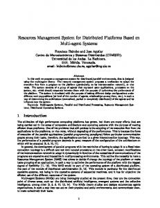
Figure 3.1: An example visualization of frequency variation over time. If frequency variation exceeds the light envelope and strays into either dark region (too fast or too slow), than the associated oscillator is defined to have failed. The size of the envelope is specified by the manufacturer.

defined as ωinom cycles per second. To account for frequency noise over time, allow the actual frequency for an oscillator to wander within a bounded envelope around its nominal frequency: ωiact (t) s.t.

(ωinom − εi ) ≤ ωiact (t) ≤ (ωinom + εi )

(3.3)

This says that the actual frequency ωiact (t) of the oscillator at processor i, in cycles per second (possibly fractional), is a function of time over the bounded range ωinom ± εi , where εi is the maximum instability (frequency error), as specified by the oscillator manufacturing specification. Outside this range, an oscillator and its associated processor are defined to have failed. Properly functioning processors in a system are expected to abandon communication with failed processors (and also abandon obedience to the associated synchronization rules) as soon as they can be identified as such. To illustrate this further, consider the simple example of two processors A and B with equal nominal frequencies of 100 MHz, and instability of 20 ppm. Assume that metacycles are locally defined to occur each 1 M cycles, meaning a nominal metacycle frequency of 100 Hz. Suppose that comparing the actual frequencies of A and B with a perfect reference frequency has A operating somewhat fast at 1 M + 7 cycles per “real” metacycle and B somewhat slow at 1 M − 3. This means metacycles at A occur slightly more frequently than metacycles at B, despite both internally counting metacycle duration with an equal number of (local) cycles. Such a difference becomes problematic if it persists for more than 1000 seconds, as A would advance an entire metacycle ahead of B with respect to real time.

3.2.1

Jitter and Drift

The following classification of timing noise is derived from Messerschmitt [79], which is recommended as a reference for the standard (but potentially confusing) terminology used to discuss synchronization. When comparing the frequencies of two oscillators, define them to be mesochronous if they share the same average frequency, but have individual cycles that are occasionally

23

3.2. TIMING NOISE

jitter isochrony Figure 3.2: Comparison between two data signals: an isochronous one where units are evenly spaced, and one with jitter.

out of phase (not be perfectly aligned, i.e. “jittering” back and forth). Accordingly, define jitter as the difference between two mesochronous frequencies. Define two frequencies to be plesiochronous if they are nominally equal, but do not actually share the same average, having diverged over time with no reasonable expectation of re-convergence. Define drift as the difference between plesiochronous signals. Notice that these definitions embrace all forms of difference between nominally equivalent frequencies, including traditionally distinct classifications such as skew. The point is to segregate noise based exclusively on the timescale over which it manifests, highlighting the need for entirely dissimilar correction techniques in the cases of temporary and of ongoing differences. The details of these techniques are presented in the following Sections. Given this perspective, jitter and drift are the same thing, the distinguishing factor being the duration over which frequency differences are considered. In colloquial terms, nominally synchronous frequencies progress from mesochronous to plesiochronous depending on how “out of whack” they actually are. To give an example, two signals generated by a single oscillator but traveling along separate paths of nominally equal delay will nevertheless experience some jitter due to physical differences in those paths, but will not experience drift since they share the same source. On the other hand, signals generated by independent but nominally equivalent oscillators can be assumed to be plesiochronous (to have drifted from the nominal frequency). There is also the further classification of heterochronous frequencies, meaning those with nominally different frequencies, where synchronization is obviously not possible.

3.2.2

Buffering Allows Two-Timing

Abstractly, all communication links are simple FIFO queues where enqueuing of frames by the sending processor can happen at an independent frequency from dequeuing by the receiver. This independence is necessary, since timing noise (jitter and drift) makes true synchrony for these frequencies improbable. The actual implementation of links is immaterial, so long as this abstraction can be met. For example, if both processors and the link are within a single integrated circuit, the standard logic for such FIFOs can be used directly. At larger granularities, such as for a long-distance link over optical fiber, extra receive memory is set aside at each end of the link and specialized hardware is dedicated to transferring the arriving data

24


from the fiber to the buffer. This hardware can then be timed by arriving data itself, for example by using a phase-locked loop (PLL). In all cases, some memory is needed to provide the necessary isolation between data production and consumption frequencies, and henceforth is referred to as buffer memory. Frame transmission frequency is derived from the local oscillator frequencies of the source processor. Assume that each processor can and does both produce and consume exactly one frame for each adjacent link during each metacycle. It does not matter what form computation takes — processors may be fixed functionality hardware devices or they may be software programmable, provided that this timing requirement is met under all non-failure circumstances. Furthermore, frame production and consumption may occur at arbitrary times within each metacycle. What matters is only that the frame rate for a processor as measured over multiple metacycles matches the metacycle frequency imposed by its oscillator. In other words, frame rates must expose the drift of their source oscillators over time, but may have independent jitter. Assuming that at least one frame of buffer memory is available for each incoming signal, frame jitter of less than one metacycle is easily and transparently tolerated. However, jitter of greater magnitude may still cause communication faults. If more than or less than an entire frame may arrive during a metacycle, additional buffering is needed. Buffering addresses jitter by artificially extending links to create more frame arrival timing flexibility. By buffering more than just one frame, the chances can be improved that at least one frame is always available for consumption. The downside of buffering is the performance impact of increased link latency. The quantity of available buffering thus determines the quantity of jitter that can be tolerated. Consider that jitter is analogous to the burstiness of data in a signal. To best tolerate both bursts and idle periods, a buffer is ideally only half full on average. This allows for both kinds of jitter effects, bursts and idleness, which fill or empty the buffer respectively. For the sake of illustration, suppose that buffers are implemented circularly, meaning that the consumption of frames “chases” arriving data around the buffer. The arrival rate for frames into the buffer is determined by the remote oscillator. Data departs from the buffer at the rate of the local oscillator, with the processor consuming one frame during each local metacycle. In this case, communication faults occur either when the consuming processor requires a frame that has not yet completely arrived, or when insufficient buffer is available to store arriving data without destroying data yet un-consumed. In other words, failure occurs when the producer and consumer processes operate at different frequencies for sufficient time to collide.

3.2.3

Frequency Correction

The metasynchronization approach to drift is correction instead of tolerance. While buffers can hide mesochrony, sufficiently prolonged plesiochrony will always result in a buffer fault.

25

3.2. TIMING NOISE

Any persistent difference in frequency between the consumption rate of a receiving processor and the arrival rate of incoming frames will either under-run or over-run any finite buffer. In fact, jitter and drift are cumulative in their negative effects. Recall that a buffer is balanced when half filled, and the imbalance of a buffer is the difference between the current level of occupancy and the balanced state (defined formally in Section 3.2.6). Drift reduces the jitter tolerance for a buffer by increasing the imbalance, and thus decreasing the buffer amount available for the corresponding jitter effect. Changing the production and consumption rate of a processor is referred to here as frequency correction. Assume that each processor is equipped (at least abstractly) with a control knob to adjust its oscillator frequency. Think of the control knob as the source of artificially induced drift to counteract out the naturally occurring variety. This abstraction allows the entire metasynchronization process to be simplified as the discovery of proper control knob settings for all processors over time to correct any drift that manifests between them. Notice that the control knob must provide sufficient frequency flexibility for all processors to match their oscillator frequency with the least stable oscillator in the network. This is analogous to a marching army that must either proceed at the rate of the slowest soldiers or leave them behind. Quantify the worst-case instability in the network as the greatest ratio between the maximum frequency error and the nominal oscillator frequency of each processor: σ = max(εi /ωinom ) ∀i∈P

3.2.4

(3.4)

Implementing Correction

Although some systems may be implemented using oscillators that actually allow frequency tuning in a manner matching the control knob abstraction, modification of oscillator frequencies is impossible or at least impractical in many (if not most) circumstances. The following techniques allow such normally constrained systems to implement the necessary correction mechanism. For oscillators that do support direct adjustment, these techniques may be ignored. Assume for the moment, however, that an alternative mechanism is needed. Let F be the system-wide frequency of metacycles per second which all processors are nominally targeting. Conservatively define for each processor i the logical duration, meaning the maximum number of (non-fractional) local oscillator cycles λi which are guaranteed to occur during each metacycle of physical time, as: (1 − σ) · ωinom (3.5) λi = F This says that, if physical time is divided into metacycle intervals at frequency F then a properly functioning oscillator at processor i is guaranteed to produce at least λi local cycles during each physical metacycle, even when its nominal frequency is affected by a worst-case slowdown factor of σ.

26


Let ρi (t) indicate a control knob setting such that −1 ≤ ρi (t) ≤ 1. Assume that each processor uses its λi value as the baseline definition of the duration (in local cycles) of each metacycle. To effect correction, let each processor choose (over time) the actual duration of metacycles as the sum of the baseline and some rate of extra correction cycles ci (t) per metacycle, calculated as: ωinom ci (t) = round(1 + ρi (t)) · dσ · e F

(3.6)

which says that number of correction cycles per metacycle may vary from zero to twice the maximum possible deviation from nominal. If the oscillator is operating precisely at the nominal frequency, then the control setting ρi (t) = 0, and exactly half the maximum correction is used, meaning σ · ωinom /F extra cycles per metacycle. If the oscillator is operating faster or slower, a corresponding positive or negative control setting between allows the correction to be doubled, or reduced to zero, respectively. The result is rounded to the nearest whole number, as processors cannot meaningfully delay by a fractional number of cycles. Furthermore, a maximum correction of at least two cycles must always be possible, to allow for positive, negative, and neutral correction. Accordingly, define the effective frequency fi (t) of metacycles per second for each processor i as a function of its baseline metacycle frequency and its correction: fi (t) =

ωiact (t) λi + ci (t)

(3.7)

which simply says that the frequency of metacycles per second at time t is the current oscillator frequency, divided by the current cycles per metacycle. This highlights that ρi (t) is ideally chosen to compensate for the variation in ωiact (t) and thereby cause fi (t) = F.

3.2.5

Correction Frames

It is likely that the communication timing for a processor, meaning the bit frequency of its transmissions, is derived from its oscillator frequency. In this case, a matching correction technique must be applied to communication. While a processor is assumed to implement frequency correction by changing the metacycle durations, communication frames are of fixed size. Furthermore, assume that links require transmission frequencies to approximate isochrony. In other words, transmission cannot simply pause to change timing. This assumption reflects the reality of link implementations where sudden timing changes risk causing failure in signal clock recovery (e.g. PLL) at the receiver. For systems where links do not suffer from this restriction, the following may be ignored. Let the term data frame indicate what has so far simply been called a frame, meaning a fixed-size container for untyped higher-level data. Let the term correction frame indicate a new kind of frame which does not carry any useful data, but rather acts as variable sized communication padding. Interleave correction frames between data frames during

27

3.2. TIMING NOISE = 2n bits

n bits Size

Padding

Figure 3.3: Format of correction frames, showing the two necessary fields and their size in bits.

transmission in a fixed periodic manner, and let the correction frames be discarded immediately upon arrival. The calculations below make the simplifying assumption that calculation frames are inserted between each pair of data frames. In practice any regular interleaving is possible, but makes calculation of frame sizes more complicated. As illustrated in Figure 3.3, let a correction frame be composed of only a size field and the specified padding. The size of data frames should be chosen appropriately to allow for empty correction frames (just size fields) to be sent in the slowest case. Let γij be the nominal bandwidth of the link from processor i to processor j, in bits per metacycle. This bandwidth is shared by both one data and one correction frame, with the correction frame size reflecting the local metacycle duration as it changes over time. Communication correction bits of padding per metacycle cîj can be measured in the same manner as computation correction from Equation 3.6, using the following formula: cîj (t) = round(1 + ρi (t)) · dσ · γij e

(3.8)

such that the maximum rate of padding bits per metacycle is: cˆmax ij = 2 · dσ · γij e

(3.9)

The range of possible correction frame sizes must be known in order to calculate the data frame size for a link. Let rij be the link equivalent of λi (from above Equation 3.5), meaning the maximum number of bits which are always guaranteed to be transmitted, even during the shortest metacycles, defined as: rij = b(1 − σ) · γij c

(3.10)

During metacycles with maximally negative correction, meaning those where correction frames are empty, rij bits must contain both a data frame and a correction frame size field. The latter must be large enough to quantify all possible padding amounts including zero, meaning that they require log2 (ˆ cmax ij + 1) bits. This allows calculation of the data frame size dij , by allowing for at least an empty correction frame (one with zero padding) during each metacycle, even in the slowest case: dij = rij − dlog2 (ˆ cmax ij + 1)e

(3.11)

28


To illustrate these equations with an example, suppose a link has a rate of 1 M±20 bits per metacycle, reflecting the underlying oscillator frequency and maximum instability. = 40. Hence, correction frame size fields must be at This means that γij = 1 M and cˆmax x least 6 bits long, and the data frame size comes out to be 1 M − 40 − 6 bits. Because correction frames are so simple, they can be implemented on virtually any link. However, the actual mechanism chosen in practice may be specialized to the situation. For example, if processors happen to be physically co-located and communicate through shared memory, they can change their actual frequency directly — they can simply remain idle for some number of local oscillator cycles. This does not work well for longer links because it conflicts with data timing recovery (e.g. PLLs). Notice also that the effect of correction frames is commonly called flow control, and is used by many link-layer protocols — the PAUSE frames in Ethernet (IEEE 802.3x), for example [80].

3.2.6

Inverse Buffer Symmetry

Although processors can directly calculate neither their own oscillator frequency nor the frame transmission frequency of their neighbors, they can measure the difference between the two over time by tracking the changing imbalance of their local receive buffers. Communication synchrony creates a symmetric relationship between the buffers on opposite sides of each bidirectional link. This is best explained using the law of frame conservation from Section 3.1.4, which ensures a “closed system” of data. The total amount of data in receive buffers on opposite sides of each link always remains constant. Data is produced and consumed at the rate of one frame per metacycle for all processors. A difference in metacycle frequencies between processors that share a link will thus be reflected in data accumulating in the buffer on the side of the slower processor. The quantity of data accumulated will be matched by a deficit in the buffer on the side of the faster processor. In other words, if the buffer on one side of a link is short data, then the buffer on the other side must be long an equal amount of data. Assume that buffers at both ends of each link are of equal capacity. Consider neighboring processors i and j, with buffers of capacity βij = βji bits, where communication initialization leaves buffers half-filled, and where the amount of actual data in buffers at each processor at metacycle t is bji (t) bits and bij (t) bits respectively. Define the imbalance (in bits, possibly negative) of the buffer at processor j for the link from processor i as: φij (t) = bij (t) − (βij /2)

(3.12)

This says that the imbalance for a buffer is the difference between its current fullness and it being half full. More concisely, the difference between the fullness of the receive buffer at processor j for frames sent by processor i compared with its being half full (balanced), at time t, is φij (t). This value can be either positive or negative depending on the buffer being relatively full or empty, respectively. A buffer is perfectly balanced if the imbalance value is zero.

29

3.2. TIMING NOISE

The law of frame conservation ensures that the imbalance of buffers on opposite sides of each link have identical quantity but opposite sign: bij (t) + bji (t) = (βij + βji )/2

⇒

φij (t) = −φji (t)

(3.13)

Processors can exploit this buffer relationship to calculate the relationship between the local effective frequency and those of their neighbors. By observing local buffer imbalances over time, the relative deviation between the local consumption and remote transmission frequencies can be quantified, and eventually used to calculate the proper local correction. Buffer imbalance can be considered implicit feedback, meaning incidental shared state which is created for free, as opposed to information that requires explicit feedback communication (overhead) to acquire. Notice that this inverse buffer symmetry depends upon an assumption that the delaybandwidth products of associated links are constant. In practice, of course, few things are precisely constant. Natural factors may slightly change link lengths around their nominal value. In these circumstances, attempts to achieve precise balance may instead cause processors to trade slight imbalances back and forth. Alternatively, a threshold could be added to the calculations below to hide minor imbalances. Because the effects of this issue are expected to be non-severe, they are ignored below.

3.2.7

Measuring Drift

Given a plot of buffer imbalance over time, consider that the best-fit line through the imbalance data points provides a good estimate of the average drift between the processors that share the corresponding link. If the line is flat, such that imbalance is constant, then data arrival must match consumption, meaning the frequencies are synchronous. If imbalance is changing, the rate of change in imbalance over time directly reflects the difference in the two frequencies over that time. If each processor records the imbalance for all local buffers once each metacycle, it can approximate the drift between itself and each neighbor. Of course, processors cannot know if the drift was caused by local or remote frequency variation, but they can determine when it happens and they can quantify it. Define m as the system-wide measurement interval, in metacycles, over which drift is estimated, and between which correction is recalculated. This value should be derived from the relationship between buffer sizes and oscillator instability, meaning that the interval should be long enough to allow for meaningful measurement of drift, but not so long that the drift has created more imbalance than can be easily corrected. Assume that drift changes slowly enough to be approximately constant during each interval. This allows the effect of drift on imbalance values during each interval to be represented as a linear function, and hence to be well estimated by a linear regression across the stored imbalance values. For each measurement interval, composed of metacycles t−m to t, let each processor i and neighbor j ∈ ηi use the imbalance values φij (t) on the links between them to apply

30


the standard regression formula and thereby estimate their drift δij (t) in bits per metacycle (possibly fractional): Pt δij (t) =

τ =t−m ((φij (τ ) − φavg ) · (τ − (t − Pt 2 τ =t−m (φij (τ ) − φavg )

where φavg =

avg

m/2)))

(3.14)

(φij (τ ))

τ =(t−m)..t

Consider that this linear regression is highly tolerant of jitter. Drift is a long-term trend, and hence individual imbalance values need not precisely fall on the regression line. However, many systems experience only minimal drift in practice. For these, regression is likely more heavyweight mathematics than strictly necessary — simply averaging the total change in imbalance over the interval is likely to have the same result: δij (t) =

3.3

φij (t) − φij (t − m) m

(3.15)

Self-stabilization

Define a processor to be in equilibrium if its buffers are balanced and each adjacent link has zero drift. Processors must constantly seek equilibrium by both correcting for drift as it varies over time and by restoring buffer balance as it becomes disturbed by drift. The difficulty is that processors can only choose one correction amount, as they logically have only one control knob. Independent correction for each link is not desirable because it introduces drift between them, and thereby eventually violates the rules. Metasynchronization employs the average neighbor algorithm as a solution to locally choosing a single correction amount for each processor, such that all processors in the network eventually reach equilibrium. Because this global effect is achieved through purely decentralized actions at each processor, metasynchronization is said to be selfstabilizing [31, 61]. The gist of the algorithm is that each processor iteratively seeks an outgoing frequency to match the average across its incoming data frequencies. Perhaps surprisingly, this simple approach can cause frequencies to converge in finite time regardless of network topology (shown in Sections 3.3.2 to 3.3.4). Furthermore the system is robust to multiple simultaneous arbitrary failures, including malicious ones. The details of how many such failures can occur, the actual rate of convergence, and the amount of buffering which is needed to support convergence without risk of communication faults are evaluated below.

3.3.1

The Average Neighbor Algorithm

Once drift estimations and buffer imbalance values have been calculated, processors can choose the proper correction factor to meet two goals. These are maintaining balanced buffers, and eliminating drift with their neighbors.

31

3.3. SELF-STABILIZATION

The drift and buffer imbalance values for each neighbor are currently denominated in bits. In order to value neighbors equally, normalize them as follows: δij (t) δ¯ij (t) = dσ · γij e

2 · φij (t) and φ¯ij (t) = βij

(3.16)

To illuminate these equations, consider the value ranges for both variables. Drift δij (t) between functional processors is limited to a σ fraction of the raw link width γij . For drift values outside this range, processor can assume that the associated neighbor has failed and terminate communication by removing it from the neighbor set. Buffer imbalances φij (t) may range over half the underlying buffer size βij . Both drift and imbalance may be of either sign. Using these normalized values, the following equation defines a control function zij (t) with the same range and meaning as ρi (t), but specific to a single link: zij (t) = δ¯ij (t) + φ¯ij (t) · (1 − δ¯ij (t))

(3.17)

This function addresses both drift elimination and any buffer re-balancing. Notice that the drift correction term δ¯i j(t) dominates, meaning that drift is corrected at the expense of buffer imbalance — but when drift is not severe, the imbalance term φ¯ij (t) can have significant control over correction. Maximum drift will cause maximum correction regardless of imbalance. For zero drift, however, imbalance can cause maximum correction. As its name implies, the algorithm actually considers the average correction across all of its neighbors, and hence the actual correction calculation combines the individual zij (t) values. This final step in selecting a single processor correction factor is expressed as: ρi (t) = α · ρi (t − 1) + avg zij (t) · (1 − α)

(3.18)

∀j∈ηi

Notice that each unit of t corresponds with a measurement interval of m metacycles. Aside from averaging together the current link-specific corrections at each measurement interval, this function also factors in its results from the previous measurement interval. The a scalar multiplier α, in the range {0..1}, controls the balance between the two. The α value plays the role of a dampening factor, a resistance to change at each processor which can help prevent rapid frequency oscillation around a target value from one step to the next. For example, consider a network with only two processors, which share a single link. Since both implement the same algorithm, each is obligated to implement only half of any necessary correction. The precise α setting which leads to optimal network properties is explored in more depth in the next Section. The α value also helps in mathematical analysis of the algorithm robustness, as it can abstractly capture the effects of most failure scenarios. This is discussed further in Section 3.4.1.

32

3.3.2


Comparison with Markov Processes

Before embarking on the evaluation of the actual behavior of the average neighbor algorithm, consider the following simplification to provide an intuitive perspective on what is really going on. Ignore buffer imbalance for the time being and focus on the frequency averaging process. ρi (t) = α · ρi (t − 1) + avg δij (t) · (1 − α)

(3.19)

∀j∈ηi

Let ρ(t) be a vector of correction settings, but let it be initialized to the normalized difference between processor nominal and actual frequencies. This allows the global behavior of the algorithm to be captured by the simple equation: ρ(t) = T ρ(t − 1) where

ρi (0) =

ωiact (0) − ωinom (0) ωiact (0)

(3.20)

where T is a |P| × |P| transformation matrix that performs the task of averaging the ρ(t − 1) values. Construct this matrix T such that each row corresponds to a processor. Let the entry for each column j on row i be

Tij =

  

1−α |ηi |

α 0

if j ∈ ηi if j = i otherwise

(3.21)

meaning that each neighbor frequency contributes to the average by an equal share. The α entries for Tii implement the dampening factor by having processors include their own previous correction values. These equations reveal the interesting relationship between frequency averaging and Markov processes. The transformation matrix T is stochastic, meaning that all entries are positive and that the entries on each row have unit sum. The entry values do not have the same meaning as those for a Markov process, meaning that they are not probabilities, but they are mechanistically equivalent. Since it is well known that all Markov processes with stochastic transformation matrices are known to converge in finite time, use of this simple correction formula would ensure that processor frequencies for all network topologies (represented by the values of T ) do so as well [39]. Since the actual correction formula is more complex, this discussion primarily serves to provide an intuition that the process is likely to have desirable properties, that diabolical situations which can cause collapse of all network communication are unlikely to exist. The next Sections will evaluate the actual algorithm, which corrects buffer imbalance as well as frequency, and hence is not as simple to correlate with standard mathematical theory.

33


3.3.3

Algebraic Model

In the previous section the ρ correction values are reasoned about as a |P|×1 matrix. This is then manipulated by T , a specialized adjacency matrix. Consider that the φ imbalance values can be similarly collected into a |L| × 1 matrix. This is less obvious, since each link really has two imbalance values. But by the inverse symmetry property, they must be of equal magnitude and opposite sign, and so can be combined if the sign information is preserved elsewhere. Aggregation of system state into these two data matrices allows the following equations to capture the global behavior of the system: let in

δ(t) = A · ρ(t − 1) and

φ(t) = φ(t − 1) +

z(t) =

2·m·σ · δ(t) β

δ(t) δ(t) + φ(t) ◦ (1 − ) 2 2 where

and ρ(t) = ρ(t − 1) · α + B · z(t) · (1 − α) where

(3.22)

φ∀i∈L (0) = 0 ρ∀i∈P (0) =

ωiact (0) − ωinom (0) ωiact (0)

The transformation matrices A and B are the magic ingredients in these formulas because they encode both the topology of the system and the averaging process itself. They can be thought of as specialized adjacency matrices for links and processors, respectively: A is |L| × |P|. Each row corresponds with a link, and each column with a processor. Each row has two non-zero entries, +1 and −1 in the columns corresponding to the processors adjacent to that link. The two non-zero entries can occur in either order, the sign simply serves to differentiate between being on the left or right side of the link. B is |P|×|L|. Each row corresponds with a processor, and each column with a link. Each row is a non-zero entry for each link adjacent to that processor. The value of the entries for i is computed as ± |η1i | , where the sign is taken from the corresponding adjacency entry in A. The calculation of φ(t) is straightforward, with the understanding that its values are normalized to unit range. The normalized imbalance for measurement interval t is calculated as the α-weighted sum of the imbalance for the previous measurement interval (t−1) and the effects of the interval between them, represented by δ(t). Each entry in δ(t) corresponds with a link and represents the frequency ratio between the adjacent processors, normalized with respect to σ, meaning that values fall in the range {−2..2}. The A transition matrix performs the per-measurement-interval comparisons between frequencies. To re-normalize the imbalance values as a fraction of (half) the corresponding buffer size at the granularity of measurement intervals, they are scaled by (2 · m · σ)/β. The ρ(t) values are calculated in a similar manner, with the B matrix performing the function of averaging together the appropriate entries in the z(t) matrix. The entries in z(t), which is |L| × 1, are derived from δ(t) to indicate the ideal correction for each corresponding link. Notice use of the pairwise Hadamard product (represented by the ◦ operator) instead of traditional matrix multiplication.

34


3.3.4

Visualization of the Model

From an engineering perspective, the most important question about metasynchronization is how much buffering is necessary at each link to ensure that communication faults never occur, except as the result of real physical faults. The purpose of the above model is to provide insight into this issue. Unfortunately, it does not provide a simple answer for β in terms of σ, m, α, and the network topology. Instead, this section evaluates the model for a carefully chosen set of scenarios to argue that small amounts of buffering, meaning less than two frames, are sufficient for almost any network topology under almost all circumstances. To motivate this approach, consider the factors necessary to create a worst-case environment for metasynchronization. Network topology is the only factor which is not directly quantifiable. Fortunately, the worst-case topology is easily realized in the form of a linear network, meaning a chain of processors where each processor but the two ends of the list have exactly two neighbors, and where the ends each have only one. The intuition here is that the effectiveness of metasynchronization at each processor i is determined by the degree of connectivity, meaning the cardinality of the neighbor set, |ηi |. Linear networks have the lowest maximum processor degree (2). Only linear and ring topologies are possible with this maximum degree, and of these the linear network has fewer such processors (|P| − 2). Linear networks also obviously have the property of the greatest absolute distance between any two processors (the endpoints) for any topology with equal processor count. Keeping the endpoints in a linear network metasynchronous is thus most challenging as they are minimally connected and maximally separated.

Frequency Error (normalized)

Imbalance (normalized)

0.02

0.00

0.5

0.0

-0.5

-0.02

0

200

400

600

Measurement Interval

800

1000

0

200

400

600

800

1000


Figure 3.4: Plot of φ(t) on the left and ρ(t) on the right, for a network with 31 processors in linear topology, over 1000 measurement intervals, with α = 0.2. Compare with Figure 3.5, which has a much higher α setting. Figures 3.4 and 3.5 illustrate two evaluations of the algebraic model for a linear network. In each case the A and B matrices were constructed to match a network with linear topology, φ(0) initialized to zero, and ρ(0) initialized with random frequencies in the range 20 ppm around nominal. The evaluations differ only in their α settings. Each line

35




0.1

0.0

0

200

400

600


800

1000

0.5

0.0

-0.5

0

200

400

600

800

1000


Figure 3.5: Plot of φ(t) on the left and ρ(t) on the right, for a network with 31 processors in linear topology, over 1000 measurement intervals, with α = 0.9. Compare with Figure 3.4, which has a much lower α setting, especially note the differing y-axis scaling for φ(t).

in either figure follows a specific link φ imbalance value or processor ρ frequency error value over time. The most important thing to note about these plots is that both frequency errors and buffer imbalances converge. In the first case, where α = 0.2, imbalance is never more than 3% of the available buffer. In the latter case, with a larger α = 0.9, imbalance is more prominent (almost 12%), but still poses no risk of causing a buffer fault. In all cases m = 100. No additional drift is introduced over time, as the goal is to study how rapidly the network can adjust to what is basically the worst-case scenario. This is likely a reasonable assumption, since drift was controlled sufficiently quickly in all evaluated cases that the assumed slow rate of natural manifestation for additional drift would have been unnoticeable. Further experiments with the model indicate that these results are indicative for networks with larger processor sets as well. These results are not presented here on account of this similarity, and because it becomes impossible to identify individual curves within the plot for larger networks. Although evaluation for networks with linear topology is expected to illustrate the worst case metasynchronization behavior, it is also potentially useful to better understand other cases, including ones that are likely more common. To this end, Figures 3.6 through 3.8 show model evaluations for network with both radial and tree topologies as well. A radial network is defined to have one central processor, which in turn has all other processors as its neighbors. The non-central processors are all leaves. Tree networks are defined here in a regular manner, specified by height and fanout parameters, with height defining the number of levels of branches, and fanout the number of sub-branches for each branch. The top level of branches has no sub-branches. Aside from the topology

36




0.02

0.01

0.00

0

200

400

600


800

1000

0.5

0.0

-0.5

0

10

20

30

40

50


Figure 3.6: Plot of φ(t) on the left and ρ(t) on the right, for a network with 50 processors in radial topology, over 1000 and 50 measurement intervals respectively, with α = 0.7. The outlier line is the hub processor. More intervals shown for φ(t) to illustrate convergence. Also notice the scale of the y-axis, indicating that imbalance was minimal throughout the simulated interval with no threat of communication failure.

and α settings which are specified alongside each plot, the other model parameters σ and m are the same as for the linear evaluations. Figure 3.6 illustrates the convergence for a radial topology network, while the remaining Figures illustrate tree networks with two different α settings to highlight the effects of this parameter for a more realistic topology. Notice that convergence rates in these radial and tree topologies correspond with the above intuition that maximum processor degree and maximum inter-processor distance are dominating factors — they determine how long the implicit signals sent metasynchronization take to propagate across the network. Radial networks converge very rapidly, in contrast to linear networks that oscillate only slowly towards equilibrium. The reason is that, in a radial network, the central “hub” processor can measure the global average frequency with great accuracy, since it has direct connections to all other processors. The hub will thus adapt to this average, and be minimally influenced by individual “spoke” processors. These spoke processors directly observe only themselves and the hub, and hence are forced to incrementally adapt to the hub frequency.

3.4

Robustness

Communication between processors should never fail on account of the synchronization process, unless the processors or links themselves fail. When such failures do occur they should be contained to only affect adjacent processors, ideally even if they are malicious or Byzantine in nature. Metasynchronization is fault-containing, meaning that only non-recoverable faults are exposed to its users [42]. Isolation between metasynchronization and these users is

37

3.4. ROBUSTNESS

0.1



0.5

0.0

0.0

-0.5

-0.1

0

200

400

600

800


1000

0

200

400

600

800

1000


Figure 3.7: Plot of φ(t) on the left and ρ(t) on the right, for a network with 63 processors in tree topology (fanout 2, height 5), over 1000 measurement intervals, with α = 0.9. Compare with Figure 3.8, which has a much lower α setting.

provided by the receive buffers at each processor, and higher level functions only experience failures when these buffers either overflow or underflow.

3.4.1

Byzantine Immunity

When reasoning about metasynchronization fault tolerance, all forms of faults can be grouped together, including coordinated malicious behavior by multiple processors with the aim of harming innocent processors in the network. This is because Byzantine behavior is simply impossible, as the process relies entirely on implicit communication. Whatever correction choices a processor makes are directly observed by its neighbors — there is no opportunity for deception. All that a non-conforming processor can do is carefully try to manipulate the z(t) value for its adjacent links. Assume that a bad processor has the ability to do this perfectly and is attacking some target processor i. In order to cause problems, the bad processor would cause a z(t) value with unit magnitude and with sign opposite to that of the good neighbors of i, thereby causing i to adapt to the good processors more slowly. If a bad processor does anything beyond this, meaning cause a z(t) value with greater than unit magnitude, it risks being flagged as faulty by i because it must have violated the normal error range defined by σ. Once a processor is flagged as faulty it is removed from the neighbor set and communication is terminated. Hence, a malicious processor can do nothing which differs from non-malicious failure modes without risk of instant detection. This is in stark contrast to algorithms which require distributed consensus on shared data, where Byzantine failure is possible and tolerating it is very expensive.

38




0.01

0.00

-0.01

0

50

100

150

0.5

0.0

-0.5

200


0

50

100

150

200


Figure 3.8: Plot of φ(t) on the left and ρ(t) on the right, for a network with 63 processors in tree topology (fanout 2, height 5), over 200 measurement intervals, with α = 0.1. Compare with Figure 3.7, which has a much higher α setting. Especially note the different simulation durations (x-axis scale difference).

3.4.2

Quantifying Fault Tolerance

Fault containment implies that one faulty processor or link may not artificially cause additional faults by negatively effecting adjacent good processors. Obviously, if more than half of the neighbors for a good processor are faulty, they can dominate the averaging process and doom the good processor. Thus the question becomes what percentage of simultaneously faulty neighbors can a processor be guaranteed to tolerate without risk of failure. Because of these limitations on their behavior, faulty or bad processors can be very conveniently reasoned about. They can simply be included as part of the α factor in the correction calculation. This is actually a conservative approach, and since they do not properly participate in the algorithm, they need not be given their own frequency equations. Instead, it can be assumed that each good processor has some fraction of bad neighbors ζ. Bad processors are assumed to be connected and colluding with one another through external means. Furthermore, a bad processor which is connected to multiple good processors may present each with different frequencies and hence is logically equivalent to multiple bad processors. Hence, for the sake of evaluating the effect of bad processors on frequency and imbalance convergence, the α value applied in the formula should be the actual value implemented by each processor, say αact , plus the maximum percentage of simultaneously faulty neighbors that must be tolerated: α = aact + ζ

(3.23)

3.5. DISCUSSION: REQUIREMENTS AND LIMITATIONS

3.5

39

Discussion: Requirements and Limitations

Metasynchronization depends on deterministic control over both communication and computation resources. Links must have bounded latency for the transmission of fixed bandwidth streams of frames, and processors must provide the ability to send frames with precisely predictable timing. Hence, the natural implementation level for metasynchronization approximately corresponds with the “data link” layer of the OSI model [109], or with the “network access” layer of the Internet model. Implementation at other levels is sometimes possible. For example, communication could be layered above TCP/IP protocols, with the restriction that these be used only in a dedicated point-to-point manner. Multi-hop IP is not possible because any risk of contention during the statistically multiplied forwarding process has a non-deterministic possibility of failure, and hence destroys timing determinism. The most desirable link technologies are those with semantics equivalent to simple serial connections. To reconcile this (effectively) mandated low-level implementation with the end-to-end argument [96], which demands that functionality be provided at the highest possible level, consider that high-level approaches are necessarily much more expensive. For example, the conventional approach of synchronizing clocks requires explicit exchange of packets with signaling information. Direct access to the actual links between neighbors provides metasynchronization with implicit feedback for free. Furthermore, this implicit approach eliminates all risk of deceptive behavior by participants in the algorithm, meaning that metasynchronization can be made highly resistant to all kinds of failure.

40

Chapter 4

Deterministic Sharing This chapter introduces hierarchical provisioning, an execution model for uniformly time divisioned software systems that supports perfect virtualization and thereby allows arbitrary untrusted applications to share resources safely and with deterministic performance. This means, for example, that reactions can share resources with dynamically scheduled computations. Implementation of the execution model, and thereby of perfect virtualization, depends upon mechanisms that enforce isolation. The complexity of these mechanisms is shown to be limited, and this conclusion is used to argue that hardware implementation of the model is practical. Hierarchical provisioning is quite different from the approach used by conventional systems, where an operating system kernel runs in a privileged processor mode to manage performance isolation for user computations. This isolation may take the form of virtualization, in the case where the kernel is a hypervisor, or it may take the richer and more traditional form of UNIX or Windows processes. In neither case is perfect performance isolation (or virtualization) possible, because system events that require preemption of execution are unpredictable. Because it regulates the timing for all events, uniform time divisioning is a natural building block for perfect virtualization — execution is preempted between all system time steps and the duration of each step is fixed. On the other hand, hierarchical provisioning is a natural consequence of perfect virtualization being inherently recursive; when an execution environment supports perfect virtualization of itself, the encapsulated environment obviously has the ability as well. Hierarchical provisioning leverages uniform time divisioning of processor resources into provisions (defined in Section 1.2.1), adding a mechanism for perfect provision virtualization. All provisions in the resulting virtualized hierarchy have equivalent semantics and performance. The only distinction is that encapsulated provisions have smaller profiles, meaning fewer resources, than their encapsulators. For each processor, all computations are contained within a hierarchy that has a single root provision. All scheduling is thus performed by computations themselves, using the virtualization mechanism. This means that no monolithic software kernel is necessary to schedule resources or to arbitrate contention for a flat collection of computations. Instead, each computation has the power of a kernel over those resources in its provision. The profile of the root provision is determined by the uniform time division process, and one root provision exists during each time step at each processor. The scheduling

4.1. HIERARCHICAL ISOLATION

41

of encapsulated provisions is not necessarily so regular, and is instead determined by the decisions of the encapsulators. If computations at the root of the hierarchy employ sufficiently predictable scheduling policies, it becomes possible to reliably execute computations with strict requirements on their execution timing, such as reactions. This is in contrast to conventional shared systems where the inherent nondeterminism makes support for reactions impossible. The rest of this chapter is organized as follows. The details of hierarchical provisioning are introduced first, in terms of a formally defined execution model. A pseudo-code example of dynamic scheduling within a provision is provided to illustrate practicality. Once the model is sufficiently explained, its features are contrasted with those of existing conventional systems. Finally, implementation practicality is discussed, arguing that efficient hardware or software implementation is possible.

4.1

Hierarchical Isolation

Recall that provisions precisely abstract those resources available during each discrete time unit at each processor of a uniformly time divisioned system. Hierarchical provisioning is a technique that allows computations executing within such provisions to impose resource allocation policy upon their subcomputations. This section introduces and then formally defines hierarchical provisioning as an execution model — as an abstract machine. The key difference between this hierarchy and conventional approaches to isolation is that all computations have equal power. All computations have equal access to resources. This stands in contrast to most conventional general-purpose processors, where instructions are segregated into one or more privileged classes, and where effective resource management requires access to privileged instructions. The hierarchical provisioning model needs and has no such distinction. Instead, it provides resource management in the form of an isolation function that allows computations to manage the provision in which they are executing by partitioning it into smaller nested provisions. To elaborate, consider a provision with resource profile (τ, γ) cycles and memory units, respectively, meaning that all contained computations have access to γ contiguous units of memory, and have execution time bounded by τ time units or processor cycles. Once these cycles have elapsed, execution is terminated and switched to another provision, regardless of computation state. Execution is also terminated if access is attempted for memory outside the provisioned contiguous region. The isolation function allows computations to restrict their resource profile, both in terms of time and space. The purpose of such restriction is to allow safe execution of guest subcomputations by a host computation — for a specified duration of τ time units, all memory access is restricted to the specified subregion of γ memory units. To initiate isolation, the host declares the resource restrictions, an execution entry point within the subregion, and an outside exit point for when the restrictions expire. Within such a nested provision, untrusted software can be executed without risk of memory interference and with exact bounds on execution time.

42

CHAPTER 4. DETERMINISTIC SHARING

processes

C B A kernel

time interrupts

packet for C

io syscall

io syscall

disk data for A

io syscall

root provision

memory

provision C

provision A provision B

time

Figure 4.1: Comparison of control flow in a conventional process-based system (top) and a hierarchically provisioned system (bottom). The heavy line indicates control over the processor. In the conventional system, unexpected events cause interrupts into the kernel which acts as the arbiter of all resources and thereby of isolation between processes. In the hierarchically provisioned system events occur prior to execution of the root provision and this allows provisions to recursively manage their own resources.


43

To ensure that resource restrictions create nested provisions with identical semantics to their encapsulating provisions, the model requires that all memory access during restricted execution is interpreted as relative to the base address of the currently valid memory region. This simple extra rule ensures that nested provisions perfectly virtualize their host provisions. Hence, nested provision isolation can be conveniently specified using the same profiles as for encapsulating provisions. In fact, encapsulating and nested provisions have identical semantics, including access to the isolation function and thereby to further levels of resource restrictions. The only difference between an encapsulating and a nested provision is resource quantity, meaning the size of memory and the number of processor cycles available. Any computation may use the isolation function to host one or more guest computations within isolated nested provisions. In turn, guest computations can themselves use the isolation function to hosts further, more deeply nested, guests.

4.1.1

Model Specification

The hierarchical provisioning execution model is specified as follows, using the OCaml programming language. Any implementation can be considered to comply with the model if its semantics match that of the code below. A good reason to examine the model in such detail is to understand its precise semantics and the implied implementation complexity. The model is presented as four module type signatures and one fully implemented functor, each of which is discussed in sequence. This specification includes all of the details governing the implementation of instruction set interpreters, resource access mechanisms that enforce virtualization, and the isolation function that changes virtualization parameters. The following PROV_USER module signature defines the types that describe provisions as they are experienced by regular computations, the “users” of provisions. module type PROV_USER = sig type word type addr = int type time = int type isolation_frame = { base : addr ; size : int ; deadline : time ; execution_addr : addr ; host_iframe_addr : addr } val isolation_frame_size : int type rsrc_ops = { rd_word : addr -> word ; wr_word : addr * word -> unit ; rd_iframe : addr -> isolation_frame ;

44


wr_iframe : addr * isolation_frame -> unit ; budget : unit -> time } type execution_step = JumpRel of addr | JumpAbs of addr type control_action = | Jump of execution_step | Nest of ( addr * execution_step ) | Trap end

At all times, the resource provision available to any computation is fully described by an associated isolation_frame datastructure. The important thing to note is that all of the information needed to enforce isolation at any given time is contained within a single tuple. The values base, size, and deadline specify a standard provision profile. The exact size and encoding of the types int, addr, and time can be decided by the implementation. The base value is a physical memory address corresponding with the lowest addressable memory word available within the provision, and base + size is a value corresponding with the highest. The deadline value specifies the time at which the restrictions expire, and is relative to a timer that is decremented with the execution of each instruction. This timer is initialized at the start of every system time step to reflect the processing time available to the root provision. The execution_addr value contains the entry and exit execution addresses for provision execution. The host_iframe_addr value is used to implement a stack of isolation_ frame datastructures in memory to correspond with the levels of nested provisions. The details of these two values, as well as the details for the execution_step and control_ action types are discussed in conjunction with the INTERPRETER module signature. The entire state requirements of the model include only memory, a countdown clock, and one isolation frame. Computations access this state through the rsrc_ops interface functions, which enforce the virtualization specified by the current isolation frame. This interface is very simple, including only the abilities to read and write words of memory, to read and write isolation frames in memory, and access to a virtualized interpretation of the countdown timer. Using these functions, any attempt to access memory outside the range provided for in the current isolation frame triggers an IsolationFault exception, and thereby in the immediate premature expiration of the provision. The rd_word and wr_word operations are the only memory interface available to computations. Both accept address arguments that are interpreted as offsets within the memory of the currently active provision. If these offsets are too large and fall outside provisioned memory, execution of the current computation is terminated. The word type is explicitly left opaque to indicate the flexibility for implementations to select their own memory word size. The rd_iframe and wr_iframe operations are convenience routines for accessing and modifying isolation_frame data and use the regular isolation-


45

enforcing word-based operations internally. The budget operation reports the number of processor cycles that remain available within the current provision. Because computations only have access to resources using relative memory addressing and access to time relative to their own provision deadlines, each isolation frame imposes perfect virtualization. Notice that no computation can observe information about resources that are not contained within its own provision. In fact, computations have no way to conclusively determine that other resources even exist. Notice that resource access has been defined without explicit specification of an instruction set. Instead, implementations are free to utilize any instructions, with the limitation that all resource access is performed using the rsrc_ops interface, and hence that all resource access is virtualized. The INTERPRETER module type signature specifies the functionality available to a machine instruction set. module type INTERPRETER = sig include PROV_USER type instruction type interpreter_ops = { classify : word -> instruction * time ; eval : rsrc_ops * instruction -> control_action } val create_interpreter : unit -> interpreter_ops end

Formally, any instruction set interpreter is compatible with the model if it provides an interpreter_ops interface. The actions of an instruction set interpreter are deconstructed into the two actions of classification and evaluation. During the execution of any computation, each instruction is first classified to reveal its processing cost. If sufficient processing resources are available, the instruction is evaluated. The type signatures for these two operations ensure that instruction set implementations cannot violate the isolation that is core to the model. To elaborate, the ability to access and modify memory is entirely incorporated within the rsrc_ops datastructure from the PROV_USER signature. During evaluation, these operations allow the instruction set complete flexibility of memory access within provision bounds. This trivially supports the semantics of normal “user” mode instructions, but makes the implementation of privileged instructions impossible. Also, note that memory access operations are not available during classification, thereby ensuring that classification cannot effect changes in execution control flow. In more detail, the classify operation returns a decoded instruction that is later processed by the eval operation, and also returns a time value that corresponds to the maximum cycle duration for the corresponding instruction. The instr type is opaque to indicate that instruction details do not matter to the execution model. The eval operation performs the actual instruction evaluation, using the rsrc_ops resource access functions. For each instruction evaluation, the interpreter must specify how the current execution context should be modified using the control_action result from eval. These changes

46


include simple movement of the execution pointer to reflect the next instruction, and also includes the ability to Nest a new isolation frame. To continue execution without imposing any further resource restrictions, eval can return the next execution address using the JmpRel and JmpAbs actions. This supports sequential execution using relative increments, as well as jumps and conditional branches. The Nest control_action is used to recursively create provisions. It requires two parameters. The first is the address of a new isolation_frame, and the second is the desired control flow that should take place once the nested provision has terminated. To maintain the integrity of isolation, the memory that contains the isolation frame must be inaccessible from within the provision that it describes (elaborated in Section 4.3). During the execution of any nested provision, the memory which initially contained its isolation frame specification is used to store the isolation frame of the hosting provision. This memory cannot be available to guest computations, lest they have the power to alter those provision properties. In other words, a stack of encapsulating isolation frames is built in memory, which allows the model to maintain a constant amount of execution state, regardless of the number of active virtualization layers. New frames are pushed onto this stack for each Nest invocation, and frames are removed again each time a provision expires or is violated. Once execution of nested provisions completes, the system updates the isolation frame memory with the nested provision specification as well as the final execution address of the guest computation. The latter is stored in the isolation_frame.execution_ addr field. When a new provision is initially created using Nest, the execution_addr is treated as the entry offset for execution. Once the nested execution is terminated, its final execution pointer is stored in the execution_addr memory as diagnostic information for the host computation. This allows the host to potentially continue execution of the guest, for example if the guest is terminated due to an insufficient cycle budget. The PROV_ADMIN module type signature specifies the internal administrative functionality to manipulate isolation state that is not available to the instruction set, and hence is hidden from regular computations. module type PROV_ADMIN = sig include INTERPRETER exception IsolationFault exception Halt type admin_ops = { iframe_push : addr -> addr -> addr ; iframe_pop : addr -> addr ; clock_incr : time -> unit } val create_root_provision : word list -> time -> admin_ops * rsrc_ops end


47

Isolation state changes in two ways. In the simple case, time passes and the processing resource is consumed. This is represented by the clock_incr operation. Isolation state also changes when nested provisions are created or expire. In the former case, a new isolation frame is “pushed” onto the stack of hosting isolation frames. The latter case is caused by attempted violation of the isolation constraints. Memory violations are reported through theIsolationFault exception by the rsrc_ops implementation of the rd_* and wr_*, and processing violations by the admin_ops implementation of clock_incr. When the last isolation frame has been “popped” from the stack, all execution is halted using the Halt exception. Finally, the Execution functor implements the core of the model. This functor takes a module matching the PROV_ADMIN as its parameter, and thereby explicitly shows that model execution is fully defined without dependence upon implementation details, such as memory word size or instruction set specifics. Execution is implemented as a straightforward loop with each iteration performing the classification and evaluation of one instruction. The result of evaluation always includes the change in execution pointer as well as any change in isolation. module Execution ( ProvAdmin : PROV_ADMIN ) : sig val execute : admin_ops * rsrc_ops * interpreter_ops -> addr -> unit end = struct let execute ( admin_ops , rsrc_ops , i_ops ) entry_addr = let rec execute_step addr = try let raw_instr = rsrc_ops.rd_word addr in let ( instr , duration ) = i_ops.classify raw_instr in admin_ops.clock_incr duration ; let calc_jump jump = match jump with JumpRel x -> addr + x | JumpAbs x -> x in let next_addr = match i_ops.eval ( rsrc_ops , instr ) with Jump j -> calc_jump j | Nest ( x , j ) -> admin_ops.iframe_push x ( calc_jump j ) | Trap -> raise IsolationFault in execute_step next_addr with IsolationFault s -> let next_addr = admin_ops.iframe_pop addr in execute_step next_addr in try while ( true ) do execute_step entry_addr done with Halt -> () end

48


To conclude the specification, the hierarchical provisioning execution model introduced above is designed to enable perfect virtualization. This is the key point of contrast with the common execution models used in computational complexity analysis, such as Turing Machines or Random Access Machines. Implementations verified to match the semantics of the model will support perfect virtualization. The practicality of such implementations is discussed in Section 4.3.

4.1.2

Dynamic Scheduling Example

All computations executed within hierarchical provisions have similar resource control capabilities to traditional operating system kernels. Consider, as a thought experiment, using nested provisions to implement the functionality of dynamic preemptive process schedulers. The pseudo-code example below illustrates such a host computation for a hypothetical distributed system, where N guest computations have nondeterministic execution times and where communication involves messages with nondeterministic arrival timing. Specifically, each guest computation executes indefinitely, but with unpredictable interruptions to receive or transmit communication packets in a blocking fashion. Assume that the host is equally provisioned during each system time step. The memory provisioned for the host is organized as follows. Two subregions act as buffers for inbound and outbound packet streams. Arriving packets are assumed to include header information that identifies the guest computation which is their destination. A third region contains persistent state, meaning that the same region is included within the host provision during each time step. Let the host record all of the necessary information for its guests in this persistent state. Let each guest be allocated a contiguous region of the host memory, which is assumed to contain both its instructions and all of its data. Each guest is executed within its own nested provision. Guests communicate with the host in a manner akin to traditional system calls. To interrupt its execution at any time, or trap, a guest can simply attempt to access a memory address that lies outside its provision. This returns execution to the host computation, which can inspect the guest memory to determine the reason for the trap. To allow guest execution to be interrupted and later resumed, the host also records an execution pointer for each guest. Once the host has reacted to the guest request, it can resume the guest execution. Suppose that each guest must be in one of four states. If the guest is blocked on communication it is either waiting for a message to arrive or for one to be sent. When it is not blocked, it is either actively executing or waiting to do so. During each system time step, the host will attempt to distribute cycles evenly across the guests. The example scheduling algorithm used below is extremely simple for brevity. In practice, a more sophisticated algorithm will be desirable, such as fair share [56, 29], or something more exotic [108]. The following pseudo-code provides a more formal synopsis of the host computation. To implement nested provisioning, the special function nest_provision is assumed to result in the instruction set interpreter returning the Nest control_action and thereby

49


creating an encapsulated provision with the given profile. The cycle_budget function is assumed to return the value of the rsrc_ops.budget function. val val val val

N S X Y

: : : :

int int int int

// // // //

number of guest memory size for host outer loop host inner loop

computations each guest provision cycle overhead cycle overhead

type mem_range = { base : word ; sz : int } type guest_state = Suspended | Blocked_RD of mem_range | Blocked_WR of mem_range type guest_data = { id : int ; state : guest_state ; prov : word array [ S ] ; x_addr : word } val guest_table : guest_data array [ N ] val i_stream , o_stream : pkt_stream val mux_pkt : pkt_stream * int * mem_range -> boolean val demux_pkt : pkt_stream * int * mem_range -> boolean val postmort : word array -> guest_state let calc_deadline id = let t = cycle_budget () in let remaining_guests = N - id in let share = ( t - X ) / remaining_guests in ( t - share ) foreach p in guest_table let deadline = calc_deadline p.id in repeat let runnable = match p.state with Blocked_RD buf -> demux_pkt ( i_stream , p.id , buf ) | Blocked_WR buf -> mux_pkt ( o_stream , p.id , buf ) | Suspended -> true in if ( runnable ) then nest_provision ( p.prov , deadline , p.x_addr ) ; p.state := postmort ( p.prov ) else () while ( deadline < ( timer () - Y ) )

1 2 3 4 5 6 7 8 9 10 11 12 13 14 15 16 17 18 19 20 21 22 23 24 25 26 27 28 29 30 31 32 33 34 35 36 37 38 39 40 41 42 43 44 45 46

The above code is organized as follows. Lines 6-27 define types. The mem_range type is simply a tuple of a base address and a size value. The guest_data type is the

50


full execution context for a guest computation, including S words of contiguous memory prov, an execution pointer x_addr, and a unique tag id to allows proper demultiplexing of incoming packets. The context also includes a state record to indicates whether the guest is currently blocked on communication, together with any necessary packet location information. The lines 15-19 declare the guest data values and their types. The guest_table records the execution context for all N guests. Host input and output is managed through the packet streams i_stream and o_stream. The details of their implementation are hidden behind the access routines mux_pkt and demux_pkt for brevity. The gist of these routines is the extraction and insertion of packets from and to the shared host communication memory. To use them, a guest performs a trap, providing the host with information about where in their provisions the packet should be read or written as appropriate. This use is illustrated by line 44, where the postmort routine is used to extract this information from the guest provisions each time they are interrupted. The actual created of nested provisions occurs on line 43. The profile for the new provision has a τ of deadline, and a γ of p.prov.

4.1.3

Static Scheduling Example

The beauty of the isolation function and the semantics of provisions, is that they allow hosts to implement arbitrary scheduling policies. The example in the previous section illustrated dynamic scheduling similar to that used by most general-purpose systems. This section examines using a static scheduling policy to nesting independent reactive computations. Abstractly, composing reactions together is a straightforward process because of their determinism. For example, Alur and Henzinger have elegantly and comprehensively formalized the hierarchical composition of modular reactions [4]. They define an intuitive framework that includes a syntax for high-level specification of reactions and allows for reactions to internally exhibit a variety of models of computation, including synchronous boolean circuits, asynchronous shared-memory programs, and concurrent programs with synchronous message passing. The isolation function allows for compositions of reactions with other computations that are not inherently reactive. For example, the resources on a processor may be evenly divided between a reactive computation and the dynamic scheduler from the previous section. By isolating each computation within its own provision, there is no risk of interference. Formal verification of the reactive computation can completely ignore the details of the computations in other neighboring nested provisions. The only detail that affects the availability of resources for a nested provision is the scheduling policies imposed by the encapsulating hierarchy of hosts. If all of these hosts use policies where provision properties are guaranteed, then the reactivity of the computation can be formally established. Consider the simplest case of two nested provisions for two guest computations foo and bar, illustrated by the following pseudo-code:

51

4.2. DISCUSSION: COMPARISON WITH CONVENTIONAL SYSTEMS

type mem_range = { base : word ; sz : int } val FC , BC : int val FHI : mem_range val FGI : mem_range ...

// foo and bar cycle deadlines // foo input in host buffer // foo input in guest buffer

val foo , bar : word array [ ... ] val io_buf : word array [ ... ] mem_cpy ( io_buf , FHI , foo , FGI ) ; mem_cpy ( io_buf , BHI , bar , BGI ) ; nest_provision ( foo.prov , FC , 0 ) ; nest_provision ( bar.prov , BC , 0 ) ; mem_cpy ( foo , FGO , io_buf , FHO ) ; mem_cpy ( bar , BGO , io_buf , BHO ) ;

1 2 3 4 5 6 7 8 9 10 11 12 13 14 15 16 17 18 19 20

Lines 1-8 introduce the necessary variables and types. All of the capitalized variables are constants. Because the resource profiles for the guest computations are deterministic, many of the details that a dynamic scheduler would need to calculate are simply fixed. Lines 13-14 and 19-20 perform demultiplexing of input data and multiplexing of output data, respectively. Lines 16-17 use nest_provision, an instantiation of the isolation function, to execute the guests within nested provisions.

4.2

Discussion: Comparison with Conventional Systems

As described by the previous section, hierarchical provisioning allows software computations to share resources in complete isolation from one another. All computations have equal power to impose scheduling policies upon subcomputations using their provisioned resources. This power equality is the core architectural difference between hierarchical provisioning and conventional shared computing systems. In a system with hierarchical provisioning, it is possible to concurrently support arbitrary different scheduling policies, including static scheduling. This means that such systems can support reactive computations concurrently with computations that are completely unpredictable. Such flexibility is impossible, by definition, for nondeterministic systems. A system that supports static scheduling obviously cannot have an operating system kernel that globally imposes a non-static resource allocation policy. The problem is that dealing with nondeterministic events like packet communication inherently implies dynamic resource allocation. This is not much of an issue for conventional distributed general-purpose computing systems, because they are all designed using nondeterministic communication and hence have no alternative. It is more of an issue for uniformly

52


time divisioned systems, because they cannot make direct use of traditional software architectures — doing so would obliterate exactly the determinism which is achieved by the time divisioning process. To examine this in more detail, consider that traditional operating system kernels impose two kinds of isolation upon computations. These are isolation in the time dimension and isolation in the space dimension, sometimes also referred to as performance and value isolation, respectively. Space isolation is commonly and straightforwardly imposed by constraining the ability of computations to name resources. For example, virtual memory provides the illusion of complete name-space ownership. A computation being isolated in this manner may use any virtual memory address with impunity. Time isolation is more complicated for nondeterministic systems because absolute discrete specification of correctness is impossible. This results in performance often being measured in relative terms, including discussions about the fairness of allocation policies. For communication resources relative performance is often described using the term Quality of Service (QoS). The reason is that any absolute performance guarantee such as a computation always executing for the first 200 K cycles of each 1 M processor cycle interval are impractical. They would require assurance that all events occurring during the allocated processor window be dealt with by the scheduled computation. For systems designed to allow sharing by independent untrusted computations, this kind of scheduling is obviously not an option. Isolation can also be evaluated in terms of how effectively it provides virtualization, in the sense of technologies like hypervisors. In this context, virtualization means the precision with which an execution environment can encapsulate smaller versions of itself. For example, efforts like VMWare and Xen seek to partition the resources in commodity personal computers, creating the illusion as precisely and efficiently as possible that each piece is itself a commodity personal computer [12, 30]. Virtualization of spatial resources is addressed perfectly by the existing virtual memory isolation mechanism. In principle, it is not possible for computations in different virtualized pieces to detect one another. If resources are not uniformly time divisioned and partitioning done temporally, it is obviously impossible to provide perfect temporal virtualization. What this all means, in summary, is that nondeterministic systems which are designed to support resource sharing with performance isolation require operating system kernels and dynamic schedulers. Further, these kernels and schedulers define the resource semantics for all other computations. In correlation with the convention that (at least conceptually) partitions software architectures into horizontal layers, it may be helpful to think of the kernels and their contained schedulers as the narrow hourglass-waistline for the space of layered software architectures. Nondeterministic communication system architectures are similar. Most prominently, the Internet Protocol serves as an architectural waistline that defines and constrains the resource management potential of higher level communication protocols. Because these waistlines must impose some scheduling policy, the common design wisdom says that the policy should be as simple as possible, so as to minimally interfere with the needs of higher levels. In their landmark paper [96], Saltzer et. al. collected and codified this wisdom in terms of designing protocol layers in communication systems.

4.2. DISCUSSION: COMPARISON WITH CONVENTIONAL SYSTEMS

53

The contained end-to-end argument provides excellent design guidelines, not just for communication systems, but for managing abstractions in nondeterministic systems in general. In the face of infrastructure nondeterminism, the end-to-end argument advises applying an imperative form of Occam’s “razor” to the design of horizontal system layers. The argument is that each layer added to a system should add minimum functionality. This prevents a “pork-barrel” approach to layering, where higher level applications are forced to pay the cost of unnecessary features in monolithic lower layers. This philosophy is exemplified by the following quote from the paper, motivating the elevation of functionality as much as possible (using the term “level” instead of layer): “... performing the function at the lower level may cost more – for two reasons. First, since the lower level subsystem is common to many applications, those applications that do not need the function will pay for it anyway. Second, the low level subsystem may not have as much information as the higher levels, so it cannot do the job as efficiently.” The situation for hierarchical provisioning is completely different, because of uniform time divisioning. Where conventional systems are forced to have a privilege dichotomy between their operating system kernels and their user computations because of nondeterminism, root provisions have deterministic resource profiles and hence can adopt isolation like that proposed by this dissertation. By creating a hierarchy of provisions, all resource allocation policies that introduce nondeterminism can be isolated from one another and from computations that require determinism. This means it is possible to guarantee computations deterministic performance, despite the underlying physical resources being shared with other untrusted computations. Relating hierarchical provisioning once more to existing systems and their problems, consider the resource allocation problem that is referred to as denial of service, which can be defined as failure to meet performance expectations or guarantees. Denial of service is inherently a temporal problem, and hence can only be solved in an absolute sense by having uniform time and applying static scheduling to those computations wishing to avoid it. In a distributed hierarchical provisioned system, those computations that are intolerant of denial of service can be segregated, and thereby spared of any risk. Providing static scheduling concurrently with encapsulated dynamic scheduling is a feature of distributed hierarchical provisioning that can be explained objectively. Consider that distributed hierarchical provisioning also provides more subjective benefits in the form of architectural simplicity and elegance. A great deal of research has been devoted to minimize the complexity of operating system kernels, including the Exokernel, Nemesis, and many microkernel projects [38, 84, 69, 47, 95, 73]. Reasons for this minimalism include not just the end-to-end argument, but also a desire to reduce the complexity of privileged computations because their correctness must be trusted by all others. Because distributed hierarchical provisioning requires no infrastructure support beyond implementation of the isolation functions and uniform time division, both of which

54


are likely best implemented in hardware, it can greatly reduce the quantity and complexity of the system components that must be trusted.

4.3

Discussion: Implementing Isolation

Is the implementation of hierarchical provisioning practical? For large distributed systems that explicitly require determinism, there are no real alternatives and hence any question of practicality simply implies one of feasibility. But could hierarchical provisioning potentially be worthwhile for conventional distributed general-purpose computing systems? Hierarchical provisioning is very simple, and simplicity generally implies efficiency. Such is the intuition behind the following argument in favor of implementation practicality. Enforcing provisions calls for isolation in the dimensions of both time and space. For any provision, resource use in either dimension can be validated using arithmetic bounds checks against three numbers, namely the provision profile. For the space dimension (memory), this means comparison of memory offsets with the current provision size, after which the offset can be translated into a physical address by addition with the provision base offset. For the time dimension (processor cycles), this refers to decrementing a counter with the duration of each executed instruction and terminating execution once the counter reaches zero. While these operations are specified formally in Section 4.1.1, even this simple explanation serves to show that the state required by the system itself is small, fixed and independent of provision nesting depth, of memory size, and of processor speed. Furthermore, the computation complexity of the system is small. Compare these attributes with the much more heavyweight mechanisms that are required for conventional systems, such as virtual memory pages that are mapped independently for each process. However, specialized hardware need not be the only implementation possibility. Similar isolation mechanisms already exist in all common general-purpose processors, in the form of virtual memory and timing interrupts. These are required by conventional operating systems and virtual machine monitors to support the traditional asynchronous preemptive execution model. Techniques have been developed to adapt these mechanisms to enforce semantics similar to deterministic provisions [55, 54]. However, virtual memory and interrupts provide much more flexibility than is needed — significant hardware overhead could be avoided by specializing a processor architecture for the requirements of hierarchical provisions. Finally, if isolation cannot be enforced by hardware, it can still be provided at the software level using static code analysis and instrumentation techniques, such as software fault isolation [13, 107]. The idea here is that untrusted software programs are subjected to static analysis, and any execution paths which cannot be verified as correct are modified with extra instructions to prevent undesirable behavior. In this way, the program itself is adjusted to enforce isolation upon itself. Alternatively, the execution model can be implemented entirely in software as illustrated by the model specification, but at the expense of significant performance overhead.

4.3. DISCUSSION: IMPLEMENTING ISOLATION

55

In both of these scenarios, where isolation is enforced at the software level, complex programs such as compilers or fault-isolators must be trusted or verified to be correct. Recent advances in programming languages research are addressing this issue by allowing formal correctness verification at the machine code level [86, 7], which allow compilers or isolators to produce formal proofs that their resulting programs meet the correctness criteria, and hence removing themselves from the trusted base. Obviously this brief argument cannot conclusively demonstrate the feasibility of its claims, nor is this the intention. Rather, it highlights how hierarchical provisioning has the potential to be implemented with very low system complexity, and hence motivates further investigation.

56

Chapter 5

Conclusion “In embedded software, time matters. In the 20th century abstractions of computing, time is irrelevant. In embedded software, concurrency and interaction with hardware are intrinsic, since embedded software engages the physical world in non-trivial ways (more than keyboards and screens). The most influential 20th century computing abstractions speak only weakly of concurrency, if at all. Even the core 20th century notion of ‘computable’ is at odds with the requirements of embedded software. In this notion, useful computation terminates, but termination is undecidable. In embedded software, termination is failure, and yet to get predictable timing, subcomputations must decidably terminate.” — Edward Lee [68] This dissertation introduces techniques to uniformly time division distributed resources, and thereby to allow computations to deterministically share them, meaning that resource availability can be made deterministic and computations can be provided with guaranteed performance. For hard-real-time applications, such as those in many embedded systems, deterministic resource availability is necessary for rigorous correctness verification [36, 67]. For other applications, such as where execution properties may not be decidable and formal verification is impossible, performance guarantees can still be very valuable — consider the importance of Quality of Service (QoS) for communication, for example. The primary contribution of this dissertation is the metasynchronization technique, which enforces temporally deterministic resource partitioning in a distributed system. It does this by imposing a single discrete timeline across independently timed resources, controlling for the natural fluctuations in the frequencies of the oscillators that control them and that would otherwise force such systems to be asynchronous. Compared with alternative techniques that depend on synchronizing clocks to continuous absolute time, metasynchronization is both much more efficient and much more robust. Metasynchronization requires no explicit communication between processors in a system. Instead, each processor passively monitors all communication with its directly connected neighbors to detect any breakdown in synchrony. Frequency differences are corrected by each processor independently adjusting its own frequency. The magnitude of these adjustments need only be large enough to match the maximum oscillator frequency error, commonly on the order of 10−7 .

57

This means that metasynchronization imposes negligible communication overhead. Lack of explicit communication also simplifies robustness, since metasynchronization does not require that processors reach consensus on any information. The cost of metasynchronization is the computation and memory needed for monitoring communication between neighbors, and also buffering memory on each end of each communication link — used to hide temporary frequency fluctuations when they occur. Metasynchronization can tolerate the simultaneous malicious failure of multiple processors. Depending on the precise metasynchronization implementation details chosen, almost half of the neighbors at any processor may simultaneously fail without risk of desynchronizing properly functioning processors. Metasynchronization can be readily applied to embedded systems using existing design techniques, but this is less true for systems with a mixture of reactive and nonreactive computations. Any system that supports reactive computations must support scheduling them deterministically (statically). Most general-purpose systems that support non-reactive computations efficiently are constructed in a manner that ignores or even destroys available determinism, making them unsuitable for supporting both together. The secondary contribution of this dissertation is to address this problem by defining an execution model that enables resource sharing between reactive and non-reactive computations. This model allows computations to be isolated within resource provisions, making their resource usage deterministic for a fixed duration. It also employs recursive partitioning of provisions to allow any computation to impose a scheduling policy upon a hierarchy of dependent computations, each encapsulated within a corresponding nested provision. Using these mechanisms, all computations in a system can be collected into a single hierarchy or tree of provisions with different scheduling policies being applied within each subtree. Hierarchical isolation of computations is much more flexible than the two level situation prevalent in nearly all conventional systems, where computations either execute in “kernel” or “user” space. Computations in the latter category are subject to the scheduling policies decided by those privileged computations in the former. This privilege dichotomy is a natural design for systems where the timing of events is unpredictable, but is unnecessary and limiting under deterministic circumstances. Metasynchronization allows for arbitrary distributed systems to be uniformly time divisioned, and hence for determinism to be imposed on all system events. This in turn allows for the privilege dichotomy to be abandoned in favor of a policy-neutral hierarchical architecture where the core implements deterministic scheduling and where all scheduling policies that destroy determinism are isolated within completely virtualized nested provisions. The isolation of nondeterministic scheduling within nested provisions is what allows arbitrary computations to share a single distributed system. Providing timing guarantees for computations that require them, such as reactions, becomes only a matter of implementing the necessary scheduling policies within their containing provisions.

58

5.1

CHAPTER 5. CONCLUSION

Future Work

The most important theoretical properties of metasynchronization have been established in this dissertation, including the formal relationship between the configuration parameters of the average neighbor algorithm and the behavior of frequency errors and buffer imbalances over time. But this is, if you will, only the tip of the iceberg. Especially valuable would be deeper understanding of the relationship between buffer size and convergence in the presence of failure. Ideally a formula would be found for an upper bound on β in terms of the other parameters. The algebraic model does not currently fit directly into any common mathematical pigeonhole. Addressing this issue would likely allow more careful and detailed analysis, and would hopefully provide more analytical information to complement the empirical study already provided. More practically, the study of both metasynchronization and hierarchical provisioning would benefit greatly from one or more performance-conscious implementations, ideally taking the form of customized hardware. Alternatively a more expedient approach would involve an overlay for conventional workstations connected by dedicated Ethernet links. Once implementations are available, the next step is to understand the many freedoms that they provide to develop more sophisticated resource allocation systems.

59

Appendix A

The Metasynchronization Equations and a Simple Example The following is a summary of the equations from Chapter 3, together with a simple example to illustrate their application. The set P contains all processors pi , each of which has a neighbor set ηi containing only those processors which are directly adjacent to it: P = {pi | processor(i)} ηi = {pj | link(pi , pj )}

(3.1) (3.2)

Given per-processor nominal frequencies ωinom , corresponding maximum frequency errors εi , and actual frequencies over time ωiact (t), in cycles per second, the frequency envelopes of each processor and the normalized maximum error across the whole system σ, are respectively defined as: ωiact (t) s.t.

(ωinom − εi ) ≤ ωiact (t) ≤ (ωinom + εi ) σ = max(εi /ωinom ) ∀i∈P

(3.3) (3.4)

The logical duration for each processor is, in cycles per metacycle, and where F is the metaclock frequency in metacycles per second: (1 − σ) · ωinom λi = F

(3.5)

Given a “control knob” function of time ρi (t) with unit range, the changing per processor correction cycles per metacycle, meaning the attempt to match the actual extra cycles which occur in addition to the logical duration, are defined: ci (t) = round(1 + ρi (t)) · dσ ·

ωinom e F

(3.6)

60

APPENDIX A. THE METASYNCHRONIZATION EQUATIONS AND A SIMPLE EXAMPLE

This allows the effective frequency of each processor over time, meaning the actual frequency of metacycles per second reflecting correction, to be defined as: fi (t) =

ωiact (t) λi + ci (t)

(3.7)

Given nominal link bandwidths γij from processor i to processor j in bits per metacycle, the correspond actual correction and correction bits per metacycle, along with the “logical duration” link analog, can be calculated as, respectively: cîj (t) = round(1 + ρi (t)) · dσ · γij e cˆmax ij = 2 · dσ · γij e

(3.8) (3.9)

rij = b(1 − σ) · γij c

(3.10)

This allows the data frame size for each link to be calculated as: dij = rij − dlog2 (ˆ cmax ij + 1)e

(3.11)

Given link receive buffers of size βij at processor j for the link from processor i containing bij (t) bits of data over time, the corresponding buffer imbalance can be calculated as: φij (t) = bij (t) − (βij /2)

(3.12)

Imbalances on opposite sides of each link are inversely symmetrical because the total link data is always conserved: bij (t) + bji (t) = (βij + βji )/2

⇒

φij (t) = −φji (t)

(3.13)

Over time, imbalance can be used to estimate the drift on a per-link basis, over a measurement interval of m metacycles, either using linear regression or a simple average: Pt δij (t) =

τ =t−m ((φij (τ ) − φavg ) · (τ − (t − Pt 2 τ =t−m (φij (τ ) − φavg )

δij (t) =

m/2)))

φij (t) − φij (t − m) m

(3.14) (3.15)

To allows the average neighbor algorithm to combine drift estimates and imbalance values from links with differing bandwidths, these are normalized to the range {−1..1}, respectively: δij (t) δ¯ij (t) = dσ · γij e

2 · φij (t) and φ¯ij (t) = βij

(3.16)

61

A.1. EXAMPLE

This allows the definition of a per-link normalized control function, corresponding to the desired “control knob” setting for that link: zij (t) = δ¯ij (t) + φ¯ij (t) · (1 − δ¯ij (t))

(3.17)

Finally, the per-link control values are averaged together and a unified control function created, damped by the scalar factor α: ρi (t) = α · ρi (t − 1) + avg zij (t) · (1 − α)

(3.18)

∀j∈ηi

A.1

Example

Consider a linear network topology of three processors A, B and C such that B has the others as its neighbors, while both A and C are leaf/edge processors with only B as a neighbor. Define the frequency envelopes as: ωAnom = 100 MHz ωBnom = 200 MHz ωAnom = 500 MHz

εA = 1000 cycles εB = 800 cycles εA = 2000 cycles

(A.1)

This means that σ = max(0.00001, 0.000004, 0.000004) = 0.00001. Let the metaclock frequency F be 10 KHz, which implies logical durations (in cycles per metacycle) of: λA = 9999 λB = 19999 λC = 49999

(A.2)

In all cases correction of between 0 and 2 cycles per metacycle is sufficient to tolerate the maximum error. To determine similar numbers for communication, let the per-link per-metacycle bandwidths be γAB = 1000 b and γBC = 8000 b, which correspond to 10 Mbps and 80 Mbps respectively. Assume that the links have equal properties in both directions, such that ordering of the subscript letters does not matter. This allows calculation of the maximum link padding as: cˆmax ˆmax AB = 2 · d0.01e = 2 b and c BC = 2 · d0.08e = 2 b

(A.3)

Similarly, the logical link “durations”, in bits, are rAB = 999 b and rBC = 7999 b. Then the data frame sizes for the two links are calculated as their logical durations, less the “packet header” overhead for the correction padding: dAB = rAB − 2 = 997 b

and dBC = rBC − 2 = 7997 b

(A.4)

To illustrate the actual dynamic behavior of the average neighbor algorithm, consider the following hypothetical situation, from the perspective of processor B. Assume that B has the receive buffer capacity for three data frames on each link, meaning βAB = 2991 b

62

APPENDIX A. THE METASYNCHRONIZATION EQUATIONS AND A SIMPLE EXAMPLE

and βCB = 23991 b. Assume further that the past behavior of the system has resulted in buffer imbalances at the current metacycle τ as follows: φAB (τ ) = −300 b

and

φCB (τ ) = +700 b

(A.5)

This implies that 1195 b of data (1.1990 frames), from A and 12695 b of data (1.5875 frames) from B is currently buffered. Assume further that the drift values estimated over the past m = 100 metacycles are, in bits per metacycle: δAB (τ ) = −0.5 and

δCB (τ ) = +0.7

(A.6)

To apply the average neighbor algorithm, these values are normalized to account for the variations in bandwidths, to produce: −0.5 = −0.5 δ¯AB (τ ) = d0.01e +0.7 δ¯CB (τ ) = = +0.7 d0.08e

−600 φ¯AB (τ ) = = −0.2006 2991 +1400 φ¯CB (τ ) = = +0.0583 23991

(A.7)

Which can be used to calculate the per-link correction z functions as follows: zAB (τ ) = −0.6003 and

zAB (τ ) = +0.7174

(A.8)

For simplicity, assume that the past correction for processor B was ρB (τ − 1) = 0. Also assume a dampening factor of α = 0.5 which allows the current average correction to be established as: ρB (τ ) = 0.5 · 0 + avg(−0.6003, +0.7174) · 0.5 = 0.0292

(A.9)

Which means that the processor correction cycles and link padding bits can be calculated as: cB (τ ) = round(1.0292) · d0.2e = 1 cˆBA (τ ) = round(1.0292) · d0.01e = 1 cˆBC (τ ) = round(1.0292) · d0.08e = 1

(A.10)

This means that processor B is applying neutral correction, because the opposing “pulls” of its neighbors effectively cancel one another out during the averaging process. However, because they each have only B as a neighbor, it is expected that they will rapidly adapt to B instead of B to them.

63

Bibliography [1] Rajeev Alur, Thao Dang, Joel Esposito, Yerang Hur, Franjo Ivan, Vijay Kumar, Insup Lee, Pradyumna Mishra, George J. Pappas, and Oleg Sokolsky. Hierarchical modeling and analysis of embedded systems. Proceedings of the IEEE, 91(1):11–28, January 2003. [2] Rajeev Alur and David L. Dill. A theory of timed automata. Theoretical Computer Science, 1994. [3] Rajeev Alur and Thomas A. Henzinger. Logics and models of real time: A survey. In Proceedings of the Real-Time: Theory in Practice, REX Workshop, pages 74–106, Mook, The Netherlands, June 1991. Springer-Verlag GmbH. [4] Rajeev Alur and Thomas A. Henzinger. Reactive modules. Formal Methods in System Design, 15(1):7–48, July 1999. [5] Emmanuelle Anceaume and Isabelle Puaut. Performance evaluation of clock synchronization algorithms. Technical Report PI-1208, IRISA, Campus de Beaulieu, 35042 Rennes Cedex, France, October 1998. [6] Charles Andre. Representation and analysis of reactive behaviors: a synchronous approach. In Proceedings of Computational Engineering in Systems Applications (CESA), pages 19–29, Lille, France, July 1996. [7] Andrew W. Appel and Amy P. Felty. A semantic model of types and machine instructions for proofcarrying code. In Conference Record of the ACM SIGPLAN-SIGACT Symposium on Principles of Programming Languages (POPL), pages 243–253, Boston, MA, January 2000. [8] Eshrat Arjomandi, Michael J. Fischer, and Nancy A. Lynch. A difference in efficiency between synchronous and asynchronous systems. In Proceedings of the ACM Symposium on Theory of Computing, pages 128–132, Milwaukee, WI, May 1981. [9] N. Audsley, A. Burns, M. Richardson, and A. Wellings. Hard real-time scheduling: The deadlinemonotonic approach. In Proceedings of the IEEE Workshop on Real-Time Operating Systems and Software, pages 133–137, Atlanta, GA, May 1991. [10] Baruch Awerbuch. Complexity of network synchronization. Journal of the Association for Computing Machinery (JACM), 32(4):804–823, October 1985. [11] Baruch Awerbuch, Shay Kutten, Yishay Mansour, Boaz Patt-Shamir, and George Varghese. Time optimal self-stabilizing synchronization. In Proceedings of the ACM Symposium on Theory of Computing, pages 652–661, sdiego, May 1993. [12] Paul Barham, Boris Dragovic, Keir Fraser, Steven Hand, Tim Harris, Alex Ho, Rolf Neugebauer, Ian Pratt, and Andrew Warfield. Xen and the art of virtualization. In Proceedings of the ACM Symposium on Operating Systems Principles (SOSP), pages 164–177, Bolton Landing (Lake George), NY, October 2003. [13] Albert Benveniste and Gerard Berry. The synchronous approach to reactive and real-time systems. Proceedings of the IEEE, 79(9):1270–1282, September 1991. [14] Albert Benveniste, Benot Caillaud, and Paul Le Guernic. Compositionality in dataflow synchronous languages: specification and distributed code generation. Information and Computation, 163(1):125–171, November 2000.

64

BIBLIOGRAPHY

[15] Albert Benveniste, Paul Caspi, Stephan A. Edwards, Nicolas Halbwachs, Paul Le Guernic, and Robert de Simone. The synchronous languages 12 years later. Proceedings of the IEEE, 91(1):64– 83, January 2003. [16] Guillem Bernat, Antoine Colin, and Stefan M. Petters. Wcet analysis of probabilistic hard real-time systems. In Proceedings of the IEEE Real-Time Systems Symposium (RTSS), pages 279–288, Austin, TX, December 2002. [17] Gerard Berry. The foundationis of esterel. In G. Plotkin, C. Stirling, and M. Tofte, editors, Proof, Language and Interaction: Essays in Honour of Robin Milner. The MIT Press, 1998. [18] Gerard Berry. The Esterel v5 Language Primer. Centre de Mathematiques Appliquees Ecole des Mines and INRIA, Sophia-Antipolis, France, version 5.21 release 2.0 edition, April 1999. [19] Kenneth P. Birman and Thomas A. Joseph. Exploiting virtual synchrony in distributed systems. In Proceedings of the ACM Symposium on Operating Systems Principles (SOSP), pages 123–138, Austin, TX, November 1987. [20] Anne-Gwenn Bosser. Massively multi-player games: matching game design with technical design. In ACM SIGCHI International Conference on Advancements in Computer Entertainment Technology (ACE), pages 263–268, Singapore, June 2004. [21] Joseph Buck, Soonhoi Ha, Edward A. Lee, and David G. Messerschmitt. Ptolemy: a framework for simulating and prototyping heterogeneous systems. In Readings in hardware/software co-design, pages 527–543. Kluwer Academic Publishers, 2001. [22] Paul Caspi, Alain Girault, and Daniel Pilaud. Distributing reactive systems. In Proceedings of the International Conference on Parallel and Distributed Computing Systems, pages 101–107, Las Vegas, NV, October 1994. [23] Bernadette Charron-Bost, Friedemann Mattern, and Gerard Tel. Synchronous, asynchronous, and causally ordered communication. Distributed Computing, 9(4):173–191, February 1996. [24] Pai H. Chou, Ross B. Ortega, and Gaetano Borriello. The chinook hardware/software co-synthesis system. In Proceedings of the International Symposium on System Synthesis, pages 22–27, Cannes, France, September 1995. [25] David D. Clark. The design philosophy of the DARPA internet protocols. In Proceedings of ACM SIGCOMM, pages 106–114, Stanford, CA, August 1988. [26] David D. Clark, Scott Shenker, and Lixia Zhang. Supporting real-time applications in an integrated services packet network: Architecture and mechanism. In Proceedings of ACM SIGCOMM, pages 14–26, Baltimore, MD, August 1992. [27] Ariel Daliot, Danny Dolev, and Hanna Parnas. Linear time byzantine self-stabilizing clock synchronization. In Proceedings of the International Conference on Principles of Distributed Systems, pages 7–19, Martinique, French West Indies, December 2003. [28] Ariel Daliot, Danny Dolev, and Hanna Parnas. Self-stabilizing pulse synchronization inspired by biological pacemaker networks. In Proceedings of the International Conference on Self-Stabilizing Systems, pages 32–48, San Francisco, CA, June 2003. Springer-Verlag GmbH. [29] Alan Demers, Srinivasan Keshav, and Scott Shenker. Simulation of a fair queueing algorithm. In Proceedings of ACM SIGCOMM, pages 3–12, Austin, TX, September 1989. [30] S. Devine, E. Bugnion, , and M. Rosenblum. Virtualization system including a virtual machine monitor for a computer with a segmented architecture. US Patent, 6397242, October 1998. [31] Edsger W. Dijkstra. Self-stabilizing systems in spite of distributed control. Communications of the Association for Computing Machinery (CACM), 17(11):643–644, November 1974. [32] Danny Dolev, Cynthia Dwork, and Larry Stockmeyer. On the minimal synchronism needed for distributed consensus. Journal of the Association for Computing Machinery (JACM), 34(1):77–97, January 1987.

BIBLIOGRAPHY

65

[33] Danny Dolev, Joseph Y. Halpern, Barbara Simons, and Ray Strong. Dynamic fault-tolerant clock synchronization. Journal of the Association for Computing Machinery (JACM), 42(2):143–185, January 1995. [34] Danny Dolev, Joseph Y. Halpern, and H. Ray Strong. On the possibility and impossibility of achieving clock synchronization. In Proceedings of the ACM Symposium on Theory of Computing, pages 504–511, Washington DC, April 1984. [35] Shlomi Dolev and Jennifer L. Welch. Self-stabilizing clock synchronization in the presence of byzantine faults. Journal of the Association for Computing Machinery (JACM), 51(5):780–799, September 2004. [36] Stephen Edwards, Luciano Lavagno, Edward A. Lee, and Albert Sangiovanni-Vincentelli. Design of embedded systems: formal models, validation, and synthesis. Proceedings of the IEEE, 85(3):366– 390, March 1997. [37] E. Allen Emerson. Temporal and modal logic. In Handbook of theoretical computer science (vol. B): formal models and semantics, pages 995–1072. The MIT Press, Cambridge, MA, 1991. [38] Dawson R. Engler and M. Frans Kaashoek. Exokernel: an operating system architecture for application-level resource management. In Proceedings of the ACM Symposium on Operating Systems Principles (SOSP), pages 251–266, Copper Mountain Resort, CO, October 1997. [39] SN Ethier and TG Kurtz. Markov Processes: Characterization and Convergence. John Wiley & Sons, Inc., 1986. [40] Michael J. Fischer, Nancy A. Lynch, and Michaael S. Paterson. Impossibility of distributed consensus with one faulty process. Journal of the Association for Computing Machinery (JACM), 32(2):374–382, April 1985. [41] Eby G. Friedman. Clock distribution networks in synchronous digital integrated circuits. Proceedings of the IEEE, 89(5):665–692, May 2001. [42] Sukumar Ghosh, Arobinda Gupta, Ted Herman, and Sriram V. Pemmaraju. Fault-containing selfstabilizing algorithms. In Proceedings of the ACM Symposium on Principles of Distributed Computing, pages 45–54, Philadelphia, PA, May 1996. [43] P. Giusto, G. Martin, and E. Harcourt. Reliable estimation of execution time of embedded software. In Proceedings of the Conference on Design, Automation and Test in Europe, pages 580–589, Munich, Germany, March 2001. [44] P. Le Guernic, A. Benveniste, P. Bournai, and T. Gautier. Signal – a data flow-oriented language for signal processing. IEEE Transactions on Signal Processing, 34(2):362–374, April 1986. [45] N. Halbwachs, P. Caspi, P. Raymond, and D. Pilaud. The synchronous data flow programming language LUSTRE. Proceedings of the IEEE, 79(9):1305–1320, September 1991. [46] Nicholas Halbwachs. Synchronous programming of reactive systems: a tutorial and commented bibliography. In Proceedings of the International Conference on Computer Aided Verication (CAV), number 1497 in LNCS, pages 1–16, Vancouver, British Columbia, Canada, June 1998. [47] Steven M. Hand. Self-paging in the nemesis operating system. In Proceedings of the Symposium on Operating Systems Design and Implementation (OSDI), pages 73–86, New Orleans, LA, February 1999. [48] David Harel. Statecharts: A visual formalism for complex systems. Science of Computer Programming, 8(3):231–274, June 1987. [49] Reinhold Heckmann, Marc Langenbach, Stephan Thesing, and Reinhard Wilhelm. The influence of processor architecture on the design and the results of wcet tools. Proceedings of the IEEE, 91(7):1038–1054, July 2003. [50] Thomas A. Henzinger, Zohar Manna, and Amir Pnueli. Timed transition systems. In Proceedings of the Real-Time: Theory in Practice, REX Workshop, pages 226–251, Mook, The Netherlands, June 1991. Springer-Verlag GmbH.

66

BIBLIOGRAPHY

[51] Christopher Hylands, Edward Lee, Jie Liu, Xiaojun Liu, Stephen Neuendorffer, Yuhong Xiong, Yang Zhao, and Haiyang Zheng. Overview of the ptolemy project. Technical report, Department of Electrical Engineering and Computer Science, University of California, Berkeley, California, July 2003. http://ptolemy.eecs.berkeley.edu/. [52] Van Jacobson. Congestion avoidance and control. In Proceedings of ACM SIGCOMM, pages 314– 329, Stanford, CA, August 1988. [53] David R. Jefferson. Virtual time. ACM Transactions on Programming Languages and Systems (TOPLAS), 7(3):404–425, July 1985. [54] Michael B. Jones, Daniel L. McCulley, Alessandro Forin, Paul J. Leach, Daniela Rosu, and Daniel L. Roberts. An overview of the rialto real-time architecture. In Proceedings of the ACM SIGOPS European Workshop: Systems Support for Worldwide Applications, pages 249–256, Connemara, Ireland, September 1996. [55] Michael B. Jones, Daniela Rosu, and Marcel-Catalin Rosu. Cpu reservations and time constraints: efficient, predictable scheduling of independent activities. In Proceedings of the ACM Symposium on Operating Systems Principles (SOSP), pages 198–211, Saint-Malo, France, October 1997. [56] J. Kay and P. Lauder. A fair share scheduler. Communications of the Association for Computing Machinery (CACM), 31(1):44–55, January 1988. [57] Hermann Kopetz. The time-triggered model of computation. In Proceedings of the IEEE Real-Time Systems Symposium (RTSS), pages 168–177, Madrid, Spain, December 1998. [58] Hermann Kopetz, Astrit Ademaj, and Alexander Hanzlik. Integration of internal and external clock synchronization by the combination of clock-state and clock-rate correction in fault-tolerant distributed systems. In Proceedings of the IEEE Real-Time Systems Symposium (RTSS), pages 415– 425, Lisbon, Portugal, December 2004. [59] Hermann Kopetz and Gunther Bauer. The time-triggered architecture. Proceedings of the IEEE, 91(1):112–126, January 2003. [60] Jaynarayan H. Lala and Richard E. Harper. Architectural principles for safety-critical real-time applications. Proceedings of the IEEE, 82(1):25–50, January 1994. [61] Leslie Lamport. A new solution of dijkstra’s concurrent programming problem. Communications of the Association for Computing Machinery (CACM), 17(8):453–455, August 1974. [62] Leslie Lamport. Time, clocks and the ordering of events in a distributed system. Communications of the Association for Computing Machinery (CACM), 21(7):558–565, July 1978. [63] Leslie Lamport. Using time instead of timeout for fault-tolerant distributed systems. ACM Transactions on Programming Languages and Systems (TOPLAS), 6(2):254–280, April 1984. [64] Leslie Lamport. The temporal logic of actions. ACM Transactions on Programming Languages and Systems (TOPLAS), 16(3):872–923, May 1994. [65] Leslie Lamport and P.M. Melliar-Smith. Synchronizing clocks in the presence of faults. Journal of the Association for Computing Machinery (JACM), 32(1):52–78, January 1985. [66] Leslie Lamport, Robert Shostak, and Marshall Pease. The byzantine generals problem. Journal of the Association for Computing Machinery (JACM), 30(3):668–676, July 1983. [67] Edward A. Lee. Embedded software. In M. Zelkowitz, editor, Advances in Computers, volume 56. Academic Press, London, 2002. [68] Edward A. Lee. Absolutely positively on time: What would it take? http://ptolemy.eecs.berkeley.edu/˜eal, March 2005.

Editorial,

[69] I.M. Leslie, D. McAuley, R. Black, T. Roscoe, P. Barham, D. Evers, R. Fairbairns, and E. Hyden. The design and implementation of an operating system to support distributed multimedia applications. IEEE Journal on Selected Areas in Communications (JSAC), 14(7):1280–1297, September 1996.

BIBLIOGRAPHY

67

[70] Lindon L. Lewis. An introduction to frequency standards. Proceedings of the IEEE, 79(7):927–935, July 1991. [71] Yau-Tsun Steven Li, Sharad Malik, and Andrew Wolfe. Efficient microarchitecture modeling and path analysis for real-time software. In Proceedings of the IEEE Real-Time Systems Symposium (RTSS), pages 298–307, Pisa, Italy, December 1995. [72] Cheng Liao, Margaret Martonosi, and Douglas W. Clark. Experience with an adaptive globallysynchronizing clock algorithm. In Proceedings of the ACM Symposium on Parallel Algorithms and Architectures (SPAA), pages 106–114, Saint-Malo, France, June 1999. [73] Jochen Liedtke. On micro-kernel construction. In Proceedings of the ACM Symposium on Operating Systems Principles (SOSP), pages 237–250, Copper Mountain, CO, December 1995. [74] Sung-Soo Lim, Young Hyun Bae, Gyu Tae Jang, Byung-Do Rhee, Sang Lyul Min, Chang Yun Park, Heonshik Shin, Kunsoo Park, Soo-Mook Moon, and Chong Sang Kim. An accurate worst case timing analysis for risc processors. IEEE Transactions on Software Engineering, 21(7):593–604, July 1995. [75] C. L. Liu and James W. Layland. Scheduling algorithms for multiprogramming in a hard-real-time environment. Journal of the Association for Computing Machinery (JACM), 20(1):46–61, January 1973. [76] Thomas Lundqvist and Per Stenstrm. An integrated path and timing analysis method based on cycle-level symbolic execution. Real-Time Systems, 17(2-3):183–207, November 1999. [77] Sharad Malik, Margaret Martonosi, and Yau-Tsun Steven Li. Static timing analysis of embedded software. In Proceedings of the Design Automation Conference, pages 147–152, Anaheim, CA, June 1997. [78] Zohar Manna and Amir Pnueli. The temporal logic of reactive and concurrent systems. SpringerVerlag GmbH, 1992. [79] David G. Messerschmitt. Synchronization in digital system design. IEEE Journal on Selected Areas in Communications (JSAC), 8(8):1404–1419, October 1990. [80] Robert M. Metcalfe and David R. Boggs. Ethernet: Distributed packet switching for local computer networks. Communications of the Association for Computing Machinery (CACM), 19(7):395–404, July 1976. [81] David L. Mills. Internet time synchronization: the network time protocol. IEEE Transactions on Communication, 39(10):1482–1493, October 1991. [82] David L. Mills. Improved algorithms for synchronizing computer network clocks. IEEE/ACM Transactions on Networking, 3(3):245–254, June 1995. [83] Pablo Molinero-Fernández, Nick McKeown, and Hui Zhang. Is IP going to take over the world (of communications)? In ACM HotNets, Princeton, NJ, October 2002. [84] David Mosberger and Larry L. Peterson. Making paths explicit in the scout operating system. In Proceedings of the Symposium on Operating Systems Design and Implementation (OSDI), pages 153–167, Seattle, WA, October 1996. [85] Jens Muttersbach, Thomas Villiger, Hubert Kaeslin, Norbert Felber, and Wolfgang Fichtner. Globally-asynchronous locally-synchronous architectures to simplify the design of on-chip systems. In IEEE International ASIC/SOC Conference, pages 317–321, Washington DC, September 1999. [86] George C. Necula. Proof-carrying code. In Conference Record of the ACM SIGPLAN-SIGACT Symposium on Principles of Programming Languages (POPL), pages 106–119, Paris, France, January 1997. [87] Craig Partridge, Philip P. Carvey, Ed Burgess, Isidro Castineyra, Tom Clarke, Lise Graham, Michael Hathaway, Phil Herman, Allen King, Steve Kohalmi, Tracy Ma, John Mcallen, Trevor Mendez, Walter C. Milliken, Ronald Pettyjohn, John Rokosz, Joshua Seeger, Michael Sollins, Steve Starch, Benjamin Tober, Gregory Troxel, David Waitzman, and Scott Winterble. A 50-Gb/s IP router. IEEE/ACM Transactions on Networking, 6(3):237–248, June 1998.

68

BIBLIOGRAPHY

[88] Boaz Patt-Shamir and Sergio Rajsbaum. A theory of clock synchronization (extended abstract). In Proceedings of the ACM Symposium on Theory of Computing, pages 810–819, Montreal, Quebec, Canada, May 1994. [89] Jr. Paul F. Reynolds, Craig Williams, and Jr. Raymond .R Wagner. Isotach networks. IEEE Transactions on Parallel and Distributed Systems, 8(4):337–348, April 1997. [90] Larry L. Peterson, Nick C. Buchholz, and Richard D. Schlichting. Preserving and using context information in interprocess communication. ACM Transactions on Computer Systems, 7(3):217– 246, August 1989. [91] Stefan M. Petters. Bounding the execution time of real-time tasks on modern processors. In International Conference on Real-Time Computing Systems and Applications (RTCSA), pages 489–502, Cheju, Korea, December 2000. [92] Amir Pneuli and Roni Rosner. Distributed reactive systems are hard to synthesize. In Proceedings of the Annual Symposium on Foundations of Computer Science, pages 746–757, St. Louis, MO, October 1990. [93] Jon Postel. Transmission control protocol (TCP). Request for Comments (RFC) 793, Internet Engineering Task Force (IETF), September 1981. [94] Parameswaran Ramanathan, Kang G. Shin, and Ricky W. Butler. Fault-tolerant clock synchronization in distributed systems. IEEE Computer, 23(10):33–42, October 1990. [95] Richard Rashid, Daniel Julin, Douglas Orr, Richard Sanzi, Robert Baron, Alesandro Forin, David Golub, and Michael B. Jones. Mach: a system software kernel. In Proceedings of the IEEE Computer Society International Conference (COMPCON), pages 176–178, San Francisco, CA, March 1989. [96] J. H. Saltzer, D. P. Reed, and D. D. Clark. End-to-End arguments in system design. ACM Transactions on Computer Systems, 2(4):277–288, November 1984. [97] Ulrich Schmid and Klaus Schossmaier. Interval-based clock synchronization. Real-Time Systems, 12(2):173–228, March 1997. [98] Fred B. Schneider. Synchronization in distributed programs. ACM Transactions on Programming Languages and Systems (TOPLAS), 4(2):125–148, April 1982. [99] Klaus Schossmaier. An interval-based framework for clock rate synchronization. In Proceedings of the ACM Symposium on Principles of Distributed Computing, pages 169–178, Santa Barbara, California, aug 1997. [100] Claude Elwood Shannon. A mathematical theory of communication. Bell System Technical Journal (BSTJ), 27:379–423, 1948. [101] Kang G. Shin. Harts: A distributed real-time architecture. IEEE Computer, 25(5):25–35, May 1991. [102] Michael Sipser. Introduction to the Theory of Computation. PWS Publishing Company, 1997. [103] Samual R. Stein. Frequency and timetheir measurement and characterization. In E. A. Gerber and A. Ballato, editors, Precision Frequency Control, Vol. 2, pages 191–232. acadpr, 1985. [104] D.B. Sullivan, D.W. Allan, D.A. Howe, and F.L. Walls. Characterization of clocks and oscillators. Technical Note 1337, National Institute of Standards and Technology (NIST), March 1990. [105] Telcordia Technologies, Inc. Synchronous optical network (SONET) transport systems: Common generic criteria. Document Number GR-253, September 2000. [106] Hideyuki Tokuda and Clifford W. Mercer. Arts: a distributed real-time kernel. ACM SIGOPS Operating Systems Review, 23(3):29–53, July 1989. [107] Robert Wahbe, Steven Lucco, Thomas E. Anderson, and Susan L. Graham. Efficient software-based fault isolation. In Proceedings of the ACM Symposium on Operating Systems Principles (SOSP), pages 203–216, Asheville, NC, December 1993.

BIBLIOGRAPHY

69

[108] Carl A. Waldspurger and William E. Weihl. Lottery scheduling: Flexible proportional-share resource management. In Proceedings of the Symposium on Operating Systems Design and Implementation (OSDI), pages 1–11, Monterey, CA, November 1994. [109] Hubert Zimmermann. OSI reference model – the ISO model of architecture for open systems interconnection. IEEE Transactions on Communication, 28:425–432, April 1980.

deterministic sharing of distributed resources

deterministic sharing of distributed resources

Suggest Documents

Sharing Distributed Resources in LearnWeb2.0 - Semantic Scholar

Sharing distributed energy resources in apartment ...

Agent-Controlled Sharing of Distributed Resources in User Networks

Distributed File Sharing - GEOCITIES.ws

Distributed generation - Sharing Futures

Deterministic Replay of Distributed Java Applications - CiteSeerX

A Deterministic TCP Bandwidth Sharing Model - arXiv

DISTRIBUTED ENERGY RESOURCES ...

Deterministic Regenerating Codes for Distributed ... - Semantic Scholar

Distributed Intelligence for Distributed Energy Resources: Selected ...

Deterministic Distributed Vertex Coloring in Polylogarithmic Time

Deterministic Distributed Matching: Simpler, Faster, Better

Fast Deterministic Distributed Maximal Independent Set Computation ...

Distributed Deterministic Edge Coloring using Bounded

Social Sharing of Connectivity Resources: Control and ...

REVENUE SHARING OF NATURAL RESOURCES IN AFRICA ...

Resources Management System for Distributed

Distributed files sharing management: A file sharing application using ...

DISTRIBUTED RESOURCES MANEGMENT IN ... - CiteSeerX

Comparison of deterministic distributed and multi-agent planning ...

A Review of Distributed Energy Resources - NYISO

Cournotian dynamics of spatially distributed renewable resources

A Review of Distributed Energy Resources - NYISO

Robust Scheduling of Residential Distributed Energy Resources ...