Proceedings of the 2003 Systems and Information Engineering Design Symposium Matthew H. Jones, Barbara E. Tawney, and K. Preston White, Jr., eds.
DEVELOPING A SIGNAL PROCESSING TOOL FOR ROCKET MOTOR MEASUREMENTS Jessica Ivey Thomas Rubenstein Amanda Snyder Michael Stewart Emily Luebke K. Preston White, Jr.
P.K. Wu John Sparks Dwight Whitney
[email protected] Atlantic Research Corporation 5945 Wellington Road Gainesville, VA 20155 USA
Systems and Information Engineering University of Virginia
[email protected]
ABSTRACT Solid rocket propellants have various applications, including weapons, satellites, and air bag technology. In these applications burn rate and pattern prediction are important parameters in predicting ballistic motor performances and motor design. While existing equations accurately predict burn rates for most solid engine propellants, these standard equations do not adequately capture rates associated with certain engine formations, such as Solid Fuel Ramjets (SFRJ) and some Solid Rocket Motors (SRM). The propellant burning rates in SFRJ and SRM are not homogeneous due to several factors, such as the flowfield, edge effects, etc. To overcome this deficiency, Atlantic Research Corporation (ARC) is developing a novel ultrasound technology to measure burn rate directly. Technical challenges arise, however, when the echo of the propellant surface is weak and difficult to detect, because of limited ultrasonic power, the mismatch of case and propellant impedance, and associated electronic and magnetic noises. Thus, the main objective of this project is to accurately recognize the echo of sound waves from timeseries data corrupted by noise. In this paper, the design, testing, and implementation of an algorithm to extract burn rate profiles from ultrasound measurements is discussed. Also described is the design of a prototype human-computer interface that is used to record and display burn rate data. 1
INTRODUCTION
Atlantic Research Corporation (ARC) has identified a need for a non-intrusive system that can measure the burn rate of solid rocket propellant. It is critical to be able to predict thrust as a function of time. The thrust-time pre-
diction strongly depends on the accuracy of the solid propellant burning rate measurement; therefore, it is critical to have accurate predictions of the solid propellant burn rates. An uncertainty in propellant burning rate prediction of 1% can result in an uncertainty in thrust of 2-7%. The goal of the project is to “Demonstrate a reliable thickness measurement with an uncertainty of < 1% with a non-metallic adaptor and demonstrate a reliable thickness measurement with an uncertainty of < 3% with a steel adaptor.” The adaptor is a part of a normal rocket casing. A metallic adaptor adds significantly more noise to the UT signal than a non-metallic adaptor. For the initial UT development tests are performed using a simulated rocket engine. A non-metallic boot is used with the simulated rocket engines so that the test results can be more meaningful (the signal is more understandable). Also rocket propellant is replaced by water that is leaked out of the system. 2
ULTRASONIC BURN RATE MEASUREMENT TECHNIQUE (UT)
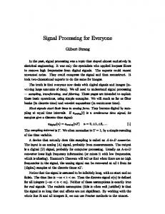
The premise for UT relies on the reflection of ultrasound at acoustic impedances, one of which is the solid propellant/gas chamber barrier. UT has two signal components. The first component sends the ultrasound into the rocket engine (or similar device) and the second component records the return signal, the reflections from acoustic impedances. The resultant signal is the subject of signal processing. Figure 1 displays the process of reflection and provides an actual recorded signal as reference. As illustrated, part of the ultrasound signal reflects at each acoustic impedance, returning to the data acquisition system to be recorded, while the rest of the signal continues through 89
Ivey, Rubenstein, Snyder, Stewart, Luebke, White, Wu, Sparks, and Whitney the medium, continuing to reflect off of other acoustic impedances.
Figure 1: Signal reflections off of acoustic impedances correlated to an ultrasound signal 3
SIGNAL PROCESSING BACKGROUND
An enlarged image of an ultrasound recording, seen in Figure 2, shows that the propellant/gas chamber echo (labeled as propellant echo) is significantly smaller than some of the other reflections. Additionally, it is not totally clear that the propellant/gas chamber echo will not be confused with noise (unlabeled data peaks). UT Data (Step Wafer Motor Configuration) adaptor + boot + propellant Settings: Meas. Freq. 0.64 MHz, Gain: 48, Output Control: 5, 3
4
FOURIER ANALYSIS
Filtering is the typical Fourier analysis method for reducing noise. Filtering refers to a process by which unwanted data, or variations, are removed from a signal. Due to the nature of the UT signal, only finite filters were considered. Filters typically work to reduce one of two kinds of noise: high frequency or low frequency noise. High frequency noise is the noise that has a higher frequency than the primary content of the signal (the echoes), and low frequency noise has a lower frequency than the primary content of the signal. The UT signal contains both types of noise. Applying standard Matlab filters [1] resulted in improved signals; however traditional filters are insufficient for UT analysis. Traditional filters do not account for the non-stationary behavior of the signal and apply the same filter to the entire signal. The ideal filter should have a high threshold (remove more noise) in the beginning of the signal and be more sensitive (remove less noise) toward the end of the signal, because later echoes are more closely related to the noise. Furthermore, traditional Fourier filters remove data based just on frequency content. The UT echoes are identified not only by frequency content, but also by amplitude. Wavelet analysis better accounts for time dependent content and captures amplitude variations better than Fourier filters. Therefore, wavelets are a better match for UT signal processing than finite Fourier filters. 5
WAVELET ANALYSIS
pulse signal
2
boot echo #1
1
propellant echo #2
boot echo #2
0 propellant echo #1
-1 adaptor echo #2
-2 adaptor echo #1
-3 0
0.00005
0.0001
0.00015
Time (sec)
Figure 2: UT signal with labeled data peaks The propellant/gas chamber edge is not the only interface where the local acoustic impedance changes. Noise, random disturbances in the signal, must also be mitigated in order to identify reflections. The signal processing algorithm applied to the ultrasound (the signal) used to calculate the web thickness has to distinguish between multiple reflections, as well as, noise to ultimately calculate the burn rate. The UT signal is finite; it has a defined time period over which the signal exists. The UT signal is nonstationary due to non-constant variance within the signal over time (the amplitude of the echoes is decreasing with time). 90
As inabilities were discovered in the Fourier analysis, solutions were found in wavelet analysis. “The traditional method of signal analysis is based on Fourier transforms, but wavelet analysis can be used where Fourier doesn’t work very well: on non-stationary data” [2]. To understand the fundamentals of wavelet analysis, consider the method by which wavelet analysis is applied to a signal. First the signal is broken into small pieces. Each small piece of the signal is then compared to a standard signal, the wavelet, and the similarities of the two signals (the small piece and the wavelet) are recorded as coefficients. Coefficients are calculated and stored for all pieces of the signal. Finally, the size of the pieces is changed and the process is repeated. The resulting outcome of wavelet analysis is a function of scale and position (time). The outcome of Fourier analysis, filtering, is a function of sinusoids. By analyzing individual pieces of the signal, wavelet analysis allow short pieces of signals to maintain significance; whereas, Fourier analysis loses time (localization) coordinate and frequency meaning [2]. The most important pieces of the UT signal are the spikes, since they represent changes in acoustic impedance. Relative to the entire signal the
Ivey, Rubenstein, Snyder, Stewart, Luebke, White, Wu, Sparks, and Whitney spikes are a small piece of the UT signal; therefore, it is critical to use an analysis that maintains the significance of individual pieces of the signal. The two important applications of wavelet analysis are shown in Figure 3. The concept of wavelet analysis is to break a signal down into approximations (a1) and details (d1). The scale is changed and the approximations are then broken down into the next level of approximation (a2) and details (d2). This cycle continues to a preset level. The resultant representation of a signal consists of the final level of approximation plus all of the levels of detail to create a lossless transformation. signal lowpass
highpass filters
Approximation (a)
Details (d)
Figure 3: Wavelet analysis representation [2] A lowpass filter allows low frequencies to pass. A highpass filter allows high frequencies through. Low frequencies change slower with respect to time than high frequencies. Therefore, in the context of wavelet approximations and details, the approximations are synonymous to low frequency content and can be thought of as a lowpass filter and the details are synonymous to high frequency content, or a highpass filter. Applying the concepts of Wavelet analysis to UT signal processing produces two important insights. First, the significant portions of the UT signal can be localized by converging on the peaks through increasingly smaller approximations. Second, filtering can be frequency dependant. The filter can sort out frequency information based both on the actual frequency of the content and based on the time position which is varied through the scale. There are two problems with wavelet analysis. The first is that the analysis is somewhat difficult to understand. There is no rule for choosing wavelets, which makes it difficult to justify the choice of one method over another. Secondly, wavelet analysis works by taking averages. However, averages may inhibit the ability to develop UT to the desired precision. Fortunately a new algorithm, Reverse High Dynamic Range Compression (RHDRC), combines the positives of wavelet analysis: localization and non-linear filtering, but lacks the limitations of wavelet analysis.
6
REVERSE HIGH DYNAMIC RANGE COMPRESSION (RHDRC)
Following the discovery of the limitations of wavelet analysis, the reverse of a high dynamic range compression algorithm (HDRC), thus RHDRC, was investigated. HDRC lowers the variance of the signal by decreasing higher rates of change (derivatives) more than lower rates of changes. The signal that results from HDRC will have more consistent amplitudes. Reversing the HDRC algorithm involves changing two aspects of the process. The derivative of a signal has less variance than the actual signal. Since RHDRC is attempting to increase the variance of the amplitudes, RHDRC should not take the derivative of the signal. Also, RHDRC should apply a nonlinear transform that serves to increase higher amplitude proportionally more than it increases lower amplitudes, the opposite of HDRC. Taking an integral nonlinearly increases the variance as long as the data points are positively correlated. The UT signal is positively correlated; previous data points are helpful in predicting future data points since the data follows a sinusoidal pattern. A point-wise integration of the data, while it is a nonlinear transformation, does not capture frequency meaning, but integration of semi-waves does capture frequency content. Integration of semiwaves, using discrete data, involves the summation of all data points until the signal crosses zero. The actual algorithm works by tracking the current coefficient of the data (positive or negative) and summing all data until the sign changes. The semi-wave integration is a nonlinear function of both frequency and amplitude. The examination of both components will lead to the fundamental understanding of the power behind a fairly basic concept. First consider the frequency component. Assume that two waves have the same amplitude, but wave 1 has a greater frequency than wave 2. Since frequency is inversely related to period, wave 1 has a shorter period than wave 2. Thus, the semi-wave of wave 1 is shorter than the semi-wave of wave 2, so the area under semi-wave 1 is less than the area under semi-wave 2. Therefore, the value of the semiwave integration is proportionally less for higher frequency content than lower frequency content. The second component of the nonlinear function is amplitude. The mean of a semi-wave with higher amplitude will be higher than the mean of semi-wave with lower amplitude, given that the waveforms are comparable (the shape of the waves is similar). Assuming that both waves have the same frequency, the one with the higher mean value, the higher amplitude, will have a greater area. Therefore, the semi-wave integration will be greater for the semi-waves with the higher amplitude.
91
Ivey, Rubenstein, Snyder, Stewart, Luebke, White, Wu, Sparks, and Whitney The frequency is inversely proportional to the value of the semi-wave integration and amplitude is directly proportional. Therefore, semi-wave integration is highest for low frequency, high amplitude content. Recall that the ideal algorithm should extract the echoes from the UT signal. The echoes are primarily distinguished as having higher amplitudes than the rest of the signal. The most prominent noise in the UT signal is high frequency. Even though there is low frequency noise, the noise is close enough to zero that the high frequency noise can distort the low frequencies to cross zero; leading to the conclusion that high frequency noise is the dominant type of noise in the signal. Therefore, semi-wave integration proportionally increases the echoes more than any other part of the signal through components, frequency and amplitude. Semi-wave integration results in the calculation of a single value for each semi-wave; therefore, semi-wave integration is not a lossless transformation. The original signal cannot be reconstructed from the semi-wave integration values. For UT signal processing, however, it is sufficient to represent a semi-wave by just one data point, the semi-wave integration value. The final choice in how to implement semi-wave integration is where to locate, with respect to time, the single representative semi-wave integration value. Because of the stability of the median value, the value of semiwave integration is assigned the time value of the semiwave median. The final outcome of reversing HDRC is an algorithm that follows a two-step process: 1.) Calculate the semi-wave integration. The semi-wave integration is calculated by adding all amplitudes together until the sign of the amplitude changes. The value of the integral of each semi-wave, an amplitude value, is assigned the median time value of the semi-wave. Thus, each semi-wave is represented by a single amplitude and time value. 2.) Threshold the representative point of each semi-wave (the result of step 1). The threshold is set just below the value of the highest amplitude of the smallest echo that should remain in the signal. All points below the threshold are set equal to zero. By using a threshold, the signal is reduced to include only the meaningful content. The original signal contains around 25,000 data points. The reduced signal contains around 250 data points. Clustering is a formal mathematical routine for identifying groups of data points. The reduction in size of the signal allows clustering to become a viable option for formally grouping/identifying the waves within each signal. Clustering algorithms require a distance matrix, the distance from every point to every other point, as input. The size of the distance matrix is the square of the number of points to be clustered, thus limiting clustering applications to smaller data sets. 92
The result of clustering is a set of distinct groups. The groups are interpreted as different wavefronts, or echoes. The wavefronts, for comparison purposes are identified by the median value of the wavefront for the same reason that the median in used for the integrals. Using the same algorithm (particularly the same threshold) on all signals, the number of wavefronts should be equal across all signals. The UT system records signals on a constant time interval. By differencing the time occurrence of wavefronts between files, the distance that each wave moves with respect to time is calculated. By multiplying by the speed of sound, the wavefront movement is converted into a distance movement. Finally the burn rate, the rate of change of height with respect to time has been calculated. 7
CONDITION-BASED ANALYSIS
The precision of the algorithm is dependent on the data, the signal that it is processing. There are certain aspects of the signal that an effective algorithm should leverage, including: frequency, amplitude and time dependence. There is also information that is not contained within a single signal that the ideal algorithm should leverage as well. What allows a viewer to identify the propellant/gas chamber barrier is the fact that the echo from that barrier moves across files, with respect to time. The ideal algorithm should leverage the information that the desired echo is moving with time, similar to the way that an eyeball approximation would be performed. The condition based analysis will look at each condition that can be leveraged and analyze how RHDRC performs within each category. RHDRC takes advantage of the frequency meaning of the signal by proportionally creating a greater semiwave integration value for low frequency content than high frequency content. Low frequency content has a semi-wave integration value x times greater than the high frequency content, where x represents the proportion of the frequencies (high frequency divided by low frequency). RHDRC properly takes advantage of the frequency component, because the echoes are expected to be lower frequency than the noise. Since there is no limit to the proportion that frequency differences could be scaled, the ideal algorithm needs to simply provide a logical scaling component. The frequency content is not the only component that the algorithm needs to leverage. Since there is no reason to leverage frequency more than amplitude, both should be leveraged the same (and they are by RHDRC). Furthermore, the integral provides a logical interpretation whereas further scaling does not have as intuitive of an explanation. The amplitude of the echoes tend to be greater than the noise. The semi-wave integration value is x times
Ivey, Rubenstein, Snyder, Stewart, Luebke, White, Wu, Sparks, and Whitney greater for a higher amplitude semi-waves where x is the proportional difference in amplitude (larger average amplitude divided by lower average amplitude). RHDRC scales the echoes proportionally more than the noise, making the echoes easier to identify. Scaling by the proportion of the amplitude difference has a logical interpretation and provides the same weight to amplitude as frequency. Time dependency refers to the location of the data point along the signal. The UT signals are non-stationary with the echoes decreasing in amplitude with time. The ideal algorithm should take this information into account by being more sensitive at the end of signals as the echoes become closer in amplitude to noise. The current RHDRC algorithm does not account for time dependency. Simply by decreasing the threshold as time increases, RHDRC would account for the time dependent component. Therefore, while the current version of RHDRC does not account for the time component, the algorithm could be easily modified if time dependency ever becomes significantly important to the analysis. The final component involves the movement of wavefronts across files. RHDRC does not leverage the movement across files, but allows the user to perform this analysis. It is known that across files, or with respect to time, that the propellant/gas chamber wavefront is moving. RHDRC calculates burn rate by comparing the representative point of each wave across files. Therefore, the burn rate calculation captures the information about the movement across files. If the user wants to leverage this information, the user can perform a linear regression that will smooth the data. Since it is relatively easy to perform a linear regression that is similar to the method that RHDRC would use to leverage the file component information (predicting the next wavefront location by the past values) the decision is left to the user whether to perform this analysis. 8
QUANTITATIVE RESULTS
Testing of the UT system and the RHDRC algorithm was performed on a mock rocket engine. The mock engine consisted of a non-metallic boot and water in place of solid rocket propellant. The water is leaked out of the system. A digital scale recorded the weight of the system every 0.2 seconds. Calibrations allow the weight data to be transformed into water height measurements with respect to time, thus serving as the comparison for the UT flow rate measurements. Four experiments, each with ten trials were performed. The experiments varied the ultrasonic power and the medium (water was replaced with milk). The results in Table 1 are representative of the testing results. Experiment 1, trials 5-14 (excluding 6th trial)
Mean 0.937818618% Variance 4.312262543% Standard Deviation 2.076598792% Table 1: Percent error, (weight flow rate minus UT flow rate; divided by weight flow rate). Trial 6 was excluded because the height residuals from the scale data from the linear regression exhibited a distinct pattern. However, the residuals from the UT data did not exhibit a similar pattern. The weight data from trial 6 was assumed corrupt and not included in the experiment. The mean percent error is less than the 1% requested for a non-metallic boot in the initial statement of work. The residuals from the linear regression for the UT flow rate, showed a pattern of higher variance at the beginning of the data, followed by lower variance. While nonconstant variance normally invalidates the regression results, in the case of the UT data these residuals suggest that the UT measurement is actually more precise than the digital scale. When the water is poured into the boot at the beginning of the experiment, ripples oscillate on the surface. Once a sufficient flow rate is established the ripples fade out. It is expected that the UT would capture such oscillations. This water experiments gave quantitative support for UT. Future testing should be performed with a more accurate independent measurement of the flow rate. 9
GRAPHICAL USER INTERFACE (GUI)
To facilitate the use of the new algorithm, a graphical user interface (GUI) was developed. The GUI was developed in Matlab 6.1 and allows the user to control all of the parameters of the algorithm through a simple point and click interface. The GUI has two primary goals. First it must be simple to use and show feedback to the user so as to keep the program from being confusing. Secondly, it must allow the user to adjust all of the parameters for the algorithm. These two goals have been achieved by status bars and forcing functions to allow the user to get a good concept of the current state of the algorithm, as well as keep the user from going through steps out of order. 10 CONCLUSION A statistical analysis of variance caused by each component is a difficult and unneeded exercise after realizing that RHDRC is not a primary source of error in the UT measurements. RHDRC leverages, or allows for easy modification to leverage, all available information available in a UT signal. Theoretically there is no other algorithm that could perform the transformation of the signal any better than RHDRC. The information contained be93
Ivey, Rubenstein, Snyder, Stewart, Luebke, White, Wu, Sparks, and Whitney tween files is incumbent in the burn rate output and can be leveraged as the user sees fit. Beyond a practical understanding of RHDRC and the conditional based analysis, actual testing has revealed that the algorithm in no way limits the performance of the UT analysis. The RHDRC algorithm was used to analyze the data collected from water tests. The RHDRC algorithm successfully identified the wavefronts across all files for all trials. Figure 4 shows the results from one of the trails. It is clear that RHDRC removes the echoes far enough from the noise that it is able to always identify the echoes so long as they are present in the signal. Toward the end of the signal secondary echoes are not easily identified but this is due to a lack of difference in the data. No algorithm can distinguish an echo from noise, when there is no available information that distinguishes the two components. From both the conditional analysis that established the performance of RHDRC within categories and from the actual use of RHDRC, the RHDRC algorithm fully satisfies the UT signal processing needs.
REFERENCES [1] Vinay K. Ingle and John G. Proakis. Digital Signal Processing using Matlab©. Pacific Grove, CA: Brooks / Cole Publishing Company, 2000. [2] Anne Mascarin, “Webinar: Wavelet Toolbox,” [Online Webinar recording] (March 20, 2002), [cited 2002 November 22], Available at HTTP: http://www.mathworks.com/programs/webex/wavelet /bounce.html BIOGRAPHIES JESSICA IVEY is a fourth year Systems Engineering major with a minor in Technology, Management, and Policy. Jessica is from Roanoke, Virginia, and when she is not developing test plans and pattern predictions for the Capstone team, you can find her hiking on the Blue Ridge parkway or kicking the soccer ball. Next year, Jessica will be working for Booz Allen Hamilton in Washington D.C. THOMAS RUBENSTEIN is a fourth year Systems Engineering Major from Pensacola, Florida. If one can tear Tom away from developing GUIs, he can be found boarding down the ski slopes. Tom will begin training to be a submariner in the US Navy this summer.
Figure 4: (Top) Original signal with minimal echoes. (Bottom) Original signal transformed through RHDRC 11 RECOMMENDATIONS Due to cost limitation testing was only performed on a simulated rocket engine with a non-metallic adaptor. Further testing should be performed using a metallic adaptor and solid propellant rocket engines, both of which will increase the noise in the UT signal. RHDRC performed without fail on the current testing data, but needs to be tested on the noisier signals. All theoretical and analytical work supports that RHDRC will perform satisfactory on the real, noisier data but the testing does need to be performed.
94
AMANDA SNYDER is a fourth year Systems Engineering Major concentrating in Management. She is from Chantilly, Virginia, and when she’s is not calculating flow rate, she likes to spend her time sunbathing in the Bahamas. Amanda is moving the New York, NY next year to work for Kurt Salmon Associates. MICHAEL STEWART is a fourth year Systems Engineering and Economics double major from Chantilly, Virginia. Michael spent the majority of the past year appreciating the merits of the Reverse High Definition Range Compression algorithm in predicting burn rate. In his free time Michael enjoys flying along the east coast, as he will soon be getting his pilot’s license. He will be working for Appian next year in Vienna, Virginia.