developing an optimization algorithm to form district ...

ΤΗΕΜΕ B: URBAN WATER MANAGEMENT

ID 117

DEVELOPING AN OPTIMIZATION ALGORITHM TO FORM DISTRICT METERED AREAS IN A WATER DISTRIBUTION SYSTEM Korkana P.1, Kanakoudis V.2, Patelis M.3, Makrysopoulos A.4, Gonelas K.5 1

Civil Engineer, Department of Civil Engineering, University of Thessaly, Pedion Areos, Volos, GR 38334, Greece, 2 [email protected]; Associate Professor, Department of Civil Engineering, University of Thessaly, Pedion Areos, Volos, GR 3 38334, Greece, [email protected]; PhD Candidate, Department of Civil Engineering, University of Thessaly, 4 Pedion Areos, Volos, GR 38334, Greece, [email protected]; Student, School of Electrical and Computer Engineering 5 National Technical University of Athens, Athens, GR 15780, Greece, [email protected]; Research Associate, Civil Engineer PhD, Department of Civil Engineering, University of Thessaly, Pedion Areos, Volos, GR 38334, Greece, [email protected]

ABSTRACT District Metered Areas (DMAs) formation is widely recognized as one of the most cost-effective methods towards optimal water distribution network (WDN) management. It is also a prerequisite for more sophisticated water loss reduction techniques applied. Forming optimal sized DMAs by placing the necessary isolation valves, is not an easy task to do. The present paper presents the process of developing an optimization algorithm to form DMAs in a WDN. Exploiting the numerous possibilities resulting from the inter-connection of Matlab and Epanet (WDN simulation) software, an algorithm (code) is produced in C++ language. The code reads all the significant data of the WDN resulting from Epanet. Matlab defines the optimal sites to place the necessary isolation valves in terms of water losses reduction, considering vital limitations in order the WDN to operate properly. This code can be applied in any WDN case. The outcome is a hierarchical list of pipes to be closed (via placing isolation valves) forming DMAs. The hierarchical criterion used is the higher reduction in the network’s operating pressure. Keywords: optimization, DMAs, water loss

1. INTRODUCTION District Metered Areas (DMAs) formation is widely recognized as one of the most cost- effective methods towards optimal Water Distribution Network management (WDNs) [1]. It is also a prerequisite for more sophisticated water loss reduction techniques applied. Sectorization of a network results in several significant benefits [2], [3] such as increased system control and contributes to the mitigation of water losses. Implementation of a DMAs’ formation project can be carried out under several perspectives with different goals each time. Moreover, in real cases achieving the optimal design of DMAs may be a very challenging task due to the intrinsic complexity of the WDNs, as presented in many examples of DMAs formation up to date [4], [5], [6]. Therefore, development of a methodology able to provide support to water utility managers (decision-makers) is required. In recent years, an increasing number of researches have addressed this problem and various optimization approaches can be found in literature [7], [8]. Some of the techniques developed so far suffer from limitations and drawbacks, which are mainly based on the limited number of DMAs’ design criteria and the dependence on the size of the WDN [9]. With the inter-connection of Matlab and Epanet [10], there is the possibility to produce a code that collects data from the network and provides results, as well as, codes that run tests on the WDN. Combination of these two software tools, forms an expert tool that can be used to optimize the network’s segmentation into DMAs. In the study presented in this paper, two codes in C++ language are

nd

2 EWaS International Conference, 1- 4 June, 2016 - Chania, Crete, Greece.

ΤΗΕΜΕ B: URBAN WATER MANAGEMENT

ID 117

developed in order to satisfy two separate but relevant objective functions. The first code collects data from the WDN, to “feed” its simulation model developed through EPANET, and perform certain calculations. The second code uses a preprogrammed tool named “combinator”, to produce all the different possible combinations of closed pipes (simulating the locations where isolation valves could be placed). Each combination is then being tested on the WDN’s hydraulic simulation model. Finally, data from each combination being tested is collected and evaluated. Evaluation of data, determines whether a combination is an optimal solution or not. The codes take into account several rules on DMA’s formation. In more detail, nodal pressure variation, fire flow requirements, water mains, population density, network’s topology and minimum pressure requirements determine DMAs’ borders. DMAs optimal formation aims to reduce the total (sum) nodal pressure as much as possible. A number of pipes are selected to be closed placing isolation valves. The entire process is being tested on a dummy case study WDN.

2. ALGORITHM/CODE No1: DATA COLLECTION An optimization process has to have a universal character and be able to be used in any WDN. A short separate code is written, in order to identify the case study WDN. This code is written in C++ language and its purpose is to connect Matlab with EPANET as well as collect certain data from the network. Matlab is used for codes programming. On the other hand, Epanet performs hydraulic simulation of the case study WDN. Hourly nodal demand and pressure values are collected, and equation (1) is being calculated, where, i is a custom node of the network, Di,t is demand of node i for each time step t [lt/sec], and Pi,t is pressure of node i for each time step t [KPa]. 𝑃𝐷 = ∑ni=1(Pix Di )

(1)

CODE No1: DATA COLLECTION [errcode]=ENopenH();%OPEN HYDRAULICS ANALYSIS [errcode]=ENinitH(1);%INITIALIZE TIME TO 1 k=1; [errcode,step]=ENnextH(); while (step>0 && errcode==0); [errcode,t]=ENrunH(); [errcode,step]=ENnextH(); for i=2:81 ;% for all the 80 nodes [errcode,pressure(k,i)]=ENgetnodevalue(i,11); %%PRESSURE=11 [errcode,demand(k,i)]=ENgetnodevalue(i,9);%% DEMAND=9 pd(k,i)=pressure(k,i)*demand(k,i); end k=k+1;%increase time step for Pressure vector. end sum(sum(pd)) [errcode]=ENcloseH(); %close hydraulic analysis

As Epanet cannot perform pressure driven analysis (i.e. pressure dependent nodal consumption), the nodal water demand is considered to be only volume dependent. This code aims only at identifying the network and does not perform any optimization process.

3. ALGORITHM/CODE No2: OPTIMAL SELECTION OF PIPES TO BE CLOSED

nd

2 EWaS International Conference, 1- 4 June, 2016 - Chania, Crete, Greece.

ΤΗΕΜΕ B: URBAN WATER MANAGEMENT

ID 117

Optimization of forming DMAs procedure is based on the philosophy of exploiting every possible combination of closed pipes, in order to select which ones provide better pressure management results. Thus, in the current study, a second code is developed in C++ programming language. This code uses a preprogrammed tool (named “combinator”) to produce every possible combination of closed pipes in the case study network. After counting all network pipes, the program closes one pipe and tests the resulting pressure management (reduction) impact. Each pipe is being tested alone and the one that reduces the most the “P*D” product is chosen as a pipe to be permanently closed (i.e. site to place an isolation valve). Then keeping the previous pipe closed, the code checks all remaining pipes and finally closes the one that reduces the most the “P*D” product again. This stepwise procedure is continued till the optimal number of closed pipes is determined, providing in that way a hierarchical list of sites where isolation valves should be placed. It is obvious that after defining the optimal number of closed pipes, every new closed pipe will not reduce any further the product ‘’P*D’’ using equation (1). Although this optimization process might demand great computational power, it has the ability to give in return a safe optimal solution. As already stated, the great disadvantage of this optimization process is that it requires a lot of computational time to test each different combination (scenario) of closed pipes. In order to reduce the time needed and make things easier for the program, certain pipes are being pre-excluded from the process. For example, pipes delivering water to ending nodes cannot be part of the process, as, if they were closed, then water would never reach the ending nodes. Also water mains and other pipes delivering significant water volumes can also be excluded from the optimization process. Based on the above, many pipes are removed from the pipe list of the program. Thus, combinations needing to be tested are considerably reduced and calculation time is significantly reduced. Reduction of tested pipes depends on the morphology of the network being studied and may not apply to every case with the same extent. A group of pipes has to fulfil some prerequisites in order to be accepted as a potential optimal solution of the optimization process. A closed pipe should not result in negative pressures at any node of the network. In Epanet, negative pressure occurs when water does not reach one or more nodes. Additionally, as set by the Greek legislation, the nodal pressure in every water network has to be maintained above a minimum requirement of 29 psi (200kPa). CODE No2: OPTIMAL SELECTION OF PIPES TO BE CLOSED p1=combinator(m,1,'c');%sunduasmoi agvgvn ana 1 c=size(p1,1); pressure=[0 0]; .... for h=1:m; s=0; s1=0; if h>1; clear z; xc=size(B,2); for i=1:xc-1 if B(i)B(xc); s1=s1+1; end end if s>0; N(h-1)=x1(B(xc)-s); nd

2 EWaS International Conference, 1- 4 June, 2016 - Chania, Crete, Greece.

ΤΗΕΜΕ B: URBAN WATER MANAGEMENT x1(B(xc)-s)=[]; elseif s1==xc-1 N(h-1)=x1(B(xc)); x1(B(xc))=[]; else N(h-1)=x1(B(xc)-(xc-1)); x1(B(xc)-(xc-1))=[]; end c=size(x1,2); disp(x1) disp(N) end for j=1:c; [errcode]=ENinitH(1);%INITIALIZE TIME TO 1 if h>1; for i=1:h-1 %Kleinei tous agwgous pou vrhkame oti prepei n einai kleistoi [errcode]=ENsetlinkvalue(pipeIndex(N(i)), 11, 0); end end k=1; if h>1 [errcode]=ENsetlinkvalue(pipeIndex(x1(j)), 11, 0); else [errcode]=ENsetlinkvalue(pipeIndex(p1(j,1)), 11, 0); end if h>1 z(2,j)=x1(j);%APOTHIKEYOYME TO ONOMA TWN KLEISTWN AGWGWN else z(2,j)=p1(j,1); end [errcode,step]=ENnextH(); while (step>0 && errcode==0); [errcode,t]=ENrunH(); [errcode,step]=ENnextH(); for i=2:81 ;% for all the 9 nodes bf=false; [errcode,pressure(k,i)]=ENgetnodevalue(i,11);%%PRESSURE=11 [errcode,demand(k,i)]=ENgetnodevalue(i,9);%% DEMAND=9 pd(k,i)=pressure(k,i)*demand(k,i); if pressure(k,i)4999999; q=q+1; end end if q==c; break end r=find(A==(min(A))); for i=1:1 v(h)=r(i); end g(h)=z(1,v(h)); B(h)=z(2,v(h));

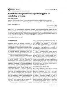
4. THE CASE STUDY NETWORK Both codes are being tested on a case study (dummy) network chosen that consists of one reservoir supplying water to the entire network through 100 pipes, two boosters assuring the required hydraulic pressure, as well as a water tank to store water and supply it back to the network (Figure 1). Size and complexity of this network is not great, however is enough to resemble the case of any small town, or a part of it. The specific case study network is based on Bentley’s WaterGems simulation software lessons library and is a verified and calibrated example of a real case, unknown though, network. The objective of the study is to divide the network into a proper number of DMAs, so that the maximum control of pressure is achieved. It is proven that most of the times forming DMAs does not only offer better control of the network and better observation of its performance, but it also achieves a small but significant decrease in the overall operating pressure level of the network even if no PRVs are installed, as the water flowing through the network pipes is forced to follow specific more “energy consuming” paths. DMA forming in the field takes place by installing isolation valves. In this study though, instead of installing such valves, the initial operating status of a pipe is defined as closed or open.

Figure 1. The case study network 5. OPTIMIZATION AND RESULTS

nd

2 EWaS International Conference, 1- 4 June, 2016 - Chania, Crete, Greece.

ΤΗΕΜΕ B: URBAN WATER MANAGEMENT

ID 117

Regarding the optimization process, in order to calculate the “P*D” product according to equation (1), code No1 is used first. This was performed as described above in order to identify the network being studied and measure its nodal pressure level. The initial “P*D” product was calculated at 1,569,900 psi*gallons. Before using the code No2, a thorough observation of the network took place. As mentioned before, several pipes could be excluded from the second code’s tests as they were not potential optimal solutions. Thus, 20 pipes (i.e. P-1, P-2, P-3, P-4, P-5, P-6, P-7, P-9, P-10, P11, P-18, P-241, P-242, P-247, P-248, P-250, P-251, P-252, P-253 and P-259) were left out (that is 20% of the total number of network pipes), significantly reducing the number of combinations to be tested and computational time needed. This pipe exclusion process has to be decided by an expert with good understanding of the network being studied. The number of excluded pipes may significantly differ from one case to another, but is a standard procedure for the optimization process. The second phase of the study was to start the optimization process on the case study network. Code No2 was applied step by step, meaning that it was only used to find one optimal closed pipe each time. In this way the test results could be better monitored and controlled. After several tests and trials, the program was ready to work alone and perform the optimization process. Numerous combinations were tested in order the program to reach a certain result and specifically address which pipes should be closed. The pipes that were chosen to close were 8 (i.e. P-17, P-36, P-90, P-229, P-93, P-254, P-232, P-240) out of the 80 left (Figure 2). It is very important to mention that the code performing the optimization process is able to reveal the impact of each pipe being successively closed. As the optimization process evolves, according to the pattern explained above, not every closed pipe reduces the product ‘’P*D’’ the way. It can be easily understood from Τable 1, that every closed pipe reduces product ‘’P*D’’ less than the previous one. The value of this observation is that in cases of limited budget for such a project (DMA forming), this program is able to pinpoint and hierarchical analyze the most significant interventions. The program gradually reaches the optimal DMAs formation. In the case study network selected four different DMAs were formed (Figure 2).

Figure 2. Closed pipes shown with a light green line & DMAs’ formation

nd

2 EWaS International Conference, 1- 4 June, 2016 - Chania, Crete, Greece.

ΤΗΕΜΕ B: URBAN WATER MANAGEMENT

ID 117

This process showed that the best (optimal) scenario of placing isolation valves to form DMAs is to successively close no more than eight network pipes (Table 1). Figure 3 demonstrates the “P*D” reduction resulting from the abovementioned stepwise optimization process for the optimal scenario. There are two alternative scenarios of eight pipes being closed (Scenario A: P-17, P-36, P-90, P-229, P-93, P-254, P-232, P-240; Scenario B: Ρ-231, Ρ258, Ρ-256 Ρ-146, Ρ-262, Ρ-227) that result in the same maximum “P*D” reduction that reached 13.64% compared to the initial status (no pipe closed). Thus, these two scenarios are considered “equivalent”. The fact that the second code did continue the optimization process for another six pipes being successively closed, was left out as ‘’P*D’’ was reduced by less than 0.1% for each one pipe being closed after the eighth one. So, these additional six pipes were left open as the water utility manager/decision maker should always consider how feasible and realistic the suggested project is, regarding its implementation. Also, these six pipes are not important for the DMAs formation as they do not offer any changes to DMAs’ borders.

Table 1. Closed pipes’ hierarchical list along with the new calculated product ‘’P*D’’.

Pipes (Numbered in code) 7 7,12 7,12,21 7,12,21,38 7,12,21,38,22 7,12,21,38,22,50 7,12,21,38,22,50,41 7,12,21,38,22,50,41,48

Pipes (Name in EPANET) P-17 P-17, P-36 P-17, P-36, P-90 P-17, P-36, P-90, P-229 P-17, P-36, P-90, P-229, P-93 P-17, P-36, P-90, P-229, P-93, P-254 P-17, P-36, P-90, P-229, P-93, P-254, P-232 P-17, P-36, P-90, P-229, P-93, P-254, P-232, P-240

P*D (psi * gallons) 1,466,400 1,390,600 1,360,700 1,359,000 1,357,400 1,357,200 1,357,000 1,355,800

PD additional reduction resulting for each succesive step of the optimization process

1.470.000

P*D (psi * glns)

1.450.000 1.430.000 1.410.000 1.390.000 1.370.000 1.350.000

Pipes being successivelly closed Figure 3. “P*D” reduction resulting from each additional pipe being closed The goal to define the optimal borders of DMAs was achieved. This optimization process could be used to solve the same problem on different water networks. Its main disadvantage though is that it depends a lot on the size of the case study network. As the number of pipes increases, the complexity of the problem increases too and more combinations have to be tested. This may need too much computational power nd

2 EWaS International Conference, 1- 4 June, 2016 - Chania, Crete, Greece.

ΤΗΕΜΕ B: URBAN WATER MANAGEMENT

ID 117

and time. If the number of combinations were reduced in some way, then this optimization process would become more applicable. It can be used though is relatively small networks. One more disadvantage of the process is that code No2 provides only a group of closed pipes. Some of these pipes may define DMAs borders, but some others may not. This has to be figured out by studying the network, after pointing out which pipes are closed. Optimization of DMAs forming process is based on two codes developed that select the group of pipes to be closed. Through the selection of those pipes, guidance is offered to design DMAs’ borders. The codes may have been developed to define the optimal DMAs formation of a network by reducing pressure as much as possible but, DMAs implementation is also used for various purposes (i.e. network monitoring; better network performance; perquisite for other more sophisticated pressure management measures implementation). The optimal solution resulting from this process was indeed verified. Closed pipes did not produce any negative nodal pressure and pressure level in the network did not fall below 200Kpa (29 psi). DMAs’ borders may differ, if other pressure management implementations have to be considered too. Not all closed pipes also define DMAs’ borders. PD reduction percentage is only a characteristic figure of pressure control resulting from isolating a certain group of pipes. It does not represent any expectation on pressure reduction at network scale. Since this study is not based on pressure driven analysis, nodal pressure and demand after DMAs formation may differ. If pressure reduction at network scale is achieved due to forming DMAs, a change of its input volume is expected too.

6. CONCLUSIONS Matlab and EPANET combined, produced an accurate optimization tool to define the optimal borders of DMAs. Two codes in C++ were developed to connect Epanet with Matlab and perform the optimization process. Results came out after checking every combination of closed pipes in a case study network of 100 pipes. Optimal DMAs’ formation resulted after closing just 8 pipes although the program went on closing additionally 6. Use of this program showed that a C++ code is able to identify every network and optimize its division to several DMAs. The criterion used to define the optimal solution was the reduction of total “P*D” at network scale. The codes rejected any potentially closed pipe that would lead to operational problems and suggested one group of pipes that fulfilled the minimum nodal pressure requirement (≥ 200kpa). Results were separately verified. Although this optimal solution resulted in pressure reduction, this was not “interpreted” to water losses savings and even excessive water demand reduction since the analysis applied was not pressure driven (nodal water demand was not considered pressure dependent as it actually is). In order to reduce the numerous tests of closed pipes combinations, several pipes were preexcluded from the entire process. These pipes were thoroughly examined and excluded since they cannot actually represent a possible solution to the problem. Although this pre-exclusion process significantly reduced the computation power and time needs, both still represent the main disadvantage of the optimization process. DMAs formation using this optimization process can be applied in any water distribution network. The case study selected was a network with real characteristics but limited number of pipes and devices. Bigger networks will demand more time and further calibration in order to be used by the codes developed. Although EPANET is free, easy to use software, Matlab on the contrary, demands C++ programming knowledge in order to develop codes and apply them. The optimization tool developed is able to provide reliable results but can be further studied and enriched in order to provide other important information as well as reduce the required processing power and time.

nd

2 EWaS International Conference, 1- 4 June, 2016 - Chania, Crete, Greece.

ΤΗΕΜΕ B: URBAN WATER MANAGEMENT

ID 117

Acknowledgements This work is elaborated through a project co-funded by the European Union, IPA Adriatic CBC Programme 20072013 (DRINKADRIA project, 1o str./0004, further info: www.drinkadria.eu). References 1. Kanakoudis V., Gonelas K., 2014. Applying Pressure Management to Reduce Water Losses in Two Greek Cities’ WDSs: Expectations, Problems, Results and Revisions, Procedia Engineering, 89(2014), 318-325 2. Savić D., Ferrari G., 2015. Economic Performance of DMAs in Water Distribution Systems, Procedia Engineering, 119(2015), 189–195 3. Gonelas K., Kanakoudis V., 2015. The economic impact of Pressure Management in Kozani City’s Water Distribution System. Benefits, expenditures and revenue losses, Conference Paper, IWA Balkan Young Water Professionals 2015, (1),182-190 4. Charalambous B., 2005. Experience in DMA redesign at water board of Lemesos, Cyprus, Proceedings of the IWA Specialized Conference Leakage 2005, Halifax, Nova Scotia, Canada. 5. MacDonald G., Yates C., 2005. DMA design and implementation, an American context, Proceedings of the IWA Specialized Conference Leakage 2005, Halifax, Nova Scotia, Canada. 6. Rogers D., Reducing leakage in Jakarta, Indonesia, 2005. Proceedings of the IWA Specialized Conference Leakage2005, Halifax, Nova Scotia, Canada. 7. Abraham E., Parpas P., Stoianov I., 2015. Control of water distribution networks with dynamic DMA topology using strictly feasible sequential convex programming. Research Article from AGU Publictions, Water Resources Research, December 2015. 8. Araujo L., Ramos H., Coelho S., 2006. Pressure Control for Leakage minimization in Water Distribution Systems Management, Water Resources Management, 20(1), 133-149 9. Galdiero E., 2015, Multi-Objective Design of District Metered Areas in Water Distribution Networks, Thesis submitted for the degree of PhD in Hydraulic and Environmental Engineering, Dipartmento di Ingegneria Civile, Edile ed AMbientale, Naples 2015 10.Eliades G., Kyriakou M., Polcarpou M., 2014. Sensor placement in water distribution systems using SPLACE Toolkit. Procedia Engineering 70:602-611, 2014

nd

2 EWaS International Conference, 1- 4 June, 2016 - Chania, Crete, Greece.