TECHNICAL PAPER
ISSN:1047-3289 J. Air & Waste Manage. Assoc. 58:1360 –1369 DOI:10.3155/1047-3289.58.10.1360 Copyright 2008 Air & Waste Management Association
Developing and Evaluating Techniques for Localizing Pollutant Emission Sources with Open-Path Fourier Transform Infrared Measurements and Wind Data Chang-Fu Wu Department of Public Health and Institute of Occupational Medicine and Industrial Hygiene, National Taiwan University, Taipei, Taiwan, Republic of China Ching-Hui Chen and Shih-Ying Chang Institute of Occupational Medicine and Industrial Hygiene, Institute of Environmental Health, National Taiwan University, Taipei, Taiwan, Republic of China Pao-Erh Chang, Ruei-Hou Shie, Lung-Yu Sung, Jen-Chih Yang, and Jen-Wei Su Industrial Technology Research Institute, Hsin-chu, Taiwan, Republic of China
ABSTRACT This paper presents the simulation and field evaluation results of two approaches to localize pollutant emission sources with open-path Fourier transform infrared (OPFTIR) spectroscopy. The first approach combined the plume’s peak location information reconstructed from the Smooth Basis Function Minimization (SBFM) algorithm and the wind direction data to calculate source projection lines. In the second approach, the plume’s peak location was determined with the Monte Carlo methodology by randomly sampling within the beam segment having the largest path-integrated concentration. We first conducted a series of simulation studies to investigate the sensitivity of using different basis functions in the SBFM algorithm. It was found that fitting with the beta and Weibull basis functions generally gave better estimates of the peak locations than with the normal basis function when the plumes were mainly within the OP-FTIR’s monitoring line. However, for plumes that were symmetric to the peak position or spread over the OP-FTIR, fitting with the normal basis function gave better performance. In the field experiment, two tracer gases were released simultaneously from two locations and the OP-FTIR collected data downwind from the sources with a maximum beam path length of 97 m. For the first approach, the release locations were within the 0.25- to
IMPLICATIONS The two techniques evaluated in this study may provide near real-time location estimates of air pollutant emissions. Because the OP-FTIR can scan over a long distance, these techniques are most useful for monitoring large spatial areas (e.g., near industrial complexes or hazardous waste sites). One could apply these techniques as screening tools to narrow down the potential areas in which to search for the source(s) and then use conventional tools, such as photoionization detectors, to conduct a detailed survey.
1360 Journal of the Air & Waste Management Association
0.5-probability area only after the uncertainty of the peak locations was included in the calculation process. The second approach was easy to implement and still performed as satisfactorily as the first approach. The distances from the sources to the best-fit lines (i.e., the regression lines) of the estimated locations were smaller than 10 m. INTRODUCTION Localizing (i.e., locating) toxic air pollutant sources is an important issue in many environment and health-related fields. To minimize the air pollutants’ impact on the environment and the public health, it is necessary to identify the releasing sources in a timely fashion so that an effective control strategy can be implemented. For example, in homeland security applications, the release locations of harmful airborne contaminants usually are unknown. Their locations must be estimated from the postrelease concentration observations.1 Another example is the leak detection of volatile organic compounds (VOCs) from the refinery or petrochemical industries. Detecting the source of a leak from thousands of possible components is always a challenging task; nevertheless, fixing the identified leaking components not only protects public health and the environment but also reduces waste and any potential liability. For a large area, one way to locate the fugitive emission source(s) of hazardous chemicals is placing a matrix of point samplers at the monitoring site. In Chen et al.,2,3 3-hr canister samples were taken from 25 sites inside a petrochemical plant, twice per season for 1 yr. These samples were then analyzed with gas chromatography/ mass spectrometry (GC/MS) according to the U.S. Environmental Protection Agency (EPA) TO-14 method. A total of 19 emission sources were located from the contour maps of the VOC measurements. However, these point samplers provide only time-integrated information and the whole sampling and analysis process is rather time consuming. For example, a complete VOC monitoring Volume 58 October 2008
Wu et al. campaign with canisters may take more than 1 week, including canister cleaning, sampling, GC/MS analysis, and data processing.2 Although there are currently several in situ monitoring devices (such as electrochemical sensors) that can provide real-time information about the concentrations of airborne chemicals, they usually can only monitor certain chemicals. Each chemical needs a specific type of detector. In other words, prior knowledge about the properties of the chemical to be detected is required. Several researchers use open-path Fourier transform infrared (OP-FTIR) spectroscopy to overcome some of the limitations above. The OP-FTIR can identify and quantify multiple air pollutants and provide real-time information in situ.4 When scanning two-dimensionally across the monitoring areas, OP-FTIR covers a much larger area than the point samplers to obtain spatially representative data. The hot spots or high concentration regions could further be identified by reconstructing concentration maps from the OP-FTIR’s path-integrated concentration (PIC) data with computed tomography (e.g., refs 5 and 6), or radial plume mapping techniques (e.g., refs 7 and 8). In situations when the above two-dimensional scanning geometry is not feasible to set up, one can also deploy the OP-FTIR in a one-dimensional (1D) fashion at a downwind location. Combining the OP-FTIR’s PIC data and wind direction information, we can estimate the relative location (such as east or southeast relative to the OPFTIR’s scanning beam path) of the emission source. Hashmonay and Yost9 showed that having spatially resolved concentration profiles along the 1D scanning domain gave more precise estimates of the release locations. Their approach (i.e., Smooth Basis Function Minimization [SBFM]/Wind approach) required first identifying the peak location of the plume along the measurement line with the SBFM algorithm,10 which involved assuming a basis function of the plume and minimizing errors between the observed and predicted PIC data. Additional description about this algorithm is given in the Methods section. Once the peak location is identified, a source projection line is drawn by calculation of a line equation through this location with the same orientation as the wind direction. Over time, multiple peak locations and projection lines are obtained. For a stationary point source, these projection lines should converge to the source. The results in their field study showed that this approach provided reasonable estimates of the release location of the tracer gas. The goals of this study were to: (1) validate the above SBFM/Wind approach for source localization because there are few follow-up studies in peer-reviewed publications; (2) conduct uncertainty analysis regarding the basis functions in the SBFM algorithm and various ways to process the PIC data; and (3) develop and evaluate a new approach to identify the location of a source without the need of reconstructing the whole plume profile. A series of simulation studies and a proof-of-concept field experiment were conducted to validate the feasibility of applying these approaches to locate two emission sources simultaneously. Only one release location was used in Hashmonay and Yost.9 Volume 58 October 2008
METHODS Simulation Study The first step in the SBFM/Wind approach from Hashmonay and Yost9 is to reconstruct the plume’s peak location along the 1D-scanning domain. The simulation study is designed to investigate the errors and uncertainties of the peak locations under different reconstruction scenarios. Simulation of Underlying Distributions and PIC A series of lognormal distributions and their reversed distributions, named reversed lognormal distributions, were generated as the underlying distributions. These two types of distributions represented right- and left-skewed distributions, respectively. The OP-FTIR 1D scanning geometry was assumed to have four retroreflectors at 32, 55, 77, and 97 m, respectively, which are the same as the ones used in the field study later. The geometric mean (GM) of the underlying distribution ranged from 20 to 80 m with an increment of 1 m, and the geometric standard deviation (GSD) ranged from 1.025 (⫽ exp(0.025 m)) to 4.48 (⫽ exp(1.5 m)) with an increment of exp(0.025 m). The peak location was determined as the mode of the underlying distributions. The observed PIC (named PICobs) of the four beam paths (i.e., PIC1-PIC4) was simulated by integrating the probability density function of the underlying distribution from zero to the four corresponding retroreflectors. SBFM Reconstruction The SBFM fits smooth functions with a limited number of parameters to satisfy the input beam integrals (i.e., the PICobs). The error function for minimization in the fitting procedure was the sum of squared errors (SSE) between the observed and predicted PIC. For 1D SBFM, the predicted PIC (PICpred) is defined as follows:9,11,12
PIC pred,i 共p jk 兲 ⫽
冘冕 k
Li
G k 共x;p jk 兲dx
(1)
o
where j is the parameter number index and k is the basis function number index; Li is the ith beam path length and pjk is the jth parameter of the kth basis function; and Gk is the kth basis function. In this study, k equaled 1 (one basis function), and i ranged from 1 to 4 (four beams). The algorithm to minimize the SSE is adopted from Matlab software’s lsqnonlin function (MathWorks, Inc.), which is designed for solving nonlinear least-squares problems. The input data are the beam geometry information and a set of PICobs. The output of the minimization process is a set of basis function parameters, pjk in eq 1, which provides the best match between the PICobs and PICpred. Two PIC processing methods were evaluated in this study: (1) RECON4bm, reconstruction from using four PICs (i.e., PIC1 to PIC4) as a set of input PICobs; and (2) RECON3bm, reconstruction from using three PICs (i.e., PIC2–PIC1, PIC3–PIC1, and PIC4–PIC1) as a set of input PICobs. The latter method was included to handle the situations when a plume dispersed beyond the OP-FTIR. In such situations, the incomplete information from PIC1 may lead to a biased estimate of the plume’s peak location. Journal of the Air & Waste Management Association 1361
Wu et al. As in most previous studies, the symmetric normal distribution was used as the basis function (i.e., G in eq 1) in the SBFM algorithm. Two additional distributions, the beta and Weibull distributions, were also tested here. These two distributions were introduced because of their flexibility in handling skewness.13 The beta distribution is commonly used as the prior distribution for binomial proportions in Bayesian analysis. It is determined by two shape parameters, and . For the  distribution, eq 1 is expressed as13,14
PIC pred,i ⫽
A B共v,兲
冕
L
x v⫺1 共1 ⫺ x兲⫺1dx
(2)
o
where A is the area under the  distribution and B(,) is the  function (i.e., Euler integral of the first kind). Its mode is
Mode ⫽
共v ⫺ 1兲 共v ⫹ ⫺ 2兲
(3)
The Weibull distribution is often used as a lifetime distribution in reliability applications. It is determined by two parameters, and , which respectively determine its scale and shape. For the Weibull distribution, eq 1 is expressed as13,14
PIC pred,i ⫽ A
冕
L
 ⫺ x⫺1e⫺冉冊 dx x

o
(4)
Its mode is
冉
1 Mode ⫽ ⫻ 1 ⫺ 
冊
1 
(5)
Three indicators were used to judge the reconstruction results. The concordance correlation factor (CCF) between the PICobs and PICpred (i.e., CCFPIC) was used to evaluate the effectiveness of the minimization process. CCF is similar to the Pearson correlation coefficient with adjustment for location and scale shifts.9,15 It is bounded between ⫺1 and 1 and reflects the overall fitness between the two sets of data. The CCF between the input and reconstructed distributions (i.e., CCFRECON) were also calculated as a measure to reflect the goodness-of-fit of the reconstruction. Finally, the absolute difference in mode locations (ModeD) between the underlying and reconstructed distributions was calculated. High CCFRECON and low ModeD values indicated good reconstructions. Field Study Experimental Setup. A four-beam OP-FTIR scanning geometry, the same as the one in the simulation study, was set up in the field study (Figure 1). Four retroreflectors were located at 32, 55, 77, and 97 m from the OP-FTIR with approximately equal distances between the retroreflectors. The scanning beam paths were perpendicular to the average wind direction with the optical centerline at a height of 1.6 m. The OP-FTIR IMACC has a liquid nitrogen-cooled mercury-cadmium-telluride (MCT) detector and a unistatic design with the infrared (IR) source, interferometer, and
Figure 1. Plan view of the experimental setup. Notes: The numbers in parentheses indicate the distances from the OP-FTIR to the retroreflectors. 䡩 ⫽ retroreflector, ●⫽ release location. The inserted angle histogram plot represents the wind directions in the field experiment. Œ ⫽ OP-FTIR, 嘷 1362 Journal of the Air & Waste Management Association
Volume 58 October 2008
Wu et al. detector housed in one box. It was mounted on a custombuilt scanner that can direct and reposition the IR beam onto each retroreflector automatically.
Nitrous oxide (N2O) and sulfur hexafluoride (SF6) were chosen as the tracer gases in this study because of their distinct absorption features in IR spectra. Their distances to the OP-FTIR measurement line were 20 and 22 m, respectively (Figure 1). The release system for each tracer gas was composed of eight 1-m porous tubes (diameter ⫽ 5 mm). The dimension of each system was approximately 1 ⫻ 1 m and its center was elevated from the ground by 1.5 m. The wind direction data were acquired by a meteorological station (R.M. Young), which was 2 m above ground level and located near the release systems at the site. The collected meteorological data had a temporal resolution of 1 sec. Data Collection. The experiment started with collecting background spectra of each beam path. Five minutes later, the tracer gases were released while the OP-FTIR scanned the four retroreflectors from 1 to 4 sequentially, which required 2 min to complete each sweep. The OP-FTIR collected 18-sec data for each beam path at 0.5-cm⫺1 spectral resolution. This scanning procedure was repeated for a total of 96 times and the whole experiment lasted approximately 3 hr. Data Analysis The collected spectra were quantified by the classical least squares (CLS) method with IMACC Quantify software to obtain the PICobs data in ppm䡠m units. The spectral ranges used for N2O and SF6 quantification were 2120 – 2228 cm⫺1 and 935–955 cm⫺1, respectively. Three reference spectra were used for each tracer gas (at 25, 64.7, and 100 ppm䡠m for N2O and at 0.34, 3.94, and 5.64 ppm䡠m for SF6.) Because the IR absorbance regions of carbon dioxide (CO2) and carbon monoxide (CO) partially overlapped with those of N2O, these two compounds were also included in the calibration matrix in the CLS quantification procedures for N2O. Two approaches to locate emission sources were evaluated in the field study. The first approach was the SBFM/ Wind method used in Hashmonay and Yost.9 The peak location was reconstructed by the SBFM algorithm (eq 1) for each set of PICobs as in the simulation study. Combining the wind direction information (i.e., slope) and the reconstructed peak location (i.e., a point) gave a line equation. Solving two line equations simultaneously gave an estimate of the source location. The total number of estimated source locations from n set of PICobs was C 2n ⫽ n ⫻ (n ⫺ 1)/2. Note that the peak reconstruction with the SBFM algorithm was performed every 2 min (i.e., collection time for one set of PICobs), whereas the wind data were collected every 1 sec. The median wind direction during the collection period for each set of PICobs was Š Figure 2. Examples of the reconstruction results from applying the RECON4bm approach for plumes that are mainly restricted within the OP-FTIR monitoring line. The ModeD and CCFRECON statistics in parentheses were obtained from fitting with the normal, beta, and Weibull basis functions, respectively. Notes: (a) The ModeD values were similar from fitting with the three basis functions, (b) Fitting with the Weibull basis function gave the smallest ModeD value, and (c) Fitting with the Weibull basis function gave the largest ModeD value.
Volume 58 October 2008
Journal of the Air & Waste Management Association 1363
Wu et al. One example of the reconstruction results from the SBFM algorithm is shown in Figure 2a, in which the underlying plume was moderately skewed. Using the regular RECON4bm method gave similar CCFRECON (⬎0.95) and ModeD (⬍6.6 m) values in this case, regardless which basis function was used. The more comprehensive testing results from varying the GM and GSD of the underlying distributions are summarized in Table 1a. When the plumes were mainly within the OP-FTIR monitoring line, CCFPIC values were close to 1, indicating the effectiveness of the algorithm in minimizing the SSE. The median CCFRECON values ranged between 0.88 and 0.90 and the median ModeD ranged between 3.6 (with the Weibull basis function) and 5 (with the normal basis function). The 95th percentile of the ModeD from fitting with the Weibull basis function was the smallest. Figure 2b shows one example in which the underlying distribution was very left-skewed and the ModeD was better from reconstructing with the Weibull basis function (1.1 m) than from the other functions (12.7 and 7.6 m). For the category of plumes spreading over the OPFTIR, the median CCFRECON decreased to less than 0.86 and the median ModeD increased to more than 8.3 m with the RECON4bm method (Table 1b). For the normal distribution, the deteriorated performance was because it was not suitable for fitting those asymmetric distributions in this plume category. One example is shown in Figure 3a. As for the other two basis functions, they are by definition valid only for x ⬎ 0. Thus, although the minimization algorithm could still well match the PICpred in eq 1 to the corresponding PICobs for the first beam path, the shape of the reconstructed plume was altered and did not resemble the underlying distribution (Figure 3a). For these distributions, using the RECON3bm method improved the peak location estimates significantly. The median ModeD decreased from more than 8.9 m in Figure 3a
then calculated to match the PIC data. The choice of using the median, rather than the mean value, was to minimize the effects from short-term transient meteorological events. A new localization approach (named Segment/Wind approach) was proposed in this study. It did not involve reconstructing the peak locations with the SBFM algorithm. Instead, we proposed that the peak locations could be determined simply with a Monte Carlo method.16 For each set of PICobs, we defined the segmented PIC (or PICseg) as PIC seg,i ⫽ PIC i ⫺ PIC i⫺1
(6)
where i equals 1– 4 and PIC0 equals 0. The peak location was first determined by randomly sampling from a uniform distribution within the ith beam segment that had the maximum PICseg. This procedure was repeated for 300 times for each set of PICobs, giving 300 peak locations. Thus for n set of PICobs, the total number of line equations from the wind direction information and the peak locations was 300⫻n and the total number of estimated source locations was 300 ⫻ C 2n. RESULTS AND DISCUSSION Simulation Study We first classified the simulated underlying distributions into three categories. The first category included the distributions that were mainly restricted within the OP-FTIR monitoring line. The second and third categories included the distributions that spread either over the OPFTIR or over the fourth retroreflector. This classification procedure was performed by checking whether each plume’s concentration values at x ⫽ 0 and 97 m were larger than 10% of the peak values. There were 2740, 2290, and 2290 simulated distributions in the first to the third categories, respectively.
Table 1. Summary statistics of the simulation study results from fitting with three different basis functions.
Reconstruction Methoda Plumes within the beam geometry (a) RECON4bm
Plumes spreading over the OP-FTIR (b) RECON4bm
(c) RECOM3bm
Plumes spreading over the last retroreflector (d) RECOM4bm
CCFPIC
ModeDb (m)
CCFRECON
Basis Function
Median
5%
95%
Median
5%
95%
Median
5%
95%
Normal Beta Weibull
1.00 1.00 1.00
1.00 0.97 0.99
1.00 1.00 1.00
0.88 0.90 0.90
0.28 0.24 0.31
0.99 0.98 0.98
5.0 3.8 3.6
0.7 0.4 0.3
12.7 11.2 8.1
Normal Beta Weibull Normal Beta Weibull
1.00 1.00 1.00 1.00 1.00 1.00
1.00 0.99 0.99 1.00 1.00 1.00
1.00 1.00 1.00 1.00 1.00 1.00
0.86 0.86 0.80 0.84 0.83 0.82
0.79 0.79 0.68 0.64 0.69 0.66
0.97 0.94 0.95 0.93 0.91 0.93
8.3 12.2 13.3 5.9 6.0 6.3
1.1 4.9 3.1 0.5 2.3 0.6
13.2 17.2 21.7 11.2 11.5 11.6
Normal Beta Weibull
1.00 1.00 1.00
1.00 0.97 1.00
1.00 1.00 1.00
0.69 0.88 0.96
0.38 0.80 0.90
0.99 0.95 0.98
17.2 11.1 5.3
3.8 4.6 0.6
26.1 14.7 7.9
Notes: aRECON4bm ⫽ reconstruction from using four PICs (i.e., PIC1 to PIC4) as a set of input PICobs, RECON3bm ⫽ reconstruction from using three PICs (i.e., PIC2-PIC1, PIC3-PIC1, and PIC4-PIC1) as a set of input PICobs; and bModeD ⫽ absolute difference in mode location between the underlying and reconstructed distributions. 1364 Journal of the Air & Waste Management Association
Volume 58 October 2008
Wu et al. to less than 2.3 m in Figure 3b. The overall summary statistics also showed a similar pattern. The median ModeD decreased from 8.3–13.3 m (Table 1b) to 5.9 – 6.3 m
(Table 1c). It is worth pointing out that the CCFRECON values were not necessarily improved (0.82– 0.84, Table 1c) when using the RECON3bm method. This indicates that excluding the PIC1 information actually provided certain flexibility for the SBFM algorithm to find the peak location, but not to fit the whole plume. Table 1c also shows that the median and 95th percentile of the ModeD were similar among the results from fitting the three basis functions. For the third distribution category in which the plumes spread over the last retroreflectors, using the RECON4bm method with the Weibull basis function gave better peak location estimates (Table 1d, median ModeD ⫽ 5.3 m) than with the normal and beta basis functions (17.2 and 11.1 m). One example is given in Figure 3c. For these distributions, fitting with the Weibull basis function not only provided better peak location estimates but also better agreement between the underlying and reconstructed plumes (medium CCFRECON ⫽ 0.96 in Table 1d). Field Study During the experimental period, the wind mostly came from the northeast of the scanning domain (Figure 1) and its standard deviation (SD) was 5 °. The PIC data collected in the field experiment are shown in Figure 4 and were up to 68.2 ppm䡠m for N2O and 4.4 ppm 䡠 m for SF6. After the tracer gases were released at the 10th sequence of the scanning procedure, the PICs of N2O and SF6 increased rapidly. At the 33rd sequence, the N2O was turned off, then on, and the PICs showed characteristic responses to this change (Figure 4a). These patterns verified that the absorbance features in the collected FTIR spectra were due to the released tracer gases and not background pollutants. The following localization procedures and results were based on the PIC data acquired from the 34th to the 93rd sequence and from the 14th to the 93rd sequence for N2O and SF6, respectively. In Figure 4, it is shown that for N2O most PIC1 values were close to zero, indicating that the plumes did not spread over the OP-FTIR. It is also shown that most PIC3 were close to PIC4, indicating that the plumes did not spread over the third or fourth retroreflectors. Because most plumes were within the OP-FTIR monitoring line, the RECON4bm method was used for the following SBFM reconstruction and source localization for N2O. On the other hand, for SF6 the PIC1 values were larger than zero most of the time, indicating that the plumes probably spread over the OP-FTIR during the experimental period. On the basis of the findings from the simulation study (Table 1c), the RECON3bm method was used for the following analysis. Š Figure 3. Examples of the reconstruction results for plumes that are not restricted within the OP-FTIR monitoring line. The ModeD and CCFRECON statistics in parentheses were obtained from fitting with the normal, beta, and Weibull basis functions, respectively. Notes: (a and b) the underlying plumes spread over the OP-FTIR. The results were from applying the RECON4bm and RECON3bm approaches, respectively; and (c) the underlying plume spreads over the last retroreflector. The results were from applying the RECON4bm approach.
Volume 58 October 2008
Journal of the Air & Waste Management Association 1365
Wu et al.
Figure 4. Time-series plots of the PIC data collected by the OP-FTIR in the field experiment: (a) N2O and (b) SF6.
The CCFPIC values for N2O were all above 0.99, indicating good agreement between the PICobs and PICpred. The average mode values (i.e., peak locations) reconstructed from the SBFM algorithm with three different basis functions were in the range of 67–70.2 m (SD 6.1–5.7 m), suggesting that most peaks were located between the second and third retroreflectors. This also can be confirmed by visually inspecting the relative spatial relationship among the beam geometry, the source, and the average wind direction in Figure 1. Combining these reconstructed peak locations and the wind direction information gave the estimated source locations as described in the Methods. Mathematically, when two source projection lines have similar slopes (i.e., similar wind directions), they would intersect at a point that is unreasonably far away from the reconstructed peak locations. We thus removed those estimated locations if the difference between the paired wind directions was smaller than 5 °, which was the SD of the wind direction during the field experiment. The maps of the source locations estimated from the RECON4bm method with different basis functions are shown in Figure 5, a– c. The grayscale bar represents the relative frequency of occurrence of these locations standardized by the highest occurrence frequency among the localization results so their maximum was 1. Regardless of which basis function was used, the region with high relative frequency of occurrence was quite small and did not cover the real release location. We fit a regression curve (dotted line in Figure 5) through those areas with a relative frequency of occurrence larger than 0.25 and found that the distance from the release location to this regression curve was in the range of 5.6 – 8.7 m. To improve this localization approach, we included the uncertainty analysis into the calculation process. This was achieved by resampling the peak locations randomly for 300 times within the range of the SBFM reconstructed value ⫾2 SD for each set of PICobs and then recalculating the source locations. The SD was set as 5 m, which was 1366 Journal of the Air & Waste Management Association
approximately the median value of the ModeD in the simulation study (Table 1, a and c). Although the distance from the release location to the fitted regression curve increased slightly (6.4 –9.1 m), it was now more practical to identify the potential areas to search for the source (Figure 5, second row). For reconstruction from the normal and beta basis functions, the true release location was within the 0.25- to 0.5-probability area. To our surprise, using the Weibull basis function in the SBFM algorithm did not provide better results, even though the summary statistics in the simulation study showed otherwise (Table 1a). It was then identified that when the peak location was between the second and third retroreflectors and the plume was symmetric and narrow, the ModeD from the Weibull basis function was actually larger than the ones from the other functions. One example is given in Figure 2c. Having better results in the field experiment from fitting with the normal basis function implied that the plume distribution in the field probably fit this type of condition. The PIC data also suggested that the peak location was between the second and third retroreflectors (Figure 4a). The results from the proposed Segment/Wind approach are shown in Figure 5g. The distance from the release location to the regression curve decreased to 4.4 m. The release location was also within the region with the relative frequency of occurrence larger than 0.5. This demonstrated that our proposed approach was easy to implement and still performed similarly as the SBFM/ Wind method. On the other hand, the uncertainty along the wind direction was relatively large in all of the results (Figure 5), regardless of which basis function or localization approach was used. This was consistent with what was observed in Hashmonay and Yost,9 probably because the wind direction did not vary much during the field experiment. Similar results were observed for the SF6 dataset. Without incorporating the uncertainty of the reconstructed mode values, the estimated source locations were Volume 58 October 2008
Wu et al.
Figure 5. Plots of the estimated source locations for N2O. The grayscale bar represents the relative frequency of occurrence of these locations. Notes: the peak locations of the plumes were reconstructed from fitting with (a– c) the normal, beta, and Weibull functions, respectively, without including the uncertainty analysis, and (d–f) with the uncertainty analysis; and (g) the peak locations were calculated from the Segment/Wind 䡩 ⫽ approach. The dotted line is the regression curve for areas with a relative frequency of occurrence larger than 0.25. Œ ⫽ OP-FTIR, 嘷 retroreflector, and ●⫽ release location.
quite sporadic and did not congregate within a certain region (Figure 6, first row). After resampling the peak locations to include the uncertainty factors, it was more practical to define an area to search for the release location (Figure 6, second row). The true release location was within the regions with the relative frequency of occurrence higher than 0.25 and its distance to the regression curve was shorter than 3.1 m. This distance increased moderately (2.9 – 8.2 m) when the estimated locations were recalculated using the PIC data from the 34th to the 93rd sequence as for the N2O reconstruction. This indicates that including more sets of PICobs in the calculation process might improve the accuracy of the localization results. Volume 58 October 2008
It is worth mentioning that the results from fitting with the Weibull basis function were the most scattered (Figure 6f). This is because the SF6 mode values reconstructed from using the Weibull basis function in the field study have the largest variation (SD ⫽ 15 m) compared with the ones from the other two functions (SD ⫽ 11.6 and 13.3 m). On the other hand, the N2O mode values from fitting with the Weibull basis function have similar variation as those from the other two functions (SD ⫽ 5.7– 6.3 m). Thus the N2O results from the three functions were similar with each other (Figure 5, d–f). The observed difference between the N2O and SF6 localization results, especially when fitting with the Weibull function, was probably because different PIC processing methods were Journal of the Air & Waste Management Association 1367
Wu et al.
Figure 6. Plots of the estimated source locations for SF6. The grayscale bar represents the relative frequency of occurrence of these locations. Notes: the peak locations of the plumes were reconstructed from fitting with (a– c) the normal, beta, and Weibull functions, respectively, without including the uncertainty analysis, and (d–f) and with the uncertainty analysis; and (g) the peak locations were calculated from the Segment/Wind 䡩 ⫽ approach. The dotted line is the regression curve for areas with a relative frequency of occurrence larger than 0.25. Œ ⫽ OP-FTIR, 嘷 retroreflector, and ●⫽ release location.
involved (RECON4bm vs. RECON3bm). Figure 6g shows the results from the Segment/Wind approach for SF6. As in the N2O dataset, this new approach successfully identified the source location. It was within the region of the relative frequency of occurrence higher than 0.5 and the distance to the regression curve was 2.6 m.
CONCLUSIONS By incorporating uncertainty analysis into the SBFM/ Wind approach, we demonstrated that it is feasible to simultaneously identify two release locations of the tracer gases. We originally hypothesized that fitting with the beta and Weibull basis functions could provide better results than from fitting with the normal basis 1368 Journal of the Air & Waste Management Association
function because of the flexibility in the skewness of the former two functions. However, this was not always the case, especially when the plume was symmetric or spread beyond the OP-FTIR. One recommendation for future applications is to fit all the three basis functions to see how different the results are. If large differences exist, one should check the PIC and wind data to determine the skewness of the plume distribution and then choose an appropriate PIC processing method and basis function. As for our proposed Segment/Wind approach, it gave similar, if not better, performance as the SBFM/Wind approach. Although the uncertainty from this proposed approach partially depends on the path lengths between the retroreflectors, this approach is easy to implement because it does not need the SBFM Volume 58 October 2008
Wu et al. reconstruction procedures and is not sensitive to the choice of basis functions. The OP-FTIR can monitor pollutants over a long distance but it requires scanning the retroreflectors along a line-of-sight. Thus, the localization approaches evaluated in this study are most useful for monitoring large spatial areas (e.g., near industrial complexes or hazardous waste sites). For both approaches, one could consider applying them in a tiered fashion; that is, using a coarse beam geometry to identify the possible regions of the release sources and then setting up a dense beam geometry with shorter beam paths to further narrow down the source region(s). In our proof-of-concept field experiment, the source and the OP-FTIR scanning domain were at the same height. To evaluate how other source characteristics (e.g., emission height, plume rise) as well as the weather stability affect the localization results would require further investigation. ACKNOWLEDGMENTS The authors thank the National Science Council of Taiwan for financially supporting this research under Contract NSC94-2211-E-002-032.
6. Verkruysse, W.; Todd, L.A. Novel Algorithm for Tomographic Reconstruction of Atmospheric Chemicals with Sparse Sampling; Environ. Sci. Technol. 2005, 39, 2247-2254. 7. Hashmonay, R.A.; Yost, M.G.; Wu, C.F. Computed Tomography of Air Pollutants Using Radial Scanning Path-Integrated Optical Remote Sensing; Atmos. Environ. 1999, 33, 267-274. 8. Wu, C.F.; Yost, M.G.; Hashmonay, R.A.; Park, D.Y. Experimental Evaluation of a Radial Beam Geometry for Mapping Air Pollutants Using Optical Remote Sensing and Computed Tomography; Atmos. Environ. 1999, 33, 4709-4716. 9. Hashmonay, R.A.; Yost, M.G. Localizing Gaseous Fugitive Emission Sources by Combining Real-Time Optical Remote Sensing and Wind Data; J. Air & Waste Manage. Assoc. 1999, 49, 1374-1379. 10. Drescher, A.C.; Gadgil, A.J.; Price, P.N.; Nazaroff, W.W. Novel Approach for Tomographic Reconstruction of Gas Concentration Distributions in Air: Use of Smooth Basis Functions and Simulated Annealing; Atmos. Environ. 1996, 30, 929-940. 11. Tsai, M.Y.; Yost, M.G.; Wu, C.F.; Hashmonay, R.A.; Larson, T.V. Line Profile Reconstruction: Validation and Comparison of Reconstruction Methods; Atmos. Environ. 2001, 35, 4791-4799. 12. Wu, C.F.; Yost, M.G.; Hashmonay, R.A.; Larson, T.V.; Guffey, S.E. Applying Open-Path FTIR with Computed Tomography to Evaluate Personal Exposures. Part 1: Simulation Studies; Ann. Occup. Hygiene 2005, 49, 61-71. 13. Evans, M.; Hastings, N.A.J.; Peacock, J.B. Statistical Distributions, 3rd ed.; Wiley: New York, NY, 2000. 14. Statistics Toolbox User’s Guide; MathWorks: Natick, MA, 2007. 15. Fisher, L.; Van Belle, G. Biostatistics: a Methodology for the Health Sciences; Wiley: New York, NY, 1993. 16. Robert, C.P.; Casella, G. Monte Carlo Statistical Methods, 2nd ed.; Springer: New York, 2004.
REFERENCES 1. Allen, C.T.; Young, G.S.; Haupt, S.E. Improving Pollutant Source Characterization by Better Estimating Wind Direction with a Genetic Algorithm; Atmos. Environ. 2007, 41, 2283-2289. 2. Chen, C.L.; Fang, H.Y.; Shu, C.M. Source Location and Characterization of Volatile Organic Compound Emissions at a Petrochemical Plant in Kaohsiung, Taiwan; J. Air & Waste Manage. Assoc. 2005, 55, 1487-1497. 3. Chen, C.L.; Fang, H.Y.; Shu, C.M. Mapping and Profile of Emission Sources for Airborne Volatile Organic Compounds from Process Regions at a Petrochemical Plant in Kaohsiung, Taiwan; J. Air & Waste Manage. Assoc. 2006, 56, 824-833. 4. Grant, W.; Kagann, R.; McClenny, W. Optical Remote Measurement of Toxic Gases; J. Air & Waste Manage. Assoc. 1992, 42, 18-30. 5. Todd, L.A.; Ramanathan, M.; Mottus, K.; Katz, R.; Dodson, A.; Mihlan, G. Measuring Chemical Emissions Using Open-Path Fourier Transform Infrared (OP-FTIR) Spectroscopy and Computer-Assisted Tomography; Atmos. Environ. 2001, 35, 1937-1947.
Volume 58 October 2008
About the Authors Chang-Fu Wu is an assistant professor and Ching-Hui Chen and Shih-Ying Chang are graduate students in the College of Public Health at the National Taiwan University. Pao-Erh Chang is a researcher and Ruei-Hou Shie, Lung-Yu Sung, Jen-Chih Yang, and Jen-Wei Su are associate researchers at the Industrial Technology Research Institute in Hsin-chu, Taiwan. Please address correspondence to: Chang-Fu Wu, National Taiwan University, Room 717, No. 17, Xu-Zhou Road, Taipei 100, Taiwan, Republic of China; phone/fax: ⫹886-23322-8096; e-mail:
[email protected].
Journal of the Air & Waste Management Association 1369