Passive monitoring techniques for evaluating

USDA

:r_.::..---

United States Department of Agriculture

Passive Monitoring Techniques for Evaluating Atmospheric Ozone and Nitrogen Exposure and Deposition to California Ecosystems Mark E. Fenn, Andrzej Bytnerowicz, and Susan L. Schilling

a

Forest Service

Pacific Southwest Research Station

General Technical Report PSW-GTR-257

March 2018

This publication is available online at www.fs.fed.us/psw/. Pacific Southwest Research Station 800 Buchanan Street Albany, CA 94710

Authors Mark E. Fenn is a research plant pathologist, Andrzej Bytnerowicz is a research ecologist emeritus, and Susan L. Schilling is an information technology specialist, Pacific Southwest Research Station, 4955 Canyon Crest Dr., Riverside, CA 92507. The use of trade or firm names in this publication is for reader information and does not imply endorsement by the U.S. Department of Agriculture of any product or service. Cover Art: Top row from left to right: Passive sampler array installed in the White Mountains of California, change-out of passive samplers at Devils Postpile National Monument (the Granite Dome site), closeup view of a passive sampler array, collocation of ion exchange resin (IER) deposition samplers and passive samplers for monitoring gaseous pollutants in the Lake Tahoe Basin (All photographs in top row, and middle photo in bottom row by Andrzej Bytnerowicz, USDA Forest Service Pacific Southwest Research Station (PSW). Bottom row from left to right: IER throughfall collector in a forest clearing; IER throughfall collectors with snow tubes inserted into the sampling funnel, in the Lake Tahoe Basin; setup for filling the IER columns with IER beads (photos on the left and right hand side of bottom row are courtesy of USDA Forest Service, PSW Research Station).

Abstract Fenn, Mark E.; Bytnerowicz, Andrzej; Schilling, Susan L. 2018. Passive monitoring techniques for evaluating atmospheric ozone and nitrogen exposure and deposition to California ecosystems. Gen. Tech. Rep. PSW-GTR-257. Albany, CA: U.S. Department of Agriculture, Forest Service, Pacific Southwest Research Station. 129 p. Measuring the exposure of ecosystems to ecologically relevant pollutants is needed for evaluating ecosystem effects and to identify regions and resources at risk. In California, ozone (O3) and nitrogen (N) pollutants are of greatest concern for ecological effects. “Passive” monitoring methods have been developed to obtain spatially extensive measurements of atmospheric pollutant concentrations and deposition flux inputs of N and other nutrient ions in California ecosystems. Two general types of passive samplers have been used: (1) passive samplers for determining time-averaged concentrations of gaseous pollutants in the atmosphere and (2) ion exchange resin (IER) collectors for measuring ionic deposition inputs. Common pollutants measured with passive samplers include nitrogen dioxide, nitric oxide, nitric acid vapor, ammonia, and O3. Common ions measured with IER deposition samplers include nitrate, ammonium, sulfate, phosphate, chloride, calcium, magnesium, potassium, and sodium. Laboratory and field methods, and the principles of use and appropriate applications for these atmospheric and deposition samplers, are described. Data from monitoring networks using these techniques help identify areas at risk and provide the foundation for describing pollution impacts to sensitive resources. In this report, several alternative approaches for estimating N deposition are also considered as a guide for selecting appropriate techniques in ecosystemeffects studies in California and elsewhere. We emphasized that measurements of N deposition in precipitation (wet deposition) alone are highly inadequate for characterizing deposition inputs under the climatic conditions of California and much of the arid West. Dry deposition of N must also be accounted for by using methods such as those described herein. Keywords: Nitrogen deposition, passive samplers, ozone, air pollution, dry deposition, ecosystem effects, atmospheric deposition.

Summary

The primary advantage of passive samplers over methods of active monitoring is the potential to monitor at a much greater number of sites, including at remote sites.

The objective of this report is to provide practical guidance on the use of passive sampling techniques for measuring atmospheric concentrations of ecologically important pollutants and for measuring atmospheric deposition of nitrogen (N) and other pollutants with an emphasis on California ecosystems. Exposure to sulfur dioxide and atmospheric deposition of sulfate and other inorganic ions can also be measured with these techniques, but elevated exposure to these pollutants is not as common as to N compounds and ozone (O3) in California. We focus on nitrogenous pollutants and O3 as these are the pollutants most affecting forests and other ecosystems in California and throughout the Western United States. Passive sampling techniques greatly expand our capacity to estimate pollution exposure and atmospheric inputs across the landscape, thus accelerating our understanding of deposition impacts. Passive samplers are particularly important in defining pollution gradients, which can be used to study ecosystem response to air pollution across such spatial gradients. Two major types of passive samplers are considered in this report—passive samplers for measuring atmospheric concentrations of gaseous pollutants and ion exchange resin (IER) samplers for measuring ionic deposition inputs from solutions (i.e., precipitation or throughfall solutions). Typical units of measure for pollutant -3 concentrations are micrograms of pollutant per cubic meter, [µg pollutant m ]; or part per billion [ppb], and common units for deposition are kilograms of pollutant per hectare per year [e.g., kg N ha-1 yr-1]. Passive samplers are based on passive diffusion of a pollutant through barriers (filters, screens) or diffusion tubes, and onto the collection medium, the latter chosen on the basis of its affinity to the pollutant gas to be sampled. When exposed to the atmosphere, the pollutant or its reaction product accumulates within the sampler. The IER deposition samplers adsorb and accumulate ions from a solution as the solution percolates through the IER column. For both types of samplers, monitoring is done “passively”; that is, without the need for electronic or active monitors. The primary advantage of passive samplers over methods of active monitoring is the potential to monitor at a much greater number of sites, including at remote sites without electrical power. With sufficient sampling density using passive samplers, maps can be generated from the monitoring data that show spatial distributions of air pollutant concentrations or deposition across the monitoring network. Such widespread monitoring is not feasible with active collectors. The IER samplers are placed under tree canopies to measure throughfall deposition or in open, canopy-free sites to collect “bulk deposition,” which is composed

mainly of wet deposition with some background level of dry deposition that is collected by the funnel collectors during dry periods. Note that throughfall or bulk deposition fluxes measured with IER collectors are an equivalent measurement to throughfall or bulk deposition fluxes measured by conventional methods in which the throughfall or bulk deposition solutions are collected for analysis. The difference is that with the IER method, only the ions accumulated within the IER column are measured, following ionic extraction in the laboratory. No solutions are retained by the IER collectors in the field. As with any technique, passive sampling approaches have their limitations. For example, passive samplers for measuring atmospheric pollutant concentrations provide time-averaged values, typically over a 2-week period or sometimes longer. Diurnal or continuous (e.g., hourly) concentration values are generally needed to measure some biological responses, particularly with phytotoxic pollutants such as O3. Such data require active sampling with an electronic monitor, although statistical methods have been developed to estimate diurnal patterns or O3 exposure indices from passive sampler data. Likewise, there are situations where the ionic concentrations, pH values, or event-based inputs of throughfall or precipitation solutions are needed for some study objectives. In such cases, collection of the sample solution is required using the more conventional approach, because with IER samplers, deposition solutions are not collected. However, in most ecosystem-effects studies, the total input flux of N or of other compounds is the most important information. A primary advantage of throughfall deposition measurements, collected either in solution or as ions captured with IER collectors, is that throughfall is an integrated sample of the ions originating from precipitation, snowmelt, cloudwater, or dry deposition intercepted by the canopy and subsequently washed from it. In a real sense, the vegetative canopy functions as a passive sampler of dry-deposited particles and gases and cloudwater deposition that is collected as throughfall. One drawback of the throughfall method is that a fraction (typically 20 to 30 percent) of the atmospherically deposited N is retained by the canopy and not measured as throughfall. Particularly relevant in arid and semiarid regions such as California is that no throughfall samples are collected unless precipitation or fog events have occurred during the sampling period. Likewise, during droughty periods, throughfall deposition fluxes may be lower than normal for a given site. Data on average concentrations of N pollutants as measured by passive samplers can be used to calculate dry deposition fluxes to forests or shrublands using the so-called inferential approach when sufficient additional data are available for

parameters such as leaf area index, deposition velocity for key pollutants, stomatal conductance, land cover, etc. These and other approaches for estimating N deposition, and under what circumstances they are most appropriately applied, are also described. Sometimes the use of several approaches for estimating atmospheric deposition are recommended because of the difficulty and uncertainty associated with estimates of dry deposition flux measurements obtained from any given approach. In recent years, models for simulating atmospheric N deposition have improved and are being widely used to estimate total N deposition for the continental United States. Empirical deposition and atmospheric concentration measurements are needed to evaluate these simulated deposition fluxes and to obtain local-scale deposition estimates. Empirical monitoring data are also being used as input to hybrid empirical/simulation models.

Contents 1

Chapter 1: Nitrogen and Ozone Air Pollution in California: Sources, Chemical Forms, Monitoring, and Ecological Effects

1

1.1―The Nitrogen Air Pollution Problem

2

1.2―Units Describing Air Pollution Exposure and Deposition

2

1.2.1—Passive Samplers for Gaseous Pollutants

2

1.2.2—Throughfall and Bulk Deposition Samplers

3

1.3―Nitrogen and Ozone Air Pollution in California

6

1.4―Ecological and Environmental Effects of Nitrogen Deposition in California

6

1.5―Monitoring Ozone and Nitrogenous Air Pollutants of Ecological Importance

11

1.6―National Atmospheric Deposition Networks

13

1.7―Throughfall Deposition Monitoring

15

Chapter 2: Passive Monitoring for Atmospheric Concentrations of Gaseous Pollutants

15

2.1―Uses of Passive Samplers and Pollutants Commonly Measured

16

2.2―Design of Passive Samplers

18

2.3―Preparation and Assembly of Passive Samplers

18

2.4―Calibration of Passive Samplers

20

2.5―Field Deployment of Passive Samplers

23

2.6―Laboratory Methods of Analysis Following Field Exposure

24

2.7―Data Processing, Calculation of Atmospheric Concentrations, and Pollutant Mapping

27

Chapter 3: Deposition Monitoring With Ion Exchange Resin (IER) Collectors

27

3.1―Uses of IER Collectors and Definition of Terms

28

3.2―Pollutants Measured With IER Collectors

29

3.3―Design and Construction of IER Collectors

36

3.4―Field Deployment of IER Collectors: Placement, Number of Replicates, and Open Vs. Throughfall Collectors

45

3.5―Exposure Times, Changeout of IER Columns, and Use of Snow Tubes

46

3.6―Prevention of Animal Disturbance and Contamination

52

3.7―Laboratory Methods of Analysis Following Field Exposure

54

3.8―Data Processing and Calculation of Deposition Rates

57

Chapter 4: Selected Approaches for Estimating Atmospheric Nitrogen Deposition

57

4.1―Rationale for Deciding on the Best Approach

57

4.2―Throughfall Nitrogen Deposition, Branch Rinsing, and Using Epiphytic Lichens as Passive Samplers

63

4.3―Inferential Method of Calculating Dry Deposition of Nitrogen

63

4.4―Simulated Nitrogen Deposition

65

4.5―High-Elevation Systems: IER Bulk Deposition in Summer Plus Snowpack Sampling

67

4.6—Conclusions

68

English Equivalents

69

Acknowledgments

69

References

81

Glossary

83

Appendix 1: Laboratory and Field Standard Operating Procedures for Passive Monitoring of Gaseous Pollutants

105 Appendix 2: Standard Operating Procedures for Measuring Atmospheric Deposition Using Ion Exchange Resin Collectors

Passive Monitoring Techniques for Evaluating Atmospheric Ozone and Nitrogen Exposure...

Chapter 1: Nitrogen and Ozone Air Pollution in California: Sources, Chemical Forms, Monitoring, and Ecological Effects 1.1―The Nitrogen Air Pollution Problem Contamination of aquatic and terrestrial environments with reactive nitrogen (N) is a worldwide problem (Galloway et al. 2003). As one noted author has written: “In relative terms, human activities now perturb the global N cycle to a greater extent than they interfere in the cycles of the other two doubly mobile elements, carbon and sulfur (Smil 2001).” Nitrogen can be deposited to Earth surfaces in wet and dry forms. Wet forms may include N in precipitation, mist, snowfall and rime ice, and in fogwater or cloudwater―the latter often referred to as occult deposition in the literature. Dry deposition of N to surfaces such as plant canopies, rocks, litter, or mineral soil occurs in gaseous and particulate forms. Primary emissions sources are any process that burns fossil fuels, industrial operations, and agricultural activities, among others. The transportation sector is a major N emissions source. Once released to the environment, an atom of reactive N can cause multiple effects in the atmosphere, in terrestrial ecosystems, in freshwater and marine systems, and on human health. This sequence of effects is known as the N cascade (Galloway et al. 2003). The state of California, owing to its high population and associated large usage of fossil fuels and extensive agricultural activities, experiences among the highest levels of nitrogenous air pollution in the United States. When considering ecological effects of nitrogenous air pollution, two exposure or input metrics are important: (1) the atmospheric concentration of the various N pollutants and (2) the atmospheric deposition fluxes (also called loads or mass inputs) of N. The former describes atmospheric exposure, and the latter is based on mass deposition inputs of N compounds to the ecosystem. Thresholds have been established for N deposition loads (critical loads) above which adverse effects may occur for forests and other ecosystems (Bobbink and Hettelingh 2011, Pardo et al. 2011). These thresholds are widely used as an ecosystem-risk evaluation, management, protection, and policy tool (Fenn et al. 2011a). In some cases (e.g., for ammonia [NH3]), thresholds have been estimated for ecosystem protection from exposure to gaseous pollutants based on their atmospheric concentrations (critical levels) (Cape et al. 2009). However, critical levels of N pollutants are not widely used, while critical loads are increasingly being developed and used in many countries (Bobbink and Hettelingh 2011, Fenn et al. 2011a, Pardo et al. 2011).

1

GENERAL TECHNICAL REPORT PSW-GTR-257

1.2―Units Describing Air Pollution Exposure and Deposition 1.2.1—Passive Samplers for Gaseous Pollutants Atmospheric exposure to gaseous pollutants is described as mass or volume of the pollutant per volume of atmosphere. Common mass/volume units are micrograms per cubic meter (µg m-3), such as µg NH3 m-3. Nitrogenous gases can also be expressed on an elemental N basis (i.e., µg NH3-N m-3 or µg HNO3-N m-3 [for nitric acid vapor]) allowing for direct comparison between various N pollutants. Volume/ volume units are expressed as parts per million (ppm) or parts per billion (ppb), where ppb = µl m-3 and ppm = µl L-1 [liter] . The formula to convert the volume/volume units of a gaseous pollutant to its o mass/volume units (at 25 C and 760 mm Hg) is: -3 1 ppm = M/0.02445 (µg m ),

where M is the molecular weight of the pollutant. As such, data from passive samplers describe the average concentration in the atmosphere of the gaseous pollutant measured over the monitoring period (typically 2 weeks, but can be longer or shorter).

1.2.2—Throughfall and Bulk Deposition Samplers In contrast, deposition samplers, either as throughfall measured under vegetation canopies or as bulk deposition in canopy-free or open sites, measure deposition fluxes or mass inputs to the system on an areal basis. Typical deposition units are kilograms per hectare per year (kg ha-1 yr-1) or milligrams per square meter per year (mg m-2 yr-1; notice the time unit). As with gaseous nitrogenous pollutants, deposition fluxes can be expressed as N per se (i.e., NH4-N or NO3-N) or as the ion of interest (i.e., NH4+ [ammonium] or NO3- [nitrate]). We generally prefer to express the deposition in units of N for simplicity and clarity in communicating deposition values. In terms of ecosystem effects, generally the total N input, with all forms combined, is most relevant and is most often used to evaluate and describe ecosystem responses to N deposition. The major atmospheric forms of N and sulfur (S) pollutants and their ionic forms that occur in throughfall, wet deposition, or bulk deposition samples are shown in table 1.1. In some cases, such as when considering soil or watershed acidification effects, it is necessary to express deposition inputs on a chemical-equivalent basis. In this case, typical deposition units include equivalents per hectare per year (eq ha-1 yr-1). Such units are used as deposition fluxes for

2


Table 1-1―Atmospheric forms of major inorganic nitrogen and sulfur pollutants, their primary sources, and ionic forms measured in throughfall a and bulk deposition

Atmospheric form NH3

NH4+

NO NO2 HNO2 and HNO3 NO3-

SO2 SO42-

Major anthropogenic emissions sources

Ionic deposition form

Concentrated animal feeding operations, including dairies, feedlots, poultry farms, etc.; fertilizer use; vehicles equipped with three-way catalytic converters Mostly emitted as NH3 (see above) and converted to NH4+. Some industrial operations can emit particulate NH4+ Fossil fuel burning; transportation sector is largest emissions source; industrial activities Primarily from emitted NO, which is converted to NO2 These are secondary compounds originating from NO and other atmospheric reaction products Mostly originating from the oxidized N gases shown above. Some industrial operations can emit particulate NO3Fossil fuel burning, especially ships and heavy freight vehicles and trains. In California, emissions of SO2 are much lower than N pollutants Mostly emitted as SO2 (see above) and converted to SO42-. Some industrial operations can emit particulate SO42-

NH4+

NH4+ NO3NO3NO3NO3SO42SO42-

NH3 = ammonia, NH4+ = ammonium, NO = nitric oxide, NO3- = nitrate, NO2 = nitrogen dioxide, HNO2 = nitrous acid, HNO3 = nitric acid, SO2 = sulfur dioxide, SO42- = sulfate. a

All pollutants listed in the first column are gaseous pollutants, except NH4+, NO3-, and SO42-, which are particulates or aerosols.

acidifying ions (NO3-, NH4+, sulfate [SO42-]) and acid-neutralizing base cations (calcium [Ca2+], magnesium [Mg2+], sodium [Na+], potassium [K+]).

Ecosystems in California are exposed to the highest ozone

1.3―Nitrogen and Ozone Air Pollution in California

(O3) and N pollutant

Ecosystems in California are exposed to the highest ozone (O3) and N pollutant levels in the United States, and these two pollutants (N species and O3) are the major ones affecting ecosystems in California and throughout much of the world. The gaseous N pollutants of primary ecological importance in California include nitrogen oxides (NOx) such as nitric oxide (NO) and nitrogen dioxide (NO2), in addition to nitric acid (HNO3), and NH3. Particulate air pollution is another important source of NO3- and NH4+ (Bytnerowicz and Fenn 1996). Ozone is a secondary pollutant

States, and these

levels in the United two pollutants (N species and O3) are the major ones affecting ecosystems in California.

3


formed from precursor N oxides and hydrocarbons, primarily emitted from fossil fuel burning such as from the transportation and energy sectors (Bytnerowicz et al. 2016). Ozone is phytotoxic to sensitive plant species (Fenn et al. 2003, Miller and McBride 1999) while N is a plant nutrient that is commonly growth limiting (Fenn et al. 1998). However, chronic inputs of N can disrupt the normal functioning and resilience of various ecosystems or vegetation types as summarized in section 1.4 (Fenn et al. 2003, 2010, 2011b). Although O3 is a widespread pollutant causing human and ecosystem health effects, the primary focus of this report will be monitoring methods for nitrogenous pollutants. However, because of similarity in monitoring methods among pollutants, approaches for passive monitoring of exposure to O3 and deposition of ions other than N will also be briefly considered.

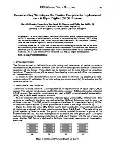
Deposition of SO42- can also be elevated in sites where S-rich fuels are consumed (e.g., emissions from ships and heavy freight), although S deposition is not a widespread problem in California (Bytnerowicz et al. 2016, Cox et al. 2013). Primary sources of N emissions in California are from fossil fuel burning, of which mobile sources are prominent, in addition to agricultural and industrial activities. Expressed on a per-N basis, emissions of N statewide are nearly evenly divided between reduced and oxidized forms, with NOx emissions only 9 percent higher than NH3 emissions. (Cox et al. 2013). In addition to agricultural emissions, NH3 emissions from light-duty vehicles equipped with three-way catalytic converters are also an important source (Bishop et al. 2010, Bishop and Stedman 2015). With recent downward trends in emissions of NOx in California (Bytnerowicz et al. 2016, Cox et al. 2013) and many other regions, reduced N forms (e.g., NH3 and NH4+) have become an increasingly large fraction of total N deposition (Du et al. 2014b). Regions of highest N deposition in California are near highly urbanized areas and areas affected by intensive agriculture. Urban air pollution is prominent in southern California and the central coast, while agricultural emissions are concentrated in the Central Valley. Urban and agricultural emissions in central and southern California result in elevated N deposition to wildlands in southern California and along the southern and western portions of the Sierra Nevada. Nitrogen deposition in California is lowest in the northern and eastern portions of the state (fig. 1.1). A characteristic feature of spatial patterns of N deposition in California are the steep declines in N deposition with distance from the source area. For example, in the San Bernardino National Forest in southern California, N deposition declines dramatically along a 45-km west-to-east gradient, from 71 kg ha-1 yr-1 near the town of Crestline to 8 kg ha-1 yr-1 near Barton Flats (Fenn et al. 2008). Such gradients are a function of high-deposition velocities of reactive N compounds such as HNO3 and

4

Nitrogen deposition kg N ha·1 yr1

- 30

deposition map data provided by R. F. Johnson, Center for Conservation Biology, UCR. Figure 1.1—Map of total annual nitrogen (N) deposition in California. Nitrogen deposition was calculated using the Community Multi-scale Air Quality Model for the most polluted two-thirds of the state on a 4-km resolution grid. The relatively unpolluted regions in northern and in the far southeastern corner of the state were simulated on a 36-km grid resolution (Fenn et al. 2010, Tonnesen et al. 2007). This was overlaid with vegetation cover data from the California Gap Analysis Project (Davis et al. 1998) to identify forested areas. Nitrogen deposition in mixed-conifer forest areas was adjusted based on the linear relationship with empirical throughfall data using the method previously described in Fenn et al. (2010).

5


NH3, and because of effective scavenging of N deposition in cloudwater by large tree canopies (Fenn and Poth 2004). However, long-range transport of N pollutants can occur as fine particulates and along river drainages such as the San Joaquin River drainage traversing the Sierra Nevada (Cisneros et al. 2010). The combined effects of O3 and N deposition contribute to increased aboveground growth, stand densification, and greater bark beetle activity and tree mortality in forests already stressed by periodic drought and long-term fire suppression.

1.4―Ecological and Environmental Effects of Nitrogen Deposition in California Ecological and environmental impacts of atmospheric N deposition reported in California (Fenn et al. 2003, 2008, 2010, 2011b, 2015b) include enhanced growth of invasive exotic grasses, local extirpation of N-sensitive epiphytic lichen species— leading to changes in lichen functional groups, increased bark beetle attacks and pine mortality in mixed-conifer forests, acidification of soils in forests and chaparral ecosystems, and N enrichment of remote lakes and changes in diatom assemblages. Additional impacts include elevated nitrate concentrations in streamwater and groundwater from chaparral and forested watersheds, increased greenhouse gas emissions, impaired visibility, and human health effects (Bytnerowicz et al. 2016). Recent studies indicate that N deposition can exacerbate fuel buildup in shrublands and desert ecosystems as a result of increased growth of invasive grasses. This increases the risk of fire and possible vegetation type change in these habitats (Fenn et al. 2010, 2015b). Similarly, the combined effects of O3 and N deposition contribute to increased aboveground growth, stand densification, and greater bark beetle activity and tree mortality in forests already stressed by periodic drought and long-term fire suppression. In summary, when chronic atmospheric N deposition, common in much of California, shifts ecosystems from a natural state of low N availability to a N-enriched condition, undesirable effects such as those listed above often ensue.

1.5―Monitoring Ozone and Nitrogenous Air Pollutants of Ecological Importance Air pollution monitoring can be done by way of “active monitoring.” As mentioned above, this involves the use of electronic equipment that is generally used to provide continuous measurements of pollutant concentrations in the atmosphere. In contrast, “passive monitoring” entails the deployment of samplers that do not require electrical power. Instead, passive samplers accumulate the pollutants of interest that diffuse onto a collection medium such as various types of filter disks, usually coated with a chemical chosen because of a selective affinity to the pollutant gas

6


USDA Forest Service

to be sampled. Such passive samplers, when exposed to the atmosphere for a given period, measure time-averaged atmospheric concentrations of key gaseous pollutants. The major reactive N gases (NO, NO2, HNO3, NH3) are routinely monitored with passive samplers (Bytnerowicz et al. 2005, Fenn et al. 2009). Passive samplers for measuring deposition fluxes capture ionic pollutants in solution from precipitation or throughfall as the ions are adsorbed onto IER material (Fenn and Poth 2004, Fenn et al. 2009). The primary advantage of passive samplers over methods of active monitoring is the potential to monitor at a much greater number of sites, including remote sites without electrical power or easy access (fig. 1.2). With sufficient sampling density—using passive samplers, maps or graphs can be generated from the monitoring data that show spatial distributions of air pollutant concentrations (Bytnerowicz et al. 2010, 2016, Frączek et al. 2003) or deposition across the monitoring network (figs. 1.3 and 1.4). Such widespread monitoring is not feasible with active collectors. With sufficient spatial sampling intensity, maps of throughfall deposition

Figure 1.2—Passive sampling approaches are particularly useful for monitoring remote sites, such as in the boreal forest in the Athabasca Oil Sands Region in northern Alberta, Canada, where many of the study sites are accessible only by helicopter.

7

USDA Forest Service


A

Passive monitoring 2005 • Monitoring sites - - Highways Lakes Urban

,----, L __ J National forest

c::J National park 40

80 Kilometers Witold Frączek, Environmental Systems Research Institute, Redlands, CA

20

0

B

•• • •

•

HNO,

2005, July 12- 27 Units: mlcrogramslm'

. . .

0.9-2.1 2.1-2.9 2.9 - 3.5 3.5 - 3.9 3.9 - 4.4 4.4-5.3 5.3 - 6.5 6.5 - 8.4

.

8.4 - 11 .1

•

11 .1 - 15.3 MofllDOl'fn,;IU4Jona

0

50

100

- - - -c::==Ki;;:_lom ;:::ae"le•r., !' - - -====

Figure 1.3—(A) Map of passive sampler network in southern California and (B) geographic information system mapping of average nitric acid (HNO3) concentrations across the sampler network for July 12–27, 2005.

8

50

ro :!:: Cl

40

~

Annual TF: S04-S

l.

.

~ .c:

95% cont

I

• •

Cl)

Year

Annual TF: NH4-N

o 20 , 0

T

•

a

c,i 15

e,

z

•

-

~ 10

2010 2011 2012 2013 2014

Regr

·•• • ••• 95% conf

z

······ • ·~·~ ···• •. :,,::::cF::~:i~,:::::, :::,::::.

20

40

60

80

100

120

I _!I ~ - • .'!

0

140

0

20

40

12

Year

•

10 .J

•

Annual TF: N03-N

o -.

--

a ~i

z,,

6

8 Z

4

~

•

2014

-

30

2008 2009 2010 2011 2012 2013

1:,.

•

60

80

100

120

•

2008

o

2009 2010 2011 2012 2013 2014 Regr

140

Distance (km)

Distance (km)

-

2008 2009

Annual TF : DIN

0

25 ~

T

"

-. 20 (tl

l--

.c

•

15

•

z

Regr

95% cont

Cl 10

•••·••• 95% cont

Year

5

2

To~ ~ ~ ~'-I

o-:---1 o

20

40

60 80 Distance (km)

100

120

140

o

I 0

20

40

60 80 Distance (km)

100

120

I 140

Figure 1.4—Annual throughfall (TF) deposition fluxes of SO4 -S, NH4 -N, and NO3-N (sulfate, ammonium, and nitrate, respectively) and dissolved inorganic nitrogen (DIN), with distance from the industrial center in the Athabasca Oil Sands Region in northern Alberta, Canada. Deposition was measured across the monitoring network from May 2008 to May 2014 with ion exchange resin TF deposition samplers. Values on the x-axis represent the distance (kilometers) of each monitoring site from the industrial center of the Athabasca Oil Sands Region, conf = confidence interval.

9


I 0

i

•

0

10

o

2009 2010 2011 2012 2013 2014 Regr

•

J 20

0

"

L>

~

-;;; 30

2008

T

•

25

Year

•

USDA Forest Service

60


across the landscape can be developed based on statistical models using relationships between landscape characteristics (e.g., topographic exposure, elevation, intensity of fog deposition, and vegetation type) and throughfall deposition fluxes (Fenn et al. 2009, Weathers et al. 2006). Monitoring throughfall, wet or bulk deposition, with conventional solution samplers requires that the samples be collected soon after a precipitation event to prevent microbial or other types of contamination (sometimes biocides are added to reduce this problem) or evaporation of the samples. Thus, frequent field sampling is needed. Consequently, a much greater number of samples are collected for laboratory analysis, although this is sometimes reduced by compositing samples from different precipitation events. In contrast, we generally use only two sampling periods per year for IER (passive) throughfall sampling. Another consideration is that if a large deposition network is needed to define deposition gradients or surfaces, collecting liquid samples on an event basis would require a number of field crews and greater logistical sampling complexity at unknown frequencies owing to the unpredictable timing of precipitation events. In addition, samples collected at remote sites are perishable and require storage at low temperatures during transit. In contrast, IER columns from passive deposition samplers are collected infrequently and are not time sensitive or perishable. We calculate that total annual deposition monitoring and analysis costs (for N and S) are six times higher with conventional throughfall samplers compared to a passive sampling approach in the first year when equipment must be purchased. In subsequent years, passive sampling is seven times less expensive. By comparison, active monitoring of O3 concentrations over the growing season using portable solar-powered monitors is approximately 2.5 times more expensive than monitoring with passive O3 samplers. Although the use of passive samplers is now common for monitoring gaseous pollutants, passive samplers have also been used in California to collect fogwater and rime ice. Ionic concentrations of atmospheric pollutants are highly concentrated in fogwater and rime ice compared to precipitation or snowfall (Berg et al. 1991, Fenn et al. 2000). Active collectors are also available for collecting cloudwater (Daube et al. 1987, Fenn et al. 2000, Roman et al. 2013). In some montane areas of California, N inputs from cloudwater or fog can constitute as much as one-third of the total annual N deposition (Fenn et al. 2000, Waldman et al. 1985). Note, however, that trees function as natural cloudwater collectors, resulting in elevated fluxes of N to the forest floor in throughfall (Fenn and Poth 2004). Rime ice formation results when supercooled cloud droplets freeze on impact with natural or human-made surfaces. We have deployed passive samplers for cloudwater (Fenn et

10


al. 2000) and rime ice (Berg et al. 1991) collection in California forests. Inasmuch as throughfall chemical flux measurements include estimates of the deposition of N and other pollutants to the canopy, including rime ice and cloudwater, we will not discuss rime ice or cloudwater samplers further in this report.

1.6―National Atmospheric Deposition Networks The largest atmospheric deposition network in the United States is the wet deposition monitoring program known as the National Atmospheric Deposition Program/ National Trends Nework (NADP/NTN) with 12 sites in California (http://nadp. sws.uiuc.edu/data/sites/NTN/?net=NTN). Only deposition in precipitation, including snowfall, is measured. The NADP network has provided much useful data on spatial and temporal deposition trends in the United States because it is the most spatially extensive and longest running network (since the late 1970s at some sites) in the United States (fig. 1.5). At a subset of the NADP sites, the atmospheric concentrations of some N and S pollutants are measured by the Clean Air Status and Trends Network (CASTNET) program, with five sites in California (http://epa.gov/ castnet/javaweb/index.html). From these data, dry deposition fluxes are determined from model simulations. However, dry deposition fluxes estimated by CASTNET are frequently much lower than empirical measurements from the same sites (Fenn et al. 2009, Sparks et al. 2008, Weathers et al. 2006). The NADP also operates the Ammonia Monitoring Network (AMoN) a network of passive samplers for measuring atmospheric concentrations of NH3. The AMoN was officially established in 2010 and currently consists of 67 sites, with three in California (http://nadp.sws.uiuc.edu/amon/). Commercially available Radiello diffusive tube passive samplers for NH3 are used at the monitoring sites. The intention is to continue expanding the network nationally. Empirical NH3 concentration data from AMoN are used in the hybrid Total Deposition Science Committee (TDEP) model that is based on simulations from the model Community Multi-scale Air Quality (CMAQ) (Byun and Schere 2006, Tonnesen et al. 2007) that is adjusted with empirical monitoring data where available (Schwede and Lear 2014). However, the NADP, CASTNET, and AMoN data are of limited use for ecosystem effects studies in California (Fenn et al. 2012). Because of the prominence of dry deposition in California, which NADP does not measure, the NADP wet deposition maps show California as one of the lowest pollution regions in the country (fig. 1.5), notwithstanding the fact that the highest N deposition in North America occurs in southern California. Likewise, cloud or fogwater deposition of N are important forms of N deposition inputs in coastal and montane regions of California that are influenced by atmospheric N emissions (Collett et al. 1990, Fenn

Because of the prominence of dry deposition in California, which NADP does not measure, the NADP wet deposition maps show California as one of the lowest pollution regions in the country, notwithstanding the fact that the highest N deposition in North America occurs in southern California.

11

8.0

6.0

2.0 0

Figure 1.5—Inorganic nitrogen (N) deposition (sum of nitrate [NO3-N] and ammonium [NH4 -N], in wet deposition in the continental United States in 2014 as reported by the National Atmospheric Deposition/National Trends Network.

National Atmospheric Deposition Program/National Trends Network, http:/nadp.isws.illinois.edu

~


12 (kg/ha)


et al. 2000, Fenn and Poth 2004, Templer et al. 2015), and the NADP wet deposition collectors do not effectively collect cloudwater. Furthermore, the sampling density for NADP (12 sites), and especially for AMoN (3 sites) and CASTNET (5 sites), are insufficient to describe N deposition in California. And, as mentioned above, CASTNET has been shown to underestimate dry deposition of N by a significant degree, including in California (Fenn et al. 2009, Sparks et al. 2008, Weathers et al. 2006).

1.7―Throughfall Deposition Monitoring Measuring throughfall deposition, the hydrologic flux of nutrients or pollutants washed from plant canopies during precipitation or snowmelt events, is a widely used method of estimating wet + dry deposition inputs of N or other compounds (Bleeker et al. 2003, Clarke et al. 2010, Draaijers et al. 1996, Hansen et al. 2013, Lovett and Lindberg 1993, Parker 1983, Thimonier 1998). The throughfall flux of nutrients from the canopy to the forest floor is an important part of ecosystem nutrient cycling. In polluted environments, the accumulation of dry-deposited compounds on canopy surfaces results in elevated nutrient fluxes to the forest floor. Many studies have related these increased throughfall fluxes of N or other pollutants to ecosystem effects. Although throughfall N deposition includes both wet and dry deposition of N, a fraction of atmospherically deposited N is retained by the canopy, and as a result, throughfall N deposition is generally lower than total N deposition, as has been shown in many regions (Clarke et al. 2010, Fenn and Bytnerowicz 1997, Hansen et al. 2013, Lovett and Lindberg 1993). Thus, at best, throughfall N deposition is a lower bound estimate of total N deposition. Because of canopy uptake of atmospheric N, in relatively low pollution sites N deposition measured under tree canopies (throughfall) is often lower than in canopy-free or open areas (referred to as bulk deposition). In contrast, throughfall deposition of S has often been reported to be a good surrogate for total S deposition (Clarke et al. 2010, Granat and Hällgren 1992, Hansen et al. 2013, Lindberg and Lovett 1992), but there are exceptions. Stemflow refers to the hydrologic flux of nutrients in solution running down tree trunks (Clarke et al. 2010, Parker 1983). Stemflow is much less frequently measured than throughfall because it generally represents a small proportion of the total deposition to the forest floor and requires additional equipment and effort. Stemflow can be measured by attaching spiral cords or collars around the base of tree trunks. Generally, less than 10 percent of the total deposition to the forest floor is from stemflow, but this differs by tree species. In beech or dense pine stands, for example, when precipitation intensity and duration are sufficient, stemflow 13


limitations of the throughfall technique, it is the most practical low-cost method for estimating deposition fluxes to forests and other ecosystems.

can constitute as much as 40 percent of the deposition (Draaijers et al. 1996). Ion exchange resin samplers have not been reported for measuring stemflow, but if the stemflow solutions were routed through IER columns, this could be accomplished. By definition, throughfall samples are only collected during precipitation events or as snow accumulated on tree canopies melts. This is problematic in arid climates such as mediterranean California where periods of little or no precipitation can span 3 to 6 months or longer (Fenn et al. 2000). Such long dry spells seem to result in greater underestimates of N deposition compared to throughfall measurements in more mesic climates or years with greater precipitation. This illustrates the need for including results from complementary approaches for estimating N deposition, especially during drought years. Notwithstanding the limitations of the throughfall technique, it is the most practical low-cost method for estimating deposition fluxes to forests and other ecosystems (fig. 1.6) (Clarke et al. 2010). This is why throughfall monitoring continues to be used in many studies, including large networks such as long-term regional, countrywide or continental-scale monitoring programs (Bleeker et al. 2003, Clarke et al. 2010, Fenn et al. 2008, Ferretti et al. 2014, Hansen et al. 2013).

USDA Forest Service

Notwithstanding the

measure throughfall? • Important process: the flux of nutrients from the canopy to the forest floor. • Integrates dry, wet, and occult deposition to the canopy. • Most practical approach for measuring atmospheric deposition at multiple sites. • Low tech: can be applied with minimal investment in equipment. son No; • Widely used: results can be compared on a worldwide database. Leaching

Nitrification

N In groundwater

Bedrock/parent material

Figure 1.6—Some of the key benefits of using throughfall deposition monitoring for estimating atmospheric deposition inputs to forests and other ecosystems. N = nitrogen, N2 = inert dinitrogen, N2O = nitrous oxide, NO = nitrogen oxide, NO3- = nitrate, and NH4+ = ammonium.

14


Chapter 2: Passive Monitoring for Atmospheric Concentrations of Gaseous Pollutants 2.1―Uses of Passive Samplers and Pollutants Commonly Measured The primary use of passive samplers is to measure time-averaged concentrations (typically 2- to 4-week averages) of gaseous pollutants, thus providing summary information on pollutant exposure at each monitoring site. Passive samplers for gaseous pollutants measure pollutant concentrations based on passive diffusion of the pollutant through barriers (filters, screens) or diffusion tubes, and onto the collection medium. The collection medium is chosen on the basis of its affinity to the pollutant gas to be sampled (Krupa and Legge 2000). In contrast, an “active sampler” involves the active movement of air through the air pollution monitor by a pump. Following field exposure of passive samplers, pollutant concentrations are determined by extraction of the sampler medium and measurement of the pollutant of interest. Atmospheric concentrations are determined from previously established linear relationships between concentrations of the pollutant as determined from reference methods using active samplers and passive sampler extraction data (Calatayud and Schaub 2013, Krupa and Legge 2000). Using passive samplers is a highly useful approach as it allows monitoring over much larger networks than is feasible with active samplers. Pollutants for which passive samplers have been commonly used in ecological-effects studies include nitrogen oxides (NOx), nitrogen dioxide (NO2), ammonia (NH3), nitric acid vapor (HNO3), sulfur dioxide (SO2), ozone (O3), and volatile organic compounds (VOCs) (see table 2.1). Concentrations of nitric oxide (NO) can be calculated as the difference between NOx and NO2. The key limitation of passive samplers is that the time-averaged data obtained do not describe diurnal patterns of pollutant exposure, which can be important when considering stomatal uptake and biological effects of pollutants (Krupa and Legge 2000). However, statistical procedures have been successfully used to estimate biologically relevant hourly O3 exposure indices from passive sampler O3 concentration data (Ferretti et al. 2012). Furthermore, portable solar-powered continuous O3 monitors are now available for real time O3 monitoring in remote locations (Burley et al. 2015). Data from passive samplers deployed with sufficient density can be used to develop pollutant exposure maps using geostatistical techniques (Fraczek et al. 2003), thus defining exposure to key pollutants across the landscape. Data on atmospheric concentrations of gaseous pollutants can be used to evaluate temporal trends in pollutant concentrations and to assess the potential for biological effects (Bytnerowicz et al. 2008, Cape et al. 2009). Concentration data for nitrogenous 15


Table 2.1―Characteristics of passive samplers for ozone and nitrogen and sulfur pollutants, including common analytical methods

Pollutant HNO3 + HNO2 NO2 b

NOx NO NH3 O3 SO2

Collection mediuma Nylasorb (nylon filters) Filters coated with triethanolamine (TEA) TEA + an oxidizing agent Calculated as the difference between NOx and NO2 Filters coated with citric acid Pads coated with sodium nitrite Filters coated with TEA

Ion measured in extract -

Analytical methoda

NO3 NO2-

Ion chromatography Colorimetrically

NO2-

Colorimetrically

c

NH4+ NO3SO42-

Colorimetrically Ion chromatography Ion chromatography

Literature references Bytnerowicz et al. 2005 Ogawa & Co., USA 2006 As above As above Roadman et al. 2003 Koutrakis et al. 1993 Ogawa & Co., USA 2006

HNO3 = nitric acid,, HNO2 = nitrous acid, NO3- = nitrate, NO2 = nitrogen dioxide, NH3 = ammonia, NO = nitric oxide, O3 = ozone, NH4+ = ammonium, SO2 = sulfur dioxide, SO42- = sulfate. a The analytical approaches and the collection media listed in the table are the ones used in our laboratory, but the ions mentioned in the table can all be analyzed with either colorimetric or chromatographic techniques. b

NOx refers to the sum of concentrations of NO and NO2.

c

When atmospheric NH3 reacts with the citric acid, it forms diammonium citrate [(NH4)2C6H6O7], which is extracted from the filters and concentrations of NH4+ determined colorimetrically.

pollutants can also be used to calculate dry deposition fluxes to the ecosystem, an approach commonly known as the inferential method, which is summarized in section 4.3 (Bytnerowicz et al. 2015). Passive samplers used to monitor HNO3 have also been used for stable nitrogen (N) isotope analysis of the collected HNO3 (Bell et al. 2014, Elliott et al. 2009).

2.2―Design of Passive Samplers Although there are various designs for passive samplers (Krupa and Legge 2000), we will focus on two types of passive samplers that we have commonly been used in field campaigns in California. The first is a widely used passive sampler generally referred to as the Ogawa sampler (fig. 2.1) (Koutrakis et al. 1993, Fenn et al. 2009, Roadman et al. 2003). This sampler is used to measure NH3, NO2, NOx, SO2, and O3. The sampler is made of Teflon® with a Teflon end cap with precisiondrilled holes followed by a stainless steel mesh serving as the diffusion barrier. The sampler also requires the use of a shelter to protect the sampler from precipitation (fig. 2.1). The respective pollutant to be sampled is collected on cellulose filters (two per sampler) coated with reagents known to react to the pollutant of interest (Fenn et al. 2009, Roadman et al. 2003). Generally, one sampler per pollutant type (e.g., NH3, NO2) is installed per site, yielding two replicate samples. 16

USDA Forest Service


B

USDA Forest Service

A

Figure 2.1—(A) An assembly of passive samplers for measuring average concentrations of gaseous pollutants in the atmosphere over the time of exposure. Ogawa samplers for measuring ozone (O3), ammonia (NH3), nitrogen dioxide (NO2), and nitrogen oxides (NOx) are shown along with three replicate nitric acid (HNO3) vapor samplers. Typical units of measure for gaseous pollutant concentrations in the atmosphere are micrograms per cubic meter (µg m-3; e.g., µg NH3 m-3 or µg NH3-N m-3). (B) Closeup view of an Ogawa passive sampler.

17


The second sampler we have widely deployed in field studies is a passive sampler for measuring HNO3 + nitrous acid (HNO2) concentrations (fig. 2-1). This nitric acid sampler is based on quantitative absorption of these gases to nylon filters (Bytnerowicz et al. 2001, 2005). The sampler uses a Teflon membrane for controlling airflow to the nylon filter (Bytnerowicz et al. 2005). Generally, three HNO3 samplers are deployed at each site, yielding three replicate samples. Although HNO3 is generally the primary pollutant of interest when deploying these samplers, as mentioned, both HNO3 and HNO2 are absorbed by the nylon filters. Ecologically, both of these gases can be important sources of atmospheric N, and, in this sense, the total of these two gases is important to measure. The ratio of HNO2/ HNO3 in the atmosphere varies in time and space depending on ambient photochemical processes (Finlayson-Pitts and Pitts 1986) but cannot be determined by this sampler. Collection media coated or impregnated with sodium chloride (NaCl) can be used to quantitatively capture HNO3 from air without also collecting HNO2 (Allegrini and De Santis 1989, Allegrini et al. 1987). In preliminary trials at our lab, we coated cellulose, glass and quartz filters with 0.25 N NaCl and used these in the HNO3 + HNO2 sampler (Bytnerowicz et al. 2005) to measure atmospheric concentrations of HNO3 only. Results were in agreement with HNO3 concentrations as measured by a colocated annular denuder active sampling system (Koutrakis et al. 1988; Bytnerowicz, unpublished data). These results demonstrate conceptually that samplers with filters coated with NaCl may be useful in measuring only HNO3, while colocated samplers with nylon filter could be used to measure exposure to HNO3 + HNO2. Average concentrations of HNO2 during the exposure period could be determined by difference between the results of the two filter types. However, further field tests would be needed to further validate this approach.

2.3―Preparation and Assembly of Passive Samplers Key in preparing passive samplers for field deployment is to handle them carefully to avoid contamination during assembly, transport to and from the field (Puchalski et al. 2011), storage, disassembly, and extraction of filter pads. Samplers should be prepared in a clean room or space, preferably in a clean air hood. Precautions include the use of gloves to avoid touching the samplers with bare hands, handling filters with forceps, covering tables or work benches with clean laboratory paper, and storing samplers in clean containers and storage bags to avoid atmospheric exposure prior to deployment. Unexposed blank or control filters stored in sealed containers are kept in the lab and later analyzed along with the field-exposed sampler filters; the ionic content from extracts of these filters are used to blank-correct 18


the samplers exposed in the field. More detailed procedures for preparation and assembly of passive samplers are given in appendix 1.

2.4―Calibration of Passive Samplers To derive atmospheric concentrations from the ionic content of the passive sampler filter extracts, a calibration curve relating the extract data with atmospheric exposures must be used. Such calibration curves are developed by measuring atmospheric concentrations with a reference method (active sampler) and collocated passive samplers (fig. 2.2). Then results from each of the two methods are plotted and tested for linearity in the relationship (fig. 2.3). Passive samplers should only be used in environments in which calibration curves have been established. Environmental conditions such as high winds, temperature, dust or other pollutants, or high humidity can potentially affect the performance of passive samplers (Bytnerowicz et al. 2005, Koutrakis et al. 1993, Krupa and Legge 2000). For these reasons, calibrations against reference methods are ideally obtained under field conditions in the areas of interest during the seasons of the year to be monitored. However, in practice, such calibrations are often not practical and must be done at least in locations with similar climatic conditions.

The primary use of passive samplers is to measure time-averaged concentrations (typically 2- to 4-week averages) of gaseous pollutants, thus providing summary information on pollutant exposure at each monitoring site.

2.5―Field Deployment of Passive Samplers In selecting monitoring sites it is preferable to avoid steep slopes, and find sites located on plateaus if possible. In the Sierra Nevada of California, sites with a western aspect are preferred because the majority of the air pollution load originates in the California Central Valley to the west. If colocated with vegetation-effects study plots, the passive sampler location should be at the same elevation. When installing passive samplers in tall vegetation, such as forests or woodlands, choose a monitoring location that has an open fetch or corridor for air mass transport from the expected pollution source area so that pollution exposure in the broader study area is effectively characterized. At sites within or near a forest stand, locate passive monitors in an opening at a distance from the stand of at least two to three times the height of the tallest trees (fig. 2.4). Often it is difficult to find large stand openings across a monitoring network. Scarcely dispersed trees or shrubs, not directly obstructing airflow to the samplers should not be problematic. Exceptions to this rule could include studies in which the effects of canopy or stand position on pollution exposure also are being studied. Passive samplers should typically be placed about 2 m above ground level. At this height, pollutant concentrations represent ambient concentrations that are relatively unaffected by deposition to soil surfaces or short vegetation. At such a 19

A

USDA Forest Service

USDA Forest Service,


B

Figure 2.2—(A) Honeycomb denuder/filter pack system (active sampler unit strapped to the vertical post) used for calibration of ammonia and nitric acid passive samplers (mounted on the upper cross bars); and (B) a passive sampler calibration experiment at the Pacific Southwest Research Station Riverside Laboratory. Note that electricity is only required for the active samplers in the calibration, not the passive samplers.

A

Extractable NH.' vs. NH 3 dose 8000

1400

7000

1200

6000

}: ~

~

R'= 0.99S5

5000

E

j

E

~ 4000

., ..,"'0 3000

i

y = 93.079x R' = 0.9613

}:: 1000

y = 858.79x

B

Extractab le N03 - vs. HNO 3 dose

600

i

400

0

2000

800

,,:

200

1000 0 0 .0

2.0

6,0 4.0 119 NH,• per filter

8.0

10.0

0 0

2

4

6

8 10 1•9 No.- per filter

12

14

16

Figure 2.3—(A) Calibration curve for calculating average atmospheric concentrations of ammonia (NH3) from passive samplers exposed in the field. To obtain NH3 concentrations in micrograms per cubic meter (µg m-3), the NH3 dose on the Y-axis (from the active sampler) is divided by hours of exposure. The linear regression shows the correlation between concentrations of ammonium (NH4+) in the passive sampler filter extracts and atmospheric concentration of NH3 as measured with an active sampler. (B) Calibration curve for calculating average atmospheric nitric acid vapor (HNO3) concentrations from passive samplers exposed in the field. (Left figure for NH3 dose courtesy of USDA Forest Service, Pacific Southwest Research Station. Figure on the right for HNO3 dose reprinted from Bytnerowicz et al. (2005) with permission from Elsevier).

20

Andrzej Bytnerowicz, USDA Forest Service


Figure 2.4—Multiple passive samplers installed at a single field site in the White Mountains of California. Samplers are placed away from trees.

height, it is also easy for operators to install and change the samplers (fig. 2.5). It is recommended that two to three replicate passive sampler media (i.e., filter disks) be deployed at each monitoring location. Frequently passive samplers for measuring several pollutants of interest are deployed simultaneously, depending on the aims of the study (fig. 2.6). Passive samplers also can be placed on towers above the vegetative canopy (fig. 2.7), which allows for sampling of incoming air pollution to the site. Because vegetation takes up gaseous pollutants, passive samplers should be at least 1.5 m above the canopy to avoid canopy effects on atmospheric concentrations. However, samplers should be no more than 3 m above the canopy to ensure that exposure data are relevant to vegetative exposures in the sampling region. The most common exposure period for passive samplers is 2 weeks, although both shorter or longer periods can be sampled. In remote locations and where pollutant levels are low, exposure periods of 1 or 2 months have also been used (Hsu et al. 2016). With longer exposures, the resulting average pollutant concentration covers a longer period, with less time resolution. For some applications, this makes the data less useful because little is known about pollutant concentration dynamics over an extended period. Passive samplers should be transported to and from field sites in clean, sealed air-tight containers and plastic bags to prevent contamination in transit. Containers 21




Figure 2.5—A change-out of passive samplers at Devils Postpile National Monument California (the Granite Dome site).

Figure 2.6—Closeup view of a setup for passive monitoring of multiple gaseous pollutants. The yellow housing unit contains passive samplers for volatile organic compounds (Burley et al. 2015), illustrating an additional type of pollutant that can be passively sampled.

22



Figure 2.7—A suite of passive samplers placed on a tower above the forest canopy in the Athabasca Oil Sands Region in northern Alberta, Canada, illustrating that the deployment of samplers can be in a variety of physical configurations. The passive samplers are deployed and accessed for change-out by a cable-and-pulley system.

and procedures used to transport samplers and travel blanks to and from field sites should be carefully monitored for possible contamination. Travel blanks should be incorporated into monitoring plans to account for background levels and blank correction and to detect potential contamination problems during transit. For example, Puchalski et al. (2011) discovered that the plastic vials used to transport passive samplers for NH3 were emitting NH3 during warm weather. It was found that transporting the NH3 samplers in all glass vials with Teflon-lined lids solved this problem. Such contamination problems can occur with passive samplers for other pollutants as well. As another illustration of the use of inappropriate materials, we have found that Teflon tape from hardware stores is unsuitable for sealing travel containers in passive monitoring studies because of contamination issues. Use clean disposable gloves when placing the samplers on the mounting pole or stand and when collecting the sampler following the field exposure period (fig. 2.5). However, even “clean” disposable gloves can be a source of contamination, illustrating that

23


During all phases of preparing, deploying, and processing the passive samplers, use extreme care to prevent contamination.

all potential surfaces and supplies used should be evaluated as potential contamination sources. During all phases of preparing, deploying, and processing the passive samplers, use extreme care to prevent contamination. See appendix 1 for a sample protocol for field deployment of passive samplers.

2.6―Laboratory Methods of Analysis Following Field Exposure It is beyond the scope of this report to discuss chemical analysis methods in detail, particularly because details of such methods can be obtained from manufacturers of analytical equipment and elsewhere and because methods differ considerably among laboratories depending on the design, make, and model of instrumentation used. The Ogawa and HNO3 samplers discussed herein require extraction of the

Results from air pollution monitoring networks can be converted into maps of air pollution distribution that are useful for scientists, air resource and land managers, and decisionmakers.

24

collection medium and subsequent analysis of the pollutant of interest in the filter extracts. Table 2.1 lists the type of collection medium used, the ion measured in each extract solution, and suggested analytical techniques for passive samplers of O3, and each of the N pollutants considered here. For each of these passive samplers, the collection medium (filter) is extracted with deionized/distilled water. On occasion, we have found that when monitoring at relatively unpolluted sites, particularly during seasons when pollutant concentrations are at their lowest, the ionic content of the filter extracts can be below the analytical detection limit. Such low pollution levels are below the thresholds expected to cause ecological harm. In these situations, exposure periods greater than 2 weeks may be more appropriate.

2.7―Data Processing, Calculation of Atmospheric Concentrations, and Pollutant Mapping Raw data from chemical analysis of sampler extractions will provide ionic concentration data of the extract solutions, which based on extract volumes must then be converted to total ionic content extracted from the sampler. Using the example of the HNO3 samplers, the µg NO3-/filter can be converted to atmospheric concentrations of HNO3 + HNO2 based on the previously established calibration curve (Bytnerowicz et al. 2005). Example calculations for O3, NOx, NO2, NO, HNO3, and NH3 are shown in appendix 1. Results from air pollution monitoring networks can be converted into maps of air pollution distribution (fig. 1.3) that are useful for scientists, air resource and land managers, and decisionmakers using geostatistics (Frączek et al. 2003). In our applications, we have used various versions of the Geostatistical Analyst software, which is an extension of ArcGIS software developed by the Environmental Systems Research Institute (ESRI, Redlands, California). Geostatistical Analyst uses values


measured at monitoring network sites and interpolates them into a continuous surface of pollutant distribution using various techniques such as kriging, cokriging, or inverse distance weighing (Johnston et al. 2003). In addition to surfaces representing spatial changes in pollutant concentrations, uncertainty of predictions, called the prediction standard error, can also be calculated when the network density allows for using simple kriging (Bytnerowicz et al. 2010). Physiological measurements of foliar stomatal uptake of O3 is the most appropriate metric for evaluating plant responses to O3. However, because of the lack of stomatal conductance data for most of the tree species, simple O3 exposure indices calculated from hourly ambient O3 concentrations are more often used to evaluate potential responses of plants to O3 exposure (Musselman and Korfmacher 2014). Average O3 concentrations (e.g., 2-week averages) obtained from passive O3 samplers can be used to estimate hourly O3 concentrations at passive sampler monitoring sites using statistical models that couple O3 concentration data from passive samplers with meteorological variables (Cisneros et al. 2010, Krupa et al. 2003). Alternatively, portable, solar-powered active ozone monitors can be deployed in select locations (Burley et al. 2015).

25


26


Chapter 3: Deposition Monitoring With Ion Exchange Resin (IER) Collectors 3.1―Uses of IER Collectors and Definition of Terms Ion exchange resin (IER) samplers are used to measure deposition in precipitation and throughfall. Because these samplers use funnels constantly exposed to the atmosphere to capture the precipitation or throughfall solutions, such measurements are referred to as bulk deposition measurements. The term “bulk” refers to the fact that some level of dry deposition accumulates on the funnel sampler during dry periods and becomes part of the deposition measurement. This is in contrast to wet-only samplers that are closed by a lid during dry periods and only open during precipitation events (Fenn et al. 2009, Glaubig and Gomez 1994). In the atmospheric deposition literature, the term ”bulk deposition” has long been used specifically in reference to precipitation samples collected in open canopy-free areas with continuously exposed collectors. These are more commonly funnel- or cylindrical-shaped collectors, but trough collectors have also been used (Bleeker et al. 2003). However, with few exceptions (Fenn and Bytnerowicz 1997, Glaubig and Gomez 1994), throughfall samplers are continuously exposed to the atmosphere and thus collect dry deposition on the collector surfaces during dry periods. As such, these throughfall measurements are bulk throughfall collections, but usually are simply referred to as throughfall or throughfall deposition. However, such continuously exposed funnel, bucket, or trough collectors are not efficient dry deposition samplers, and the amount of dry deposition deposited directly to the collector from the atmosphere is considered minor compared to the interactions of dry deposition with plant and tree canopies and their much larger and reactive surface areas for dry deposition collection (Du et al. 2014a). Sometimes there has been a perception that throughfall deposition fluxes measured with IER throughfall collectors is a different flux measurement than fluxes measured with conventional throughfall solution samplers. In actuality, the throughfall input measurements are equivalent for both methods as has been demonstrated in field trials (Fenn and Poth 2004, Fenn et al. 2002). The ultimate -1 -1 flux measurements (i.e., kilograms per hectare per year [kg N ha yr ]) are identical. The principal difference between the two approaches is that with IER samplers, no liquid samples are collected in the field. Instead, ions in throughfall solutions are adsorbed and accumulated by the IER columns as the liquid percolates through the column by gravity flow. Typically, IER columns are left in the field for about 6 months, accumulating ions from solution with each precipitation or snowmelt event. At the end of the sampling period, the IER columns are brought back to the laboratory for extraction of the adsorbed ions and chemical analysis of ions in the extractant solution. In contrast, with conventional throughfall samplers, solutions 27


are collected repeatedly, either on an event or periodic basis. Total volumes of the collected solutions are measured and samples analysed for ionic concentrations. In the end, with both methods, the amount of ionic deposition to the throughfall collector is determined, ultimately resulting in data expressed as deposition of a given ion or element per land area over time (i.e., kg NO3-N ha-1 yr-1).

3.2―Pollutants Measured With IER Collectors The most widespread use of IER collectors has been to measure deposition of nitrate (NO3-), ammonium (NH4+), and sulfate (SO42-). Deposition of chloride (Cl-), phosphate (PO42-), and cations such as calcium (Ca2+), magnesium (Mg2+), sodium (Na+), and potassium (K+) can also be measured (Fenn et al. 2015a, Simkin et al. 2004). Typical extractants used to remove the ions of interest from IER columns prior to analysis and associated methods of ionic analysis are listed in table 3.1. The sum of NO3-N and NH4-N in solution is commonly referred to as dissolved inorganic nitrogen or DIN, and this is what is typically measured in throughfall or bulk deposition. Dissolved organic nitrogen (DON) deposition fluxes are also a significant portion of the atmospheric input flux in many cases (Cornell 2011), although DON is much less frequently measured, largely because the analysis is less straightforward and because of the uncertain composition and sources of the mixture of organic N compounds. Dissolved organic nitrogen can be measured in the throughfall solutions collected in conventional samplers, but techniques have not been developed for quantitative extraction of DON from IER columns. Dissolved organic nitrogen is actually composed of many organic compounds that contain N, so this is a complex mixture of compounds and would likely require a different type of exchange resin than for inorganic N. The feasibility of measuring DON with a variety of IER types would need to be tested. Likewise, the pH or hydrogen ion (H+) concentration of precipitation or throughfall solutions can be measured after sampling with conventional samplers. However, the acidity of precipitation or throughfall, and the concentrations in solution of any ions deposited, cannot be determined with IER samplers because throughfall or precipitation solutions per se are not collected. Instead, anions and cations are generally extracted from the IER columns with a strong salt solution, which precludes the possibility of measuring the pH or ionic concentration of the original solution. In several studies, the natural abundance isotopic signatures of NO3- (Clow et al. 2015, Nanus et al. 2008, Proemse et al. 2013, Templer and Weathers 2011) and SO42- (Proemse et al. 2012) in IER extracts have been determined. Isotopic signatures of atmospheric deposition such as that determined with IER samples can help identify the emissions sources from which the N or sulfur (S) pollutants originated. 28


Table 3.1―Ions commonly measured with ion exchange resin (IER) deposition samplersa

Ion

Typical extractant

Analytical methodb

Literature references

NO3-

1N KI or 2N KCl

Ion chromatography or colorimetrically

NO3NH4+

1N NaCl 1N KI or 2N KCl

SO42PO42ClNa+, Mg2+, Ca2+

1N KI 1N KI 1N KI 2N KClc

+ + 2+ 2+ K , Na , Mg , Ca

1N ammonium acetate (NH4C2H3O2); or 0.5N or 1N HCld 2N H2SO4

Colorimetrically Ion chromatography or colorimetrically Ion chromatography Ion chromatography Ion chromatography ICP-AES (inductively coupled plasma-atomic emission spectroscopy) ICP-AES

Fenn and Poth 2004; Fenn et al. 2013, 2015a; Simkin et al. 2004 Köhler et al. (2012) Fenn and Poth 2004; Fenn et al. 2013, 2015a Fenn et al. 2013, 2015a Fenn et al. 2013, 2015a Simkin et al. 2004 Fenn et al. 2015a

K+, Na+, Mg2+, Ca2+, Al, Fe, Mn, PO42-

ICP-OES

Fenn, unpublished data; Yamashita et al. (2014) describe the HCl extraction. Köhler et al. (2012)

NO3- = nitrate, NH4+ = ammonium, SO42- = sulfate, PO42- = phosphate, Cl- = chloride, Na+ = sodium, Mg2+ = magnesium, Ca2+= calcium, K+ = potassium, Al = aluminum, Fe = iron, Mn = manganese. a

Negatively charged ions are captured from solution by anion exchange resin beads and positively charged ions by cation exchange resin beads. Mixed-bed resin (containing a mixture of cation and anion exchange resin beads) can be used to capture both cations and anions. b

Analytical methods other than those listed can be used. Methods listed in the table are those described in the literature references given. c

Note that in Fenn et al. (2015a), the IER columns were actually first extracted with 1N KI for analyzing the extracts for + 22concentrations of NO3 , NH4 , SO4 , and PO4 . Then the same IER columns were further extracted with 2N KCl to extract the remaining base cations. d

Ammonium acetate is a stronger extractant than HCl, particularly for extraction of Ca2+ from the IER columns, although either extractant can be used. We use ammonium acetate routinely in our laboratory for extracting base cations. Other extractants such as BaCl2 should also work for extracting base cations, but barium is more toxic than the extractants listed.

3.3―Design and Construction of IER Collectors Ion exchange resin throughfall or precipitation collectors are based on the same design as more conventional samplers except that in lieu of a bottle for collecting the solution from the funnel (or whatever type of recipient is deployed), an IER column is attached to the funnel to capture ions from the solution as it drains through the column (fig. 3.1). The deionized liquid is then allowed to drain onto the ground and is not saved for analysis. This is the key difference between IER collectors and conventional samplers (figs. 3.2 and 3.3). The core components of an IER throughfall sampler consist of a funnel (fig. 3.4) or cylindrical solution collecting device that is connected to a column filled 29

USDA Forest Service


Exchange Resin (IER) Throughfall Collector

Funnel

Ions in throughfall or precipitation samples are adsorbed by anion and cation exchange resin beads within the IER column. . After exposure, ions of interest are extracted from the columns, analyzed and deposition fluxes calculated.

Fence post

Figure 3.1—Photograph of an IER bulk deposition collector. Ion exchange resin collectors are used to collect precipitation (placed in open, canopy-free areas) or throughfall (placed under tree or other vegetation canopies) deposition samples.

30

Hėctor García-Gomez, Center for Ecotoxicology of Air Pollution, Madrid, Spain


Figure 3.2—Ion exchange resin (IER) throughfall collector on the left and conventional throughfall solution collector on the right—in a holm oak stand near Madrid Spain (García-Gómez et al. 2016). Both collectors are covered by a white tube designed to block direct solar radiation. For the collector on the left, the narrower shade tube covers the IER column. For the collector on the right, the shade tube is larger in diameter to accommodate a bottle connected to the funnel that collects the throughfall solution. Both collector types use the same funnel and bird rings. In this particular site, no snow tubes are needed.

31

Hėctor García-Gomez, Center for Ecotoxicology of Air Pollution, Madrid, Spain


USDA Forest Service

Figure 3.3—Ion exchange resin (IER) throughfall collector. Photograph is similar to figure 3.2 except that the shade tube covering the ion exchange resin (IER) column has been lowered to reveal the IER column. Also note the opaque cover over the liquid solution collector on the right to protect the sample from sunlight and reduce warming of the sampler.

Figure 3.4—Inside view of a funnel used for monitoring throughfall or bulk deposition with ion exchange resin (IER) collectors. The disk in the center of the funnel is to keep coarse litter out of the IER columns. Polyester floss is also inserted on the top of the IER column as a fine filter.

32


with IER beads. The bottom end of the IER column includes a cap with a threaded drainage hole or slit cut in the cap. A shade tube is sometimes used to cover the IER column and prevent direct solar radiation to the column (figs. 3.2 and 3.3). There are many permutations upon this design, including varying diameters and heights of funnels and different lengths of IER columns. For collecting throughfall under lower lying vegetation, such as chaparral or other shrubs, the IER collector design is modified to fit under low-lying shrubs. For example, we use IER columns of 5 to 6 cm in length and shorter funnels so that the collector can easily be placed under low-lying shrub canopies (fig. 3.5). Particularly for samplers placed in open or canopy-free areas, it is recommended to use some type of protection against bird droppings by attaching a bird sitting ring (fig. 3.6) or bird rejection device above the funnel or snow tube to reduce the occurrence of sample contamination by bird droppings (see section 3.6). The IER collectors used in field monitoring studies can be constructed of simple components readily available at hardware or irrigation supply companies. Funnels of various sizes and designs can be obtained from auto, hardware, scientific, or general suppliers accessible via the Internet. The main requirement is that the funnels are made of inert materials that are not contaminated with the ions of interest and that the sample solution be efficiently collected and routed to the IER column so that the ions are adsorbed by the IER beads as the solution percolates through the column. Components of the IER collectors that come in contact with the sample solutions in the field should be tested in leaching studies in the laboratory to be sure they are not a source of the ions to be monitored in deposition. Nylon material should be avoided because of its known affinity for nitric acid vapor (HNO3) (see section 2.2), which could confound the results when monitoring for NO3-N deposition. Here we give an example of a potentially problematic collector design (Klopatek et al. (2006) placed in short cylindrical (i.e., 5-cm) IER collectors along a vertical profile within tree canopies to measure throughfall deposition at different heights within the canopy. This study took place in south-central Washington state. When we used these same collectors for sampling throughfall under coastal sage scrub vegetation in the Los Angeles Air Basin, we found evidence of high levels of background contamination of NH4+, NO3-, and SO42- in the field blanks exposed only to the dry atmosphere for 7 months. In this collector design (Klopatek et al. 2006), the exchange resin is sandwiched between two pieces of fine mesh nylon netting and otherwise directly exposed to the atmosphere in the cylinder. Tests in Riverside, California, showed that IER directly exposed to the atmosphere during the summer smog season in petri dishes, or placed in the cylindrical samplers in

The IER collectors used in field monitoring studies can be constructed of simple components readily available at hardware or irrigation supply companies.

The main requirement is that the funnels are made of inert materials that are not contaminated with the ions of interest and that the sample solution be efficiently collected and routed to the IER column.

33

USDA Forest Service


A

B

Figure 3.5—Two different designs of ion exchange resin throughfall collectors for monitoring nitrogen deposition under low-lying chaparral vegetation. The funnel in photo B (24 cm diameter) is larger than the funnel in photo A (11 cm diameter). The larger diameter is considered a more effective throughfall sampling size. Notice the yellow and orange colored nitrophilous lichen species (Xanthomendoza spp.) colonizing the woody chaparral branches in photo A.

34

USDA Forest Service


Figure 3.6—An ion exchange resin bulk deposition sampler mounted on the fence of an air pollution monitoring station. A snow tube to allow for snow collection and accumulation and a bird sitting ring to prevent contamination of the sample by bird droppings are attached to the collector.

a fume hood with a steady airflow resulted in high levels of N in the IER extract solutions. We concluded that IER samplers with the IER directly exposed to pollutants and moisture in the atmosphere is an inappropriate design. Apparently, under these conditions, the IER can adsorb reactive N from the atmosphere and much of the background SO42- may result from breakdown of the exposed resin, because background levels of SO42- were greater than for NH4+ or NO3-. Furthermore, the use of nylon mesh to contain the IER is also not advised because of the high affinity of nylon for HNO2 and HNO3 (Bytnerowicz et al. 2005, section 2.2, table 2.1). Thus, adsorption of HNO2 and HNO3 by the nylon mesh may explain why background levels for NO3-, although elevated, were less than for NH4+ in the IER extracts, especially in the more polluted sites. Based on previous throughfall studies in forest ecosystems, it has been recommended that funnel openings be at least 20 cm in diameter and funnels with vertical sidewalls and beveled top edges are also preferred (Bleeker et al. 2003, Clarke et al. 2010). Once the collector components are assembled, they should be washed, rinsed 35


with distilled water, and dried. Place collectors in clean bags to keep them clean during storage and transport to the field. Do not touch the inner surfaces of the funnels or other parts of the collector with hands or anything that could contaminate the collectors. Different types and commercial varieties of IER beads can be used within the IER columns. Ion exchange resin beads are marketed by scientific suppliers, but the prices from such suppliers tend to be cost prohibitive if many samplers are to be deployed. We purchase analytical grade IER beads in bulk from a water purification company. Because both NO3- (an anion) and NH4+ (a cation) deposition are important to measure in N-deposition studies, mixed-bed IER, containing anion and cation exchange resin beads, are commonly used in IER collectors (Fenn and Poth 2004, Kjønaas 1999b). Furthermore, it is often useful to monitor deposition of N and S, and possibly base cations in the same study (Fenn et al. 2015a, Watmough et al. 2014). Alternatively, anion exchange resins can be used if only anions such as NO3- and Cl- are being measured (Simkin et al. 2004). If only base cations are being measured, one could use only cation exchange resin beads in the IER columns. Although any of various collector designs can be employed for collecting throughfall or bulk deposition, for our recent forest monitoring studies, the collector details are as follows: the IER columns (6 to 8 in [15.24 to 20.32 cm] in length) are filled with Amberlite™ IRN 150 mixed-bed analytical grade ion exchange resin beads prerinsed with distilled deionized water. Precipitation or throughfall samples are collected by a polyethylene funnel or snow tube and channeled through the resin column, where ions are retained by the IER. The inner diameter of the funnels used for the IER collectors is 21.1 cm, and the funnel collectors have a vertical wall 10 cm in height. For winter collection in sites with significant snowfall, snow tubes with an inner diameter of 20.2 cm are inserted into the funnels to capture snow (see section 3.5 and fig. 3.7).

3.4―Field Deployment of IER Collectors: Placement, Number of Replicates, and Open vs. Throughfall Collectors Field deployment of IER collectors is done the same as for conventional samplers. Details regarding the number of samplers to install, their placement in the field, exposure times or change-out frequency for the IER columns are largely dependent on the objectives of the study, statistical requirements, and available resources. Reviews of throughfall sampling methods have already been published (Bleeker et al. 2003, Clarke et al. 2010, Draaijers et al. 1996, Hansen et al. 2013, Thimonier 1998).

36

USDA Forest Service


Two types of deposition monitoring are used to measure inputs with IER collectors—bulk deposition in open areas and throughfall sampling with collectors placed under tree canopies.

Figure 3.7—An ion exchange resin (IER) sampler with snow tube attached. Notice that the IER column is not yet attached to the bottom of the sampler. A new IER column is attached at the beginning of each new exposure period, typically for 5- to 6-month intervals.

Two types of deposition monitoring are used to measure inputs with IER collectors—bulk deposition in open areas (referred to simply as bulk deposition; figs. 3.8 and 3.9) and throughfall sampling with collectors placed under tree canopies (fig. 3.10). Bulk deposition is composed primarily of wet deposition with an unknown background level of dry deposition but can be considered as an approximation of 37



USDA Forest Service

Figure 3.8—Installation of ion exchange resin bulk deposition samplers in a forest clearing in the Lake Tahoe basin. Passive samplers for gaseous pollutants and a battery/solar-powered active ozone monitor (Burley et al. 2015) were also installed at this study site.

Figure 3.9—Bulk deposition ion exchange resin (IER) samplers being installed in a bog, a natural forest clearing, in a remote boreal forest site in northern Alberta, Canada. Notice the bird rings installed on the funnel collectors to discourage birds from perching on the funnels. The white tubes function as a shade covering over the IER columns, to prevent direct sun exposure of the IER columns.

38

USDA Forest Service


Figure 3.10—Ion exchange resin throughfall collectors, (left) with and (right) without snow tube attached.

wet deposition in most cases. Throughfall deposition in essence uses tree or other vegetation canopy as a collecting surface for dry-deposited pollutants and for fog or cloudwater-deposited pollutants (fig. 3.11). As such, throughfall deposition fluxes include estimates of wet, dry, and cloudwater deposition of N. However, throughfall generally underestimates total N deposition because of canopy retention of N (Lovett and Lindberg 1993). Bulk deposition collectors intended for bulk deposition need to be placed in stand openings large enough to avoid blowoff from adjacent canopies such as during windy storm events. The number of throughfall collectors needed for a particular degree of precision is specific to a given forest site and the ions to be measured. However, fewer collectors are needed for measuring deposition fluxes than for chemical concentration (i.e., when collecting liquid samples with conventional throughfall collectors). This is because ionic concentration data can differ widely between samples or sampling dates, while in comparison, ionic fluxes are moderated by the interaction between throughfall volume and ionic concentration. For example, ionic concentrations can vary by an order of magnitude between a low- and high-volume precipitation event, with lower concentrations from the high-volume event owing to a dilution effect. In contrast, the throughfall deposition flux could be similar between the two events because flux is a function of both volume and concentration (e.g., flux with high concentration x low volume may be similar to the flux with low concentration x high volume). 39

USDA Forest Service


Figure 3.11—Installation of ion exchange resin throughfall collectors with snow tubes at a forest site. The tree canopy serves as the atmospheric deposition collector surface for throughfall samples that are washed from the canopy by precipitation or snowmelt.

The number of replicate samplers needed decreases with longer collection periods (Hansen et al. 2013, Houle et al. 1999, Lawrence and Fernandez 1993, Thimonier 1998). Because IER throughfall collectors are typically used for cumulative deposition measurements over periods of many months, this tends to reduce the number of replicates needed compared to short-term throughfall measurements. The following formula has frequently been used to calculate the number of collectors to use: n = t2 x CV2/E2 where n is the number of collectors needed to determine the mean throughfall deposition within a predetermined error and confidence level; t is the Student’s t value for a given confidence level; CV is the coefficient of variation as a percentage; and E is the acceptable error (expressed as a percentage of the mean). For example, in a mixed-hardwood forest in Quebec, the number of collectors needed to estimate semiannual deposition with a confidence interval of 95 percent with a 10 percent error was 13, 14, and 25 for SO42-, NO3-, and NH4+, respectively (Houle et al. 1999). Only five collectors were needed to estimate deposition of these

40


same ions with a 20 percent error. Lawrence and Fernandez (1993) concluded that, for a spruce-fir (Picea-Abies spp.) forest in Maine, deposition of most ions on a seasonal or annual basis can be estimated within 20 percent, a level of precision that is generally adequate, using 20 to 30 collectors. In European International Cooperative Programme (ICP) forests, the number of replicate throughfall samplers per plot in the various countries was 8 to 20, with 10 being the most common number (Bleeker et al. 2003). For more intensive deposition studies, greater numbers of IER samplers can be deployed (Houle et al. 1999), with 20 to 40 samplers per site not being unusual (Fenn et al. 2013). In some situations where deposition may be highly variable spatially, the number of collectors needed for statistical purposes could be greater than what is feasible. In practice, the number of IER samplers deployed in field studies or monitoring networks largely depends on study objectives, available resources, logistics, and characteristics of the vegetation. As a general guideline, in IER monitoring networks 8 to 15 replicate throughfall collectors are installed at each site. In most cases, five to six bulk deposition collectors are also deployed, but this requires that a sufficiently large clearing can be found at each or most monitoring sites. The replicate bulk deposition collectors are typically collocated within a small area, typically 25 to 40 m2. Sometimes IER collectors are used in remote locations, including wilderness areas. The number of collectors deployed per site in such studies is often dictated by practical considerations mainly related to transporting supplies to the remote sites, likely resulting in lower replication than otherwise recommended. Although when wilderness sites are above treeline only open-site collectors are used and lower replication is required. Various approaches have also been used for field placement of the collectors. Again, this also depends largely on the design of the experiment and forest stand characteristics. The throughfall collectors can be placed under randomly selected trees at the monitoring sites or at preselected distances along transects (figs. 3.12 and 3.13). If the objective is to estimate landscape-level deposition, a grid or multiple-transect design may be best. Alternatively, if comparing deposition to a dominant species or a plant species that is common to all sites in the network, sampling only under a given species may be required. In this case, bulk deposition can also be monitored by placing collectors in open areas such as a forest clearing (fig. 3.14). The number of replicates needed for bulk deposition samplers is theoretically less than that needed for throughfall collectors because of the high level of heterogeneity in canopy cover even within a single plant canopy. For example, in the National Atmospheric Deposition Program (NADP) wet deposition sampling network, only one sampler is used per site. However, these samplers are covered 41



Figure 3.12—Ion exchange resin throughfall collectors with snow tubes attached, installed at a predetermined spacing along a transect at a forest site.

42




Figure 3.13—When measuring throughfall fluxes below a selected plant species that is common to all the sites within a monitoring network, more than one collector may be placed under each replicate tree or shrub.

43



Three replicate collectors in open areas would normally be sufficient for measuring bulk deposition, but contamination from bird droppings, and sometimes other animal disturbance, is common in forest

Figure 3.14—Ion exchange resin bulk deposition samplers installed in a forest clearing and next to a pole containing a suite of passive samplers. Throughfall collectors are also being installed under trees in the adjacent forest stand.

clearings and can result in decreased usable replicates. Because of this, we generally install at least five to six replicate samplers in open areas.

44

with a lid over the bucket sampler except during precipitation events, thus preventing dry deposition collection or contamination by birds or other wildlife. Three replicate collectors in open areas would normally be sufficient for measuring bulk deposition, but contamination from bird droppings, and sometimes other animal disturbance, is common in forest clearings and can result in decreased usable replicates. Because of this, we generally install at least five to six replicate samplers in open areas. Even with this precaution, in areas with high bird activity, sometimes most or all of the replicates are lost to contamination during some exposure periods (see section 3.6). If possible, the clearing for installation of bulk deposition samplers should be of a diameter two to three times the height of the tallest adjacent trees or other obstacles (Clarke et al. 2010) to avoid contamination of blowoff from trees during storm events. The decision as to whether to monitor only bulk deposition, only throughfall deposition, or both, depends on the information needed or study objectives. In general, it is preferred to measure both bulk deposition and throughfall, assuming that both tree cover and open areas exist at the monitoring sites. This provides greater information regarding the relative importance of wet versus dry deposition


and whether deposition is greater in open areas or under canopies. When deposition is much greater in throughfall than in bulk deposition, this indicates that cloudwater deposition or dry deposition (or both) are much greater than wet deposition alone. When throughfall deposition is less than bulk deposition, this usually suggests that dry deposition rates are relatively low and that a significant fraction of the drydeposited N, and possibly the wet-deposited N as well, is consumed by the canopy (Fenn et al. 2013). This illustrates the point that throughfall N fluxes generally underestimate total N deposition.

3.5―Exposure Times, Changeout of IER Columns, and Use of Snow Tubes Once IER collectors are installed, continued monitoring only requires changeout of the IER columns at selected intervals. Generally, monitoring intervals for IER collectors are for about 6 months. This allows for collection of deposition data during fall/winter and spring/summer, for example. Deposition sampling periods for IER samplers have been shown to be effective from periods ranging from 3 to 12 months (Fenn and Poth 2004) and possibly longer if needed. A key point is that deposition samples, either in open areas or under plant canopies, require collection of ions from aqueous solutions. If insufficient precipitation occurs, or if fog drip or snowmelt from the canopy is captured by the samplers in trivial amounts, little or no detectable deposition will be collected. This is true of conventional samplers as well—if there is no solution to be sampled, then bulk deposition or throughfall fluxes are zero and there is no sample to be collected, although dry deposition is occurring during precipitation-free periods. Therefore, an important consideration is to ensure that precipitation or snowmelt from tree canopies occurs during the monitoring period so that ionic deposition samples from aqueous solutions are collected. If collecting data on annual N deposition measurements is the objective of IER monitoring, we recommend changing out the IER columns about every 6 months. Typical changeout dates are in April/May and again in October or early November. However, the objectives of some studies may dictate a different IER changeout frequency. Longer exposure times may reduce the level of uncertainty in the deposition estimates as ionic deposition accrues in the IER collectors. However, with longer exposure periods, if replicate samples are disturbed in the field, contaminated, or otherwise damaged, the amount of monitoring information lost is proportionally much greater, particularly in comparison to conventional liquid throughfall sampling that entails short sampling periods such as a few weeks or on a precipitation-event basis. 45


Such long IER sampler exposure times lead to questions as to whether microbial contamination occurs in the IER columns. We have found no evidence of this even in IER collectors left in the field for up to 12 months (Fenn and Poth 2004). Deposition fluxes from the IER samplers were highly comparable to those from colocated conventional solution samplers that were sampled on a precipitation-event basis. Also, no increases in NO3- were found in the IER samplers compared to conventional samplers, as might be expected if microbial nitrification was occurring in the IER columns (Fenn and Poth 2004). Furthermore, in the mixed-bed (anion + cation resin) IER collectors, the pH of the 1 N KI extracts is nearly always 10. These extreme pH values are similar to the pH values of KI extracts of the separate anion (ca. 13) and cation (ca. 0.6) resin, respectively (Fenn, unpublished data). The harsh chemical environment of the IER columns is not expected to foster microbial growth. In forests or other monitoring sites where snowfall volumes may be larger than the capacity of the funnel collectors, snow tubes should be inserted into the funnels to increase the capacity for snow collection. Typical lengths of snow tubes are from 0.5 to 1.0 m, depending on the amount of snow accumulation that occurs in the study region (figs. 3.15 and 3.16). Snowfall is difficult to capture efficiently, and such snow tubes likely undersample snowfall, particularly in canopy-free areas during windy periods. Efficiency of snow collection is higher in throughfall collectors under forest canopy because of the wind-buffering effect of the tree canopies (Fenn et al. 2015a). Ideally, snow collectors in open sites should be ≥500 cm2 (i.d., of ≥25 cm) (Hansen et al. 2013). The snow tubes we used (20.2 cm i.d.) are smaller than this recommendation. Large polyethelene cylinder buckets make good snow collectors. Theoretically, if snowmelt from such a bucket snow collector is channeled through an IER column, this could be an effective snow deposition sampler.

3.6―Prevention of Animal Disturbance and Contamination The single greatest problem with the IER bulk deposition collectors is contamination by birds. In some locations, disturbance by bears or other wildlife is a serious problem (Fenn et al. 2015a, Simkin et al. 2004) (fig. 3.17). In areas where bear activity is high, for example, electric fences (figs. 3.18 and 3.19) are needed to protect the samplers from disturbance (Fenn et al. 2015a). Extra rinsing of the IER beads prior to field deployment reduces the “fishy” odor and seems to reduce the attraction of bears to the collectors (Simkin et al. 2004). Deposition collectors placed in open areas are attractive perches for birds. For this reason, we recommend that bird sitting rings or bird rejection devices be placed on all collectors deployed 46

USDA Forest Service


USDA Forest Service

Figure 3.15—Ion exchange resin throughfall collector with snow tube inserted into the funnel. Snow tubes such as this one, about 1.0 m in length, are used in locations with high levels of winter snowfall.

Figure 3.16—View of two ion exchange resin throughfall collectors in a jack pine (Pinus banksiana Lamb.) stand in northern Alberta, Canada, with shorter (0.5 m) snow tubes installed in a stand with low snowfall volumes.

47

B

Figure 3.17—In areas of high bear activity, many or all the throughfall collectors installed may be damaged by bears if preventive measures are not taken. Bears reportedly have an affinity for chewing on plastic. Furthermore, the ion exchange resin (IER) beads have a strong fishy odor, which may further attract bears to the IER collectors. However, in IER monitoring campaigns in forests of California, the Rocky Mountains, or in the Pacific Northwest, bear damage has not been extensive.

48

USDA Forest Service

A

New York State, Department of Environmental Conservation


USDA Forest Service


USDA Forest Service

Figure 3.18—In areas of high bear activity, the only effective solution to prevent disturbance of the ion exchange resin collectors is to install solar-powered electric fences around the area where the collectors are located.

Figure 3.19—Ion exchange resin throughfall collectors and snow tubes in an area protected from bear damage by an electric fence. The need to circumscribe the monitoring area with an electric fence restricts the size of the potential monitoring site.

49


USDA Forest Service

in clearings (Asman et al. 1982, Bleeker et al. 2003, Clarke et al. 2010, Dämmgen et al. 2005). The bird rings we have been using are similar to the design of Asman et al. (1982) and are simply a wire ring larger in diameter than the funnel collectors, fashioned from standard wire “cages” for tomato plants, that is attached to the collector (figs. 3.6 and 3.20) to deter birds from landing on the IER collectors, or if they do, to provide an alternative perch. Other designs for bird deterrents have been tried as well (see app. 2). We have found that during seasons of high bird activity in some areas, the bird rings are not as effective as desired. To address this problem, we normally deploy at least five replicate collectors in open areas (fig. 3.21). Even so, in some cases, all five (or more) of the collectors may be contaminated with bird droppings. Additional strategies that have been recommended for managing the bird contamination problem in bulk deposition samplers include having two monitoring stations close to each other but with different bird populations or habitats, or installing more attractive perches nearby to keep birds away from the samplers (Dämmgen et al. 2005). Throughfall collectors are much less frequently contaminated by birds unless there

Figure 3.20—Example of a simple bird sitting ring made from a tomato cage prior to placement on a funnel or snow tube. Fishing line has been strung across the ring to further deter birds from perching on the collectors.

50

USDA Forest Service

USDA Forest Service


Figure 3.21—Ion exchange resin bulk deposition collectors located in forest clearings. Because of potential bird contamination, it is recommended that five to six replicate samplers be used in most open-site locations.

51


We recommend measuring NH4+ and PO42- in all samples to aid in identifying which samples are likely contaminated by bird droppings. Measuring PO42- in bulk deposition is particularly useful in detecting contaminated samples because PO42- deposition in bulk or wet deposition is generally near background levels.

is a large gap or open air space between the lower canopy and the collector opening. Consequently, bird rings are generally not essential when monitoring throughfall deposition. In some areas, we are finding that animals, mainly birds and sometimes rodents, become trapped in some of the collectors when snow tubes are attached. Therefore, it is advisable to remove the snow tubes after the snow season is past. Note that the IER columns should also be changed out whenever snow tubes are installed or removed so that a constant collector opening surface area is maintained during the sample collection period so that deposition fluxes can be accurately calculated. In some locations, it may be worthwhile to install a coarse mesh screening (e.g., bird netting) over the snow tube openings to prevent animals from getting into the collectors. This may also reduce litter accumulation in the collectors. Any screen used for this purpose should first be tested in the laboratory to ensure that ions of interest are not leached from the screen. Identification of samples contaminated by bird droppings is important because bird droppings are high in ions such as NH4+, PO42-, and K+ (Asman et al. 1982,

Dämmgen et al. 2005). We recommend measuring NH4+ and PO42- in all samples to aid in identifying which samples are likely contaminated by bird droppings. Measuring PO42- in bulk deposition is particularly useful in detecting contaminated samples because PO42- deposition in bulk or wet deposition is generally near background levels. Throughfall PO42- deposition on the other hand is inherently more variable, and levels are much greater because of foliar leaching of PO42- and presumably washoff of PO42- from dust particles on plant surfaces.

3.7―Laboratory Methods of Analysis Following Field Exposure Detailed analytical methods will not be described in this report because methods change over time and differ among laboratories based on the equipment available. Details of IER column extraction may also differ depending on column sizes, the particular IER used, etc. Following is a summary of our general extraction and analysis procedures. A more detailed description of the extraction procedures used in the Forest Service laboratory in Riverside are given in appendix 2. The extractant solutions used for ionic extraction from IER columns and the analytical procedures typically used for various anions and cations are given in table 3.1. After field exposure, the IER columns are routinely extracted with 75 ml of 1N KI, followed by a second extraction with 75 ml of 1N KI. The two extracts are combined 22and NO3 , SO4 , and PO4 concentrations in the column extracts are analyzed by

52


ion chromatography (Dionex DX-1600, Sunnyvale, California) using a procedure modified from Simkin et al. (2004). Ammonium concentrations in the KI extracts are determined colorimetrically (Technicon TRAACS autoanalyzer). Quality control measures include a field blank IER tube that is capped and deployed with other tubes onsite for the same length of time. This is particularly important because of the potential release of quaternary amine groups from the anion resin, which could result in slightly elevated background levels of NH4+ when using mixed-bed resins (Fenn and Poth 2004). Quality assurance and quality control procedures should also include analysis of laboratory standards and of random duplicate samples. Phosphate concentrations in the IER column extracts are also routinely measured using ion chromatography to aid in the detection of bird dropping contamination. Following a more rigorous extraction, the IER column extracts can also be analyzed for Ca+, Mg2+, and Na+ or other metals, such as by inductively coupled plasma atomic emission spectroscopy (ICP-AES) (Fenn et al. 2015a). If more complete base cation deposition data are desired (e.g., including data on K+ deposition), separate field-exposed IER columns can be extracted with an alternative extractant such as 1N ammonium acetate (NH4C2H3O2) or 1N hydrochloric acid (HCl) instead of extracting with a K+ salt (see table 3.1). Yamashita et al. (2014) used 0.5N HCl as an extractant for SO42- and base cations, but we found better recovery of base cations using 1N HCl. We recommend extraction with ammonium acetate, a widely used extractant for base cation analysis in soils (Chapman 1965), because the extractant can simply be percolated through the intact resin columns using the same procedures described for KCl or KI extractions in appendix 2. An important consideration is to know the extraction efficiency of the IER columns; that is, what percentage of the ions of interest are recovered during the extraction procedure. This can be determined by loading the columns with known amounts of the ions of interest at levels approximating or slightly greater than expected in the more polluted field sites, performing sequential extractions and measuring ion recovery. For commonly measured ions such as NO3-, NH4+, and SO42-, recovery rates are within the range of 94 to 99 percent and 89 and 97 percent for base cations extracted with 1N ammonium acetate. These percentage recovery values are used to adjust the calculated deposition rates from field samples. Another consideration in the use of IER is their durability and reliability under freeze-thaw and wet-dry cycles. Several studies have shown that IER perform well under such cycles (Fenn et al. 2004, Mamo et al. 2004). However, it is recommended that any IER used in long-term environmental monitoring be tested for reliability under the appropriate environmental conditions.

53


3.8―Data Processing and Calculation of Deposition Rates Most commonly, the ultimate objective for monitoring with IER samplers is to calculate annual deposition of the pollutants of interest. Thus, the most common units are kilograms per hectare per year (kg ha-1 yr-1; e.g., for N, S, etc.). The most commonly measured pollutants for ecological-effects studies are NO3-N, NH4-N, and SO4-S. In this case, the sum of NO3-N and NH4-N equals total inorganic N, also known as dissolved inorganic N. To determine deposition levels per unit of land area, the amount of each ion of interest that was extracted from the IER column must be extrapolated from the area of the IER collector opening (i.e., the funnel or snow tube opening; e.g., square centimeters) to the desired land area unit of measure (e.g., hectares). A sample calculation is given in appendix 2. We prefer to express the measured ions in terms of the primary element of interest (e.g., N or S) instead of as the ion measured. For example, we would give the final deposition of nitrate as nitrate-N (NO3-N) instead of as NO3, and as SO4-S instead of as SO4. In any case, it should always be communicated clearly in which units of measure the ionic deposition is being expressed. For studies considering soil or watershed acidification effects, typical deposition units used for acidifying ions (NO3-, NH4+, SO42-) or acid-neutralizing compounds (Ca2+, Mg2+, Na+, K+) are generally expressed as chemical equivalents (e.g., equivalent hectares per year [eq ha-1 yr-1]) (Fenn et al. 2015a). One common strategy is to deploy IER collectors for two exposure periods of about 6-months duration, with IER column changeout in early spring and another in late fall; however, other seasonal exposure periods can be used. Summing the data from each exposure period yields annual deposition data, as long as the total monitoring period is about 12 months. To characterize deposition at a given site, it is much preferred to monitor for multiple years. Samplers deployed in open areas provide bulk deposition, which is similar to wet deposition, plus some dry deposition collected by the funnels during dry periods. Ion exchange samplers placed under tree or shrub canopies provide throughfall flux data. If landscape-level deposition data are desired, consideration must be made regarding percentage of canopy cover

54


of the study area. Alternatively, if collectors are placed within transects of predetermined spacing with sufficient replication, this approach is designed to sample the general area and its various cover types. Deposition data from this sampling design provides an estimate of landscape-level deposition inputs for the study area. An important step in calculating deposition is to identify replicate samplers that are outliers, most commonly as a result of contamination from bird droppings, other animal disturbance, or other issues. Contamination from bird droppings is mainly a problem in collectors in open sites as a result of birds perching on the collectors. Contaminated samples will generally show elevated NH4+ and PO42values. Because PO42- deposition in bulk deposition is generally very low, PO42- is a good indicator of contamination. Sometimes bird droppings can be observed in the collectors and should be noted, but often such contamination is rinsed off in subsequent precipitation events. Values from any contaminated samples should be deleted from the analysis.

55


56


Chapter 4: Selected Approaches for Estimating Atmospheric Nitrogen Deposition 4.1―Rationale for Deciding Upon the Best Approach Table 4.1 summarizes the more commonly used approaches for estimating nitrogen (N) deposition and the advantages and disadvantages of these approaches. This is not an exhaustive list, but instead we focus on deposition monitoring methods that can be applied by using passive monitoring or simulated N-deposition approaches, and that can be used to estimate N deposition across the landscape or at a network of study sites. All of the methods listed include measures of both wet and dry deposition, thus allowing for estimates of total N deposition. The four best approaches we propose based on these criteria are (1) throughfall N deposition; (2) inferential for dry deposition + wet deposition measurements; (3) simulated N deposition; and (4) for high-elevation systems with a persistent winter snowpack, a hybrid approach consisting of ion exchange resin (IER) bulk deposition in summer and snowpack sampling in winter. Although in a given situation one of these approaches may be best suited, because of uncertainty in all these measurements, when feasible, we recommend considering estimating N deposition with more than one approach. In the following subsections, we highlight the key considerations when deciding upon which approach(es) to use for measuring N deposition.

4.2―Throughfall Nitrogen Deposition, Branch Rinsing, and Using Epiphytic Lichens as Passive Samplers

We focus on deposition monitoring methods that can be applied by using passive monitoring or simulated N-deposition approaches, and that can be used to estimate N deposition across the landscape or at a network of study sites. All of the methods listed include measures of both wet and dry deposition, thus allowing for estimates of total N deposition.

In forests or shrublands where there is sufficient canopy structure to capture dryand cloudwater-deposited pollutants, throughfall is considered the easiest method to estimate total N deposition to the ecosystem. This is particularly true if IER collectors are used with changeout times as infrequent as twice per year. As described in section 1.5, in throughfall, the flux of nutrients from the canopy to the forest floor is usually a lower bound estimate of total N deposition because of canopy retention of a portion of the atmospherically deposited pollutants. This underestimate of total N deposition is the largest uncertainty in the throughfall approach. On the other hand, the advantage of throughfall is that it is based on deposition to the natural surface receptor, the native vegetation at the monitoring site. One benefit of measuring throughfall N deposition is the large number of comparative studies from throughout the world reporting throughfall N deposition and associated ecosystem effects. This allows one to evaluate how polluted a study site is in comparison to previous studies of throughfall N deposition and what typical ecosystem responses can be expected at the measured N inputs in throughfall. 57

58

Inferential modeling

Branch rinsing

Throughfall

Technique

Advantages

Disadvantages

Measuring deposition fluxes under vegetation. A simple method that integrates deposition For N deposition, throughfall underesto the native vegetative receptor canopy. timates total N deposition owing to Includes estimates of wet, fog, and dry canopy retention of N. Can only collect deposition. Throughfall S and Na+ deposisamples when sufficient precipitation tion is generally equivalent to total S and occurs, which can be a limiting factor in Na+ deposition. arid or semiarid zones. Consists of washing tree or shrub branches Do not need precipitation to collect branch If precipitation occurs during dry expowith distilled water on a periodic basis rinse samples and thus estimate dry deposisure period, this disrupts the branch to measure ions washed from branches. tion fluxes. Is particularly useful to compare rinse measurements; thus, the technique This approach could be considered a dry deposition across sites or over time. is only useful when dry periods occur mini-throughfall technique. Can be used (typically 2-week precipitation-free perias a measure of dry deposition per branch ods needed). To estimate total deposition surface area. requires scaling up to the leaf area of the entire tree or canopy, which entails uncertainty. Calculation of dry deposition fluxes to surProvides dry deposition input estimates Much more data intensive than throughfall faces and internal uptake of N gases. It is and indicates the relative importance of measurements. Atmospheric measurebased on empirical atmospheric pollutant various gaseous and particulate pollutants. ments and data used in calculations (i.e., concentration measurements, empirically Can use passive sampler data for inferential deposition velocities for each pollutant) derived surface deposition velocities and modeling. entail uncertainty. literature-based stomatal conductance. For total deposition estimates, will need to also measure wet deposition.

Applications

Table 4.1―Factors to consider in selecting appropriate deposition monitoring approaches (continued)


Simulation of dry and wet deposition to the ecosystem

To estimate annual deposition in highelevation systems with winter snowpacks.

To measure deposition in precipitation.

To estimate throughfall N deposition in forests without deposition data, typically remote locations or protected areas where installation of samplers is discouraged.

Simulation modeling

IER bulk deposition in summer + snowpack sampling in winter

Wet deposition

Estimating throughfall N deposition from N levels in epiphytic lichens

S = sulfur, Na+ = sodium, N = nitrogen, IER = ion exchange resin, TDEP = total deposition.

Applications

Technique

Disadvantages

Provides estimates of deposition fluxes for all Because of the complexity of simulating major N forms, including organic N, in wet atmospheric deposition, estimates need and dry deposition. Can provide simulated to be confirmed with empirical data. deposition from past and future years and In montane polluted sites in Califorunder a variety of pollutant emissions nia, models generally underestimate N scenarios. Provides such estimates across deposition fluxes. Models are better at the landscape, whereas empirical measureproviding broad-scale average deposiments can be done at a limited number of tion but are not reliable for site-specific sites. Provides broad-scale coverage, typideposition estimates, particularly when cally on a 12- by 12-km-grid scale. Models deposition is elevated. Hybrid models, have limited capacity to simulate cloudsuch as TDEP, that incorporate empiriwater deposition and orographic effects on cal data give increased confidence in deposition in montane regions. simulated deposition values. Provides realistic estimates of total deposiExpected to underestimate dry deposition tion in remote sites with more difficult in summer by an unknown amount, but access; these areas are often sensitive to still provides better estimates of annual relatively low atmospheric inputs. deposition than other feasible methods. Easier to measure than dry deposition; often Is usually the smaller component of total measured as bulk deposition to continudeposition, especially in more arid ously open collectors that include some climates—thus not representative of background dry deposition. total atmospheric deposition exposures and inputs. Even sites with very high total N deposition can appear as low-N deposition sites on national wet deposition maps. Minimal disturbance of the site; installation Actual deposition measurements are not of sampling equipment not needed. A good made; estimated deposition is based on approach for remote sites. Requires some established relationships at other sites expertise in lichens—i.e., to identify and between throughfall N deposition and sample the appropriate species. concentrations of N in lichen tissue.

Advantages

Table 4.1―Factors to consider in selecting appropriate deposition monitoring approaches (continued)


59


Because of canopy retention of N, in low-deposition sites, bulk N deposition in forest clearings may be greater than throughfall N deposition. This is one reason why it is often more informative if both throughfall (under canopy) and bulk deposition (open areas) fluxes are measured. Another advantage is that in many cases, if both N and sulfur (S) deposition are measured in bulk deposition (or wet deposition) and throughfall, throughfall N deposition can often be converted to estimated total N deposition as described in Fenn et al. (2013). This is based on the following two assumptions supported by many previous literature reports. First, that S/N ratios in wet deposition (or bulk deposition) and total deposition are equal. Secondly, that throughfall S deposition equals total S deposition. Given these assumptions, total N deposition is calculated by using the following formula (Fenn et al. 2013): Swet/Nwet = Stfall/x where x = total inorganic N deposition, Swet = S in wet deposition, Nwet = N in wet deposition and Stfall = S in throughfall deposition. Although this method worked very well in estimating total N deposition for 15 forested sites from a number of regions (Fenn et al. 2013), mainly in the United States, the method should be verified for any given region and climate before being used to estimate N deposition fluxes. However, preliminary tests suggest this approach may not work well in arid or semiarid areas such as California. An important consideration when measuring throughfall deposition in regions that experience extended dry periods such as California is the lack of sample collection when no precipitation occurs. It appears that annual throughfall fluxes are lowest in unusually dry years, particularly in low-elevation regions such as chaparral or coastal sage scrub habitat that experience less precipitation than forested regions (Fenn, unpublished data). Dry deposition continues unabated in drought years, but low precipitation results in low throughfall volumes and less efficient washoff of pollutants from vegetative canopies. This is also an issue in forests at higher elevations, but less so because of infrequent summer thunder showers and cloudwater events and more frequent and higher amounts of precipitation that result in more efficient canopy washoff and throughfall collection than in low-elevation shrublands. A potential solution to the problem of infrequent precipitation is the branch rinsing technique, in which branches are manually washed at selected time intervals (typically 2 weeks) with distilled water using a hand sprayer (fig. 4.1) (Bytnerowicz et al. 1987, 1991). The branch rinse is collected and analyzed for ions of interest. This is, in essence, a mini-throughfall technique. Deposited ions washed from the branches are quantified and deposition fluxes expressed on a leaf-area basis (e.g., 60



Figure 4.1—Rinsing of foliage on tree branches to measure the ions in the collected rinse solution that were atmospherically deposited to the branches. From this, deposition fluxes since the time of the previous branch rinsing can be calculated.

µeq m-2 h-1 or mg m-2). By scaling up from the leaf area of the branches that were rinsed to the leaf area of the stand, dry deposition to the canopy of a forest stand can be calculated. This technique requires data on leaf area of the washed branches, leaf area index of the stand, and stand density (Bytnerowicz et al. 1992)―information that is not required for traditional throughfall measurements. There is inherent uncertainty associated with the tree leaf area, stand leaf area index, and stand density estimates that all affect the final estimates of stand-level deposition based on branch rinsing. Another limitation of this approach is the difficulty or impracticality of obtaining branch rinse data year round in forests because of inclement weather in winter and because precipitation events can disrupt the dry exposure periods. In addition, it is not known how rinsing the branches on consis-

61



tent intervals, such as every two weeks, might give different deposition rates than random and less frequent precipitation events resulting in throughfall deposition. Measurements of N concentrations in epiphytic (tree-inhabiting) lichens (fig. 4.2) have been calibrated with IER throughfall deposition data in the Western United States in order to predict throughfall deposition from N concentration in lichens (Root et al. 2013). Thus, lichens function as a type of passive N sampler. Lichens can be sampled and measured for N content, and from this throughfall N

Measurements of N concentrations in epiphytic (treeinhabiting) lichens have been calibrated with IER throughfall deposition data in the Western United States in order to predict throughfall deposition from N concentration in lichens. Thus, lichens function as a type of passive N sampler.

Figure 4.2—An example of an epiphytic lichen (Letharia vulpina (L). Hue commonly known as the wolf lichen) for which nitrogen (N) concentrations in the lichen tissue have been calibrated with throughfall N deposition. Thus, N deposition fluxes can be estimated based on N concentrations measured in lichen samples collected from trees in forested areas (Root et al. 2013).

62


deposition can be estimated. This is particularly useful in remote locations where installing deposition samplers may be difficult or prohibited. Methods are described more fully in Root et al. (2013).

4.3―Inferential Method of Calculating Dry Deposition of Nitrogen The inferential method is used to calculate dry deposition and thus can provide useful data for the situations described above when, during long dry periods, little or no throughfall deposition can be collected. With the inferential method, dry deposition fluxes are calculated from data on atmospheric concentrations of nitrogenous pollutants, the deposition velocities of each pollutant, and leaf area index. Total deposition can then be determined by summing wet N deposition fluxes and dry deposition from the inferential approach. Wet deposition can be determined from precipitation samplers, or bulk deposition measurements from IER collectors can be used. As can be seen from the preceding paragraph, the data and level of expertise required for the inferential approach are much greater than for simple throughfall measurements, and each additional variable potentially introduces greater uncertainty in the deposition estimates. However, recent comparisons of throughfall deposition and inferential estimates in California have resulted in similar deposition fluxes (Bytnerowicz et al. 2015, Fenn et al. 2011b). We have recently described a geographic information system-based inferential approach demonstrated with a case study that mapped N deposition across a major portion of the San Bernardino Mountains in southern California (Bytnerowicz et al. 2015). The air pollution data for this study was from a network of passive samplers for gaseous N air pollutants (nitric oxide [NO], nitrogen dioxide [NO2], ammonia [NH3], and nitric acid

[HNO3]. Branch rinse data for NO3- and NH4+ were used for determining their surface deposition velocity to key tree species. Literature-based values of stomatal conductance were used to calculate internal uptake of nitrogenous compounds. Using this approach, meteorological data are not required (Bytnerowicz et al. 2015). Without the use of passive samplers, such a study would be impractical as it would require a network of electronic samplers to be installed across the mountain range that includes many sites without electric power.

4.4―Simulated Nitrogen Deposition In recent years, comprehensive air quality models have provided reasonable broadscale estimates of N deposition in the United States. The most common models are Community Multi-scale Air Quality (CMAQ) and more recently the total deposition (TDEP) models, both providing output at 12- by 12-km-grid scales for the conti63


Simulated N deposition is best at providing broad-scale N deposition estimates. Hotspots of local-scale elevated N deposition are often missed, which is of particular concern in California. Thus, when deposition data are needed for site-specific studies, such as looking for thresholds of ecosystem effects or specific biological responses, local empirical N deposition measurements should be used whenever possible.

64

nental United States (fig. 4.3). Nitrogen deposition for two-thirds of California has also been simulated at a 4- by 4-km-grid scale with the CMAQ model (Tonnesen et al. 2007). Simulated deposition by CMAQ to montane regions of California have been adjusted by empirical throughfall deposition data collected with IER samplers (fig. 1.1) (adjustment method described in Fenn et al. 2010). The TDEP is a hybrid model based on CMAQ but adjusted for empirical air pollution data where available (Schwede and Lear 2014). Advantages of these models are that they provide complete areal coverage of N deposition, and all forms of N air pollutants are included in the model, including trace and organic forms of N, not commonly analyzed in empirical measurements. Furthermore, provided with retrospective or projected N emissions, air quality models can simulate historical and future N deposition and estimated deposition under varying emissions scenarios or regulatory policies. Currently, simulated N deposition for the United States based on TDEP simulations are available for the years 2000 to 2014 (http://nadp.sws.uiuc.edu/committees/tdep/ tdepmaps/). Modelled deposition has also been used to extrapolate seasonal deposition estimates from empirical data to annual deposition (Bytnerowicz et al. 2015). Simulated N deposition is best at providing broad-scale N deposition estimates. Hotspots of local-scale elevated N deposition are often missed, which is of particular concern in California. Thus, when deposition data are needed for site-specific studies, such as looking for thresholds of ecosystem effects or specific biological responses, local empirical N deposition measurements should be used whenever possible. We have found that CMAQ N deposition estimates in montane sites in California are underestimated in sites with N deposition greater than approximately 6 kg ha-1 yr-1. Complex chemical and atmospheric processes are not perfectly simulated by models. For example, orographic effects and cloud-water deposition are not well accounted for in CMAQ outputs, and emissions inventories, particularly for NH3, are also uncertain, resulting in underestimates of NH4-N deposition (Fenn et al. 2010). For this reason, we adjusted CMAQ N deposition in montane forested regions of California based on the linear relationship with empirical throughfall data from the Sierra Nevada and San Bernardino Mountains (Fenn et al. 2010). This produced a more reasonable N deposition map for California (fig. 1.1). The TDEP model, particularly in the most recent years, has improved estimates of N deposition for California because where possible, empirical NH3 data are used to adjust the simulated deposition of reduced N. Because of uncertainty in simulated deposition, it is important to evaluate modeled deposition with empirical measurements when possible. This again reiterates the point that because of uncertainty in all deposition measurements or simulations, there is value in applying more than one approach.


-6 -8 - 10 -12 -14 16

18 >20

CASTN ET/CMAQ/NTN/AMON/SEARCH

Total deposition of nitrogen 2014 US EPA 06/27/16

Figure 4.3—Total nitrogen (N) deposition for the continental United States in 2014 based on the total deposition hybrid model at a 12- by 12-km-grid scale (ftp://ftp.epa.gov/castnet/tdep/images/n_tw/n_tw-2014.png). This simulation model is adjusted with empirical air quality data where available (Schwede and Lear, 2014). (Map figure courtesy of National Atmospheric Deposition Program, Total Deposition Science Committee (TDEP), http:/nadp.isws.illinois.edu.)

4.5―High-Elevation Systems: IER Bulk Deposition in Summer Plus Snowpack Sampling Clow et al. (2015) described an effective hybrid approach for estimating total N deposition in high-elevation systems characterized by a persistent snowpack during winter. If rain-on-snow events occur in the monitoring region, such as at lower elevation sites, then this method is not appropriate. Sampling and chemical analysis of the persistent snowpack during winter and early spring provides an effective integrator of wet-plus-dry deposition over the winter (Fenn et al. 2009). In the study by Clow et al. (2015), the IER collectors were placed near ground level in an attempt to sample the snowmelt from the snowpack in the spring, but this proved 65


James Sickman, University of California, Riverside

Ricardo Cisneros, University of California, Merced

ineffective, presumably as a result of preferential flow through the snowpack during snowmelt. It was concluded that annual N deposition was best estimated as the sum of bulk deposition measured with the IER collectors in the summer and snowpack sampling in winter (Clow et al. 2015, Wasiuta et al. 2015) (fig. 4.4).

Figure 4.4—Annual deposition to high-elevation sites with winter snowpack can be estimated as the sum of summertime ion exchange resin bulk deposition (top panel) plus wintertime deposition (bottom panel) in the snowpack (Clow et al. 2015).

66


4.6―Conclusions To evaluate ecosystem responses to air pollution, ecosystem exposure to biologically important pollutants must be determined. In California, the use of passive sampling methods for characterizing spatial patterns of air pollution exposure and atmospheric deposition of N has enabled major advances in our understanding of ecosystem-response thresholds (e.g., N deposition critical loads) (Fenn et al. 2010). This was possible because of the use of passive sampling approaches that are relatively simple to use and do not require electric power or frequent field visits, thus allowing for extensive pollution and deposition monitoring in remote areas. Sometimes a combination of air quality or deposition monitoring approaches may be needed depending on the uncertainties, circumstances, and objectives within a given study. In this report, we focus on passive sampling methods, particularly for nitrogenous pollutants and ozone (O3), but these are discussed within the context of alternative air pollution monitoring approaches appropriate for remote regions, each with their particular advantages and limitations as discussed herein. The two principal passive sampling approaches described in this report are (1) passive samplers for measuring time-averaged atmospheric concentrations of gaseous pollutants (N and S compounds and O3), and (2) IER deposition samplers for measuring ionic deposition fluxes in throughfall (under tree canopies) or as bulk deposition (in canopy-free areas). The first approach provides data on average atmospheric concentrations of pollutants, from which deposition fluxes of these pollutants can be calculated if the appropriate supportive data are available. The second approach, when used to measure throughfall N deposition fluxes, provides a lower bound estimate of total (wet-plus-dry) N deposition. For broad-scale (i.e., regional to national) estimates of N deposition, atmospheric simulation models have improved and become more widely available. However, caution is warranted in applying simulation model results to site-specific studies or at fine scale in California because of steep dry deposition gradients and cloud water N deposition that are not captured by such models. In summary, a variety of empirical, simulation, and hybrid deposition approaches are available, and when judiciously applied, can each provide useful estimates of atmospheric deposition inputs for ecosystem-effects studies.

67


English Equivalents When you know: Multiply by: Millimeter (mm) 25.4 Centimeters (cm) 2.54 Kilometers (km) 1.609 Meters (m) 0.305 Hectare (ha) 0.405 2 Square meters (m ) 0.093 2 Square centimeters (cm ) 929 Liters (L) 28.317 Liters (L) 3.785 Milliliters (ml or cubic centimeters cc) 29.574 Kilograms (kg) 0.454 Grams (g) 453.592 -1 Kilograms per hectare (kg ha ) 0.892

To find: Inch Inch Mile Foot Acre Square foot Square foot Cubic foot Gallon Ounce (fluid; oz) Pound Pound Pound per acre

Micrograms per cubic meter (µg m-3)*: NH3 HNO3 NO2 NO O3 SO2 Milligrams (mg) Degrees Celsius (°C) *at 25 °C; 760 mm Hg

68

1.437 0.388 0.531 0.813 0.510 0.381

part per billion part per billion part per billion part per billion part per billion part per billion

2.835 x 104 1.8 °C + 32

Ounce (oz) Degrees Fahrenheit


Acknowledgments The authors thank Beatriz Vindiola, Madeline Blua, Diane Alexander, and Tony Davila for help in editing laboratory protocol descriptions and in providing updated laboratory photographs. The vital contributions of Tim Blubaugh, Drew Farr, and Chris Ross in the development of laboratory and field techniques for monitoring deposition with IER samplers is gratefully acknowledged. The authors acknowledge the invaluable assistance of Dave Jones, Tony Davila, and Tony Gomez in developing the original ion exchange collectors and installing and maintaining the collectors in the field. The efforts of Enrique Jimenez, Joe Decruyenaere, and Diane Alexander in developing laboratory extraction and chemical analysis procedures are also acknowledged.

References Allegrini, I.; De Santis, F. 1989. Measurement of atmospheric pollutants relevant to dry acid deposition. Critical Reviews in Analytical Chemistry. 21: 237–255. Allegrini, I.; De Santis, F.; Di Palo, V.; Febo, A.; Perrino, C.; Possanzini, M. 1987. Annular denuder method for sampling reactive gases and aerosols in the atmosphere. The Science of the Total Environment. 67: 1–16. Asman, W.A.H.; Ridder, T.B.; Reijnders, H.F.R.; Slanina, J. 1982. Influence and prevention of bird-droppings in precipitation chemistry experiments. Water, Air and Soil Pollution. 17: 415–420. Bell, M.D.; Sickman, J.O.; Bytnerowicz, A.; Padgett, P.E.; Allen, E.B. 2014. Variation in isotopologues of atmospheric nitric acid in passively collected samples along an air pollution gradient in southern California. Atmospheric Environment. 94: 287–296. Berg, N.; Dunn, P.; Fenn, M. 1991. Spatial and temporal variability of rime ice and snow chemistry at five sites in California. Atmospheric Environment. 25A: 915–926. Bishop, G.A.; Peddle, A.M.; Stedman, D.H. 2010. On-road emission measurements of reactive nitrogen compounds from three California cities. Environmental Science and Technology. 44: 3616–3620. Bishop, G.A.; Stedman, D.H. 2015. Reactive nitrogen species emission trends in three light-/medium-duty United States fleets. Environmental Science and Technology. 49: 11234–11240.

69


Bleeker, A.; Draaijers, G.; van der Veen, D.; Erisman, J.W.; Mols, H.; Fonteijn, P.; Geusebroek, M. 2003. Field intercomparison of throughfall measurements performed within the framework of the Pan European intensive monitoring program of EU/ICP Forest. Environmental Pollution. 125: 123–138. Bobbink, R.; Hettelingh, J.-P., eds. 2011. Review and revision of empirical critical loads and dose response relationships. RIVM report 680359002, ISBN 978-90-6960-251-6. Bilthoven, The Netherlands: Coordination Centre for Effects, National Institute for Public Health and the Environment. 244 p. Burley, J.D.; Theiss, S.; Bytnerowicz, A.; Gertler, A.; Schilling, S.; Zielinska, B. 2015. Surface ozone in the Lake Tahoe basin. Atmospheric Environment. 109: 351–369. Bytnerowicz, A.; Arbaugh, M.; Schilling, S.; Fraczek, W.; Alexander, D. 2008. Ozone distribution and phytotoxic potential in mixed conifer forests of the San Bernardino Mountains, southern California. Environmental Pollution. 155: 398–408. Bytnerowicz, A.; Dawson, P.J.; Morrison, C.L.; Poe, M.P. 1991. Deposition of atmospheric ions to pine branches and surrogate surfaces in the vicinity of Emerald Lake Watershed, Sequoia National Park. Atmospheric Environment. 25A: 2203–2210. Bytnerowicz, A.; Dawson, P.J.; Morrison, C.L.; Poe, M.P. 1992. Atmospheric dry deposition on pines in the Eastern Brook Lake Watershed, Sierra Nevada, California. Atmospheric Environment. 26A: 3195–3201. Bytnerowicz, A.; Fenn, M.E. 1996. Nitrogen deposition in California forests: a review. Environmental Pollution. 92: 127–146. Bytnerowicz, A.; Fenn, M.; Allen, E.B.; Cisneros, R. 2016. Atmospheric chemistry. In: Mooney, H.; Zavaleta, E., eds. Ecosystems of California. Oakland, CA: University of California Press: 107–128. Chapter 7.

Bytnerowicz, A.; Fraczek, W.; Schilling, S.; Alexander, D. 2010. Spatial and temporal distribution of ambient nitric acid and ammonia in the Athabasca Oil Sands Region, Alberta. Journal of Limnology. 69(Suppl. 1): 11–21.

70


Bytnerowicz, A.; Johnson, R.F.; Zhang, L.; Jenerette, G.D.; Fenn, M.E.; Schilling, S.L.; Gonzalez-Fernandez, I. 2015. An empirical inferential method of estimating nitrogen deposition to Mediterranean-type ecosystems: the San Bernardino Mountains case study. Environmental Pollution. 203: 69–88. Bytnerowicz, A.; Miller, P.R.; Olszyk, D.M. 1987. Dry deposition of nitrate, ammonium and sulfate to a Ceanothus crassifolius canopy and surrogate surfaces. Atmospheric Environment. 21: 1749–1757. Bytnerowicz, A.; Padgett, P.E.; Arbaugh, M.J.; Parker, D.R.; Jones, D.P. 2001. Passive sampler for measurement of atmospheric nitric acid vapor (HNO3) concentrations. TheScientificWorldJOURNAL. 1: 815–822. Bytnerowicz, A.; Sanz, M.J.; Arbaugh, M.J.; Padgett, P.E.; Jones, D.P.; Davila, A. 2005. Passive sampler for monitoring ambient nitric acid (HNO3) and nitrous acid (HNO2) concentrations. Atmospheric Environment. 39: 2655–2660. Byun, D.; Schere, K.L. 2006. Review of the governing equations, computational algorithms, and other components of the Models-3 Community Multiscale Air Quality (CMAQ) modeling system. Applied Mechanics Reviews. 59: 51–77. Calatayud, V.; Schaub, M. 2013. Methods for measuring gaseous air pollutants in forests. In: Ferretti, M.; Fischer, R., eds. Developments in environmental science, volume 12: Forest monitoring: methods for terrestrial investigations in Europe with an overview of North America and Asia. Amsterdam: Elsevier: 375–384. Chapter 19. Cape, J.N.; van der Eerden, L.J.; Sheppard, L.J.; Leith, I.D.; Sutton, M.A. 2009. Evidence for changing the critical level for ammonia. Environmental Pollution. 157: 1033–1037. Chapman, H.D. 1965. Cation exchange capacity. In: Black, C.A., ed. Methods of soil analysis. Part 2. Madison, WI: American Society of Agronomy, Inc. Agronomy. 9: 891–901. Cisneros, R.; Bytnerowicz, A.; Schweizer, D.; Zhong, S.R.; Traina, S.; Bennett, D.H. 2010. Ozone, nitric acid, and ammonia air pollution is unhealthy for people and ecosystems in southern Sierra Nevada, California. Environmental Pollution. 158: 3261–3271.

71


Clarke, N.; Zlindra, D.; Ulrich, E.; Mosello, R.; Derome, J.; Derome, K.; König, N.; Lövblad, G.; Draaijers, G.P.J.; Hansen, K.; Thimonier, A.; Waldner, P. 2010. Sampling and analysis of deposition. Part XIV. In: Manual on methods and criteria for harmonized sampling, assessment, monitoring and analysis of the effects of air pollution on forests. UNECE, ICP Forests, Hamburg. ISBN: 978-3-926301-03-1. http://www.icp-forests. org/Manual.htm. (14 November 2017). 66 p. Clow, D.W.; Roop, H.A.; Nanus, L.; Fenn, M.E.; Sexstone, G.A. 2015. Spatial patterns of atmospheric deposition of nitrogen and sulfur using ion-exchange resin collectors in Rocky Mountain National Park, USA. Atmospheric Environment. 101: 149–157. Collett, J.L., Jr.; Daube, B.C., Jr.; Hoffmann, M.R. 1990. The chemical composition of intercepted cloudwater in the Sierra Nevada. Atmospheric Environment. 24A: 959–972. Cornell, S.E. 2011. Atmospheric nitrogen deposition: revisiting the question of the importance of the organic component. Environmental Pollution. 159: 2214–2222. Cox, P.; Delao, A.; Komorniczak, A. 2013. The California almanac of emissions and air quality, 2013 edition. Sacramento, CA: California Environmental Protection Agency, Air Resources Board. Dämmgen, U.; Erisman, J.W.; Cape, J.N.; Grünhage, L.; Fowler, D. 2005. Practical considerations for addressing uncertainties in monitoring bulk deposition. Environmental Pollution. 134: 535–548. Daube, B., Jr.; Kimball, K.D.; Lamar, P.A.; Weathers, K.C. 1987. Two new ground-level cloud water sampler designs which reduce rain contamination. Atmospheric Environment. 21: 893–900. Davis, F.W.; Stoms, D.M.; Hollander, A.D.; Thomas, K.A.; Stine, P.A.; Odion, D.; Borchert, M.I.; Thorne, J.H.; Gray, M.V.; Walker, R.E.; Warner, K.; Graae, J. 1998. The California gap analysis project; final report. University of California, Santa Barbara, CA. http://www.biogeog.ucsb.edu/projects/gap/gap_ rep.html. (31 August 2016). Draaijers, G.P.J.; Erisman, J.W.; Spranger, T.; Wyers, G.P. 1996. The application of throughfall measurements for atmospheric deposition monitoring. Atmospheric Environment. 30: 3349–3361.

72


Du, E.; Jiang, Y.; Fang, J.Y.; De Vries, W. 2014a. Inorganic nitrogen deposition in China’s forests: status and characteristics. Atmospheric Environment. 98: 474–482. Du, E.Z.; De Vries, W.; Galloway, J.N.; Hu, X.Y.; Fang, J.Y. 2014b. Changes in wet nitrogen deposition in the United States between 1985 and 2012. Environmental Research Letters 9: 95004. Elliott, E.M.; Kendall, C.; Boyer, E.W.; Burns, D.A.; Lear, G.G.; Golden, H.E.; Harlin, K.; Bytnerowicz, A.; Butler, T.J.; Glatz, R. 2009. Dual nitrate isotopes in dry deposition: utility for partitioning NOx source contributions to landscape nitrogen deposition. Journal of Geophysical Research. Biogeosciences. 114: G04020, doi:10.1029/2008JG000889. Fenn, M.E.; Allen, E.B.; Geiser, L.H. 2011b. Mediterranean California. In: Pardo, L.H.; Robin-Abbott, M.J.; Driscoll, C.T., eds. Assessment of nitrogen deposition effects and empirical critical loads of nitrogen for ecoregions of the United States. Gen. Tech. Rep. NRS-80. Newtown Square, PA: U.S. Department of Agriculture, Forest Service, Northern Research Station: 143–169. Chapter 13. Fenn, M.E.; Allen, E.B.; Weiss, S.B.; Jovan, S.; Geiser, L.; Tonnesen, G.S.; Johnson, R.F.; Rao, L.E.; Gimeno, B.S.; Yuan, F.; Meixner, T.; Bytnerowicz, A. 2010. Nitrogen critical loads and management alternatives for N-impacted ecosystems in California. Journal of Environmental Management. 91: 2404–2423. Fenn, M.E.; Bytnerowicz, A. 1997. Summer throughfall and winter deposition in the San Bernardino Mountains in southern California. Atmospheric Environment. 31: 673–683. Fenn, M.E.; Bytnerowicz, A.; Liptzin, D. 2012. Nationwide maps of atmospheric deposition are highly skewed when based solely on wet deposition. BioScience. 62: 621. Fenn, M.E.; Bytnerowicz, A.; Schilling, S.L.; Ross, C.S. 2015a. Atmospheric deposition of nitrogen, sulfur and base cations in jack pine stands in the Athabasca Oil Sands Region, Alberta, Canada. Environmental Pollution. 196: 497–510.

73


Fenn, M.E.; Driscoll, C.T.; Zhou, Q.; Rao, L.E.; Meixner, T.; Allen, E.B.; Yuan, F.; Sullivan, T.J. 2015b. Use of combined biogeochemical model approaches and empirical data to assess critical loads of nitrogen. In: de Vries, W.; Hettelingh, J.-P.; Posch, M., eds. Critical loads and dynamic risk assessments: nitrogen, acidity and metals in terrestrial and aquatic ecosystems. Environmental Pollution book series. The Netherlands: Springer. Dordrecht: 269–295. Chapter 10. Vol. 25. Fenn, M.E.; Jovan, S.; Yuan, F.; Geiser, L.; Meixner, T.; Gimeno, B.S. 2008. Empirical and simulated critical loads for nitrogen deposition in California mixed conifer forests. Environmental Pollution. 155: 492–511. Fenn, M.E.; Lambert, K.F.; Blett, T.F.; Burns, D.A.; Pardo, L.H.; Lovett, G.M.; Haeuber, R.A.; Evers, D.C.; Driscoll, C.T.; Jeffries, D.S. 2011a. Setting limits: using air pollution thresholds to protect and restore U.S. ecosystems. Issues in Ecology, report number 14. Baron, J.S., editor-in-chief. Washington, DC: Ecological Society of America. 21 p. Fenn, M.E.; Poth, M.A. 2004. Monitoring nitrogen deposition in throughfall using ion exchange resin columns: a field test in the San Bernardino Mountains. Journal of Environmental Quality. 33: 2007–2014. Fenn, M.E.; Poth, M.A.; Aber, J.D.; Baron, J.S.; Bormann, B.T.; Johnson, D.W.; Lemly, A.D.; McNulty, S.G.; Ryan, D.F.; Stottlemyer, R. 1998. Nitrogen excess in North American ecosystems: predisposing factors, ecosystem responses, and management strategies. Ecological Applications. 8: 706–733. Fenn, M.E.; Poth, M.A.; Arbaugh, M.J. 2002. A throughfall collection method using mixed bed ion exchange resin columns. TheScientificWorldJOURNAL. 2: 122–130. Fenn, M.E.; Poth, M.A.; Bytnerowicz, A.; Sickman, J.O.; Takemoto, B.K. 2003. Effects of ozone, nitrogen deposition, and other stressors on montane ecosystems in the Sierra Nevada. In: Bytnerowicz, A.; Arbaugh, M.J.; Alonso, R., eds. Developments in environmental science, volume 2: ozone air pollution in the Sierra Nevada: distribution and effects on forests. Amsterdam: Elsevier: 111–155. Chapter 5. Fenn, M.E.; Poth, M.A.; Schilling, S.L.; Grainger, D.B. 2000. Throughfall and fog deposition of nitrogen and sulfur at an N-limited and N-saturated site in the San Bernardino Mountains, southern California. Canadian Journal of Forest Research. 30: 1476–1488.

74


Fenn, M.E.; Ross, C.S.; Schilling, S.L.; Baccus, W.D.; Larrabee, M.A.; Lofgren, R.A. 2013. Atmospheric deposition of nitrogen and sulfur and preferential canopy consumption of nitrate in forests of the Pacific Northwest, USA. Forest Ecology and Management. 302: 240–253. Fenn, M.E.; Sickman, J.O.; Bytnerowicz, A.; Clow, D.W.; Molotch, N.P.; Pleim, J.E.; Tonnesen, G.S.; Weathers, K.C.; Padgett, P.E.; Campbell, D.H. 2009. Methods for measuring atmospheric nitrogen deposition inputs in arid and montane ecosystems of western North America. In: Legge, A.H., ed. Developments in environmental science, volume 9: air quality and ecological impacts: relating sources to effects. Amsterdam: Elsevier: 179–228. Chapter 8. Ferretti, M.; Cristofolini, F.; Cristofori, A.; Gerosa, G.; Gottardini, E. 2012. A simple linear model for estimating ozone AOT40 at forest sites from raw passive sampling data. Journal of Environmental Monitoring. 14: 2238–2244. Ferretti, M.; Marchetto, A.; Arisci, S.; Bussotti, F.; Calderisi, M.; Carnicelli, S.; Cecchini, G.; Fabbio, G.; Bertini, G.; Matteucci, G.; De Cinti, B.; Salvati, L.; Pompei, E. 2014. On the tracks of nitrogen deposition effects on temperate forests at their southern European range—an observational study from Italy. Global Change Biology. 11: 3423–3438. Finlayson-Pitts, B.J.; Pitts, J.N., Jr., 1986. Atmospheric chemistry: fundamentals and experimental techniques. New York: John Wiley & Sons. 1098 p. Frączek, W.; Bytnerowicz, A.; Arbaugh, M.J. 2003. Use of geostatistics to estimate surface ozone patterns. In: Bytnerowicz, A.; Arbaugh, M.J.; Alonso, R., eds. Developments in environmental science, volume 2: ozone air pollution in the Sierra Nevada: distribution and effects on forests. Amsterdam: Elsevier: 215–247. Chapter 9. Galloway, J.N.; Aber, J.D.; Erisman, J.W.; Seitzinger, S.P.; Howarth, R.W.; Cowling, E.B.; Cosby, B.J. 2003. The nitrogen cascade. BioScience. 53: 341–356. García-Gómez, H.; Izquieta-Rojano, S.; Aguillaume, L.; González-Fernández, I.; Valiño, F.; Elustondo, D.; Santamaría, J.M.; Àvila, A.; Fenn, M.E.; Alonso, R. 2016. Atmospheric deposition of inorganic nitrogen in Spanish forests of Quercus ilex measured with ion-exchange resins and conventional collectors. Environmental Pollution. 216: 653–661.

75


Glaubig, R.; Gomez, A. 1994. A simple, inexpensive rain and canopy throughfall collector. Journal of Environmental Quality. 23: 1103–1107. Granat, L.; Hällgren, J.E. 1992. Relation between estimated dry deposition and throughfall in a coniferous forest exposed to controlled levels of SO2 and NO2. Environmental Pollution. 75: 237–242. Hansen, K.; Thimonier, A.; Clarke, N.; Staelens, J.; Žlindra, D.; Waldner, P.; Marchetto, A. 2013. Atmospheric deposition to forest ecosystems. In: Ferretti, M.; Fischer, R., eds. Developments in Environmental Science. Volume 12: forest monitoring: methods for terrestrial investigations in Europe with an overview of North America and Asia. Amsterdam: Elsevier: 337–374. Houle, D.; Ouimet, R.; Paquin, R.; Laflamme, J.G. 1999. Determination of sample size for estimating ion throughfall deposition under a mixed hardwood forest at the Lake Clair Watershed (Duchesnay, Quebec). Canadian Journal of Forest Research. 29: 1935–1943. Hsu, Y.-M.; Bytnerowicz, A.; Fenn, M.E.; Percy, K.E. 2016. Nitrogenous and sulfurous air pollution and atmospheric dry deposition in the Athabasca Oil Sands Region, Alberta, Canada. Science of the Total Environment. 568: 285–295. Johnston, K.; Ver Hoef, J.M.; Krivoruchko, K.; Lucas, N. 2003. ArcGIS9: Using ArcGIS Geostatistical Analyst. Redlands, CA: Environmental Systems Research Institute. 300 p. Kjønaas, O.J. 1999a. Factors affecting stability and efficiency of ion exchange resins in studies of soil nitrogen transformation. Communications in Soil Science and Plant Analysis. 30: 2377–2397. Kjønaas, O.J. 1999b. In situ efficiency of ion exchange resins in studies of nitrogen transformation. Soil Science Society of America Journal. 63: 399–409. Klopatek, J.M.; Barry, M.J.; Johnson, D.W. 2006. Potential canopy interception of nitrogen in the Pacific Northwest, USA. Forest Ecology and Management. 234: 344–354. Köhler, S.; Jungkunst, H.F.; Gutzler, C.; Herrera, R.; Gerold, G. 2012. Atmospheric ionic deposition in tropical sites of central Sulawesi determined by ion exchange resin collectors and bulk water collector. Water, Air and Soil Pollution. 223: 4485–4494.

76


Koutrakis, P.; Wolfson, J.M.; Bunyaviroch, A.; Froehlich, S.E.; Hirano, K.; Mulik, J.D. 1993. Measurement of ambient ozone using a nitrite-coated filter. Analytical Chemistry. 65: 209–214. Koutrakis, P.; Wolfson, J.M.; Slater, J.L.; Brauer, M.; Spengler, J.D.; Stevens, R.K. 1988. Evaluation of an annular denuder/filter pack system to collect acidic aerosols and gases. Environmental Science and Technology. 22: 1463–1468. Krupa, S.; Nosal, M.; Ferdinand, J.A.; Stevenson, R.E.; Skelly, J.M. 2003. A multi-variate statistical model integrating passive sampler and meteorology data to predict the frequency distributions of hourly ambient ozone (O3) concentrations. Environmental Pollution. 124: 173–178. Krupa, S.V.; Legge, A.H. 2000. Passive sampling of ambient, gaseous air pollutants: an assessment from an ecological perspective. Environmental Pollution. 107: 31–45. Lawrence, G.B.; Fernandez, I.J. 1993. A reassessment of areal variability of throughfall deposition measurements. Ecological Applications. 3: 473–480. Lindberg, S.E.; Lovett, G.M. 1992. Deposition and forest canopy interactions of airborne sulfur—results from the Integrated Forest Study. Atmospheric Environment. 26: 1477–1492. Lovett, G.M.; Lindberg, S.E. 1993. Atmospheric deposition and canopy interactions of nitrogen in forests. Canadian Journal of Forest Research. 23: 1603–1616. Mamo, M.; Ginting, D.; Renken, R.; Eghball, B. 2004. Stability of ion exchange resin under freeze-thaw or dry-wet environment. Soil Science Society of America Journal. 68: 677–681. Miller, P.R.; McBride, J.R. 1999. Oxidant air pollution impacts in the montane forests of southern California: a case study of the San Bernardino Mountains. Ecological Studies 134. New York: Springer-Verlag Musselman, R.C.; Korfmacher, J.L. 2014. Ozone in remote areas of the southern Rocky Mountains. Atmospheric Environment. 82: 383–390. Nanus, L.; Williams, M.W.; Campbell, D.H.; Elliott, E.M.; Kendall, C. 2008. Evaluating regional patterns in nitrate sources to watersheds in national parks of the Rocky Mountains using nitrate isotopes. Environmental Science and Technology. 42: 6487–6493.

77


Ogawa & Co., USA, Inc. 2006. NO, NO2, NOx and SO2 sampling protocol using the Ogawa Sampler. 6th ed. Pompano Beach, FL. 30 p. http://ogawausa.com/wpcontent/uploads/2014/04/prono-noxno2so206.pdf. (14 November 2016). Pardo, L.H.; Robin-Abbott, M.J.; Driscoll, C.T., eds. 2011. Assessment of nitrogen deposition effects and empirical critical loads of nitrogen for ecoregions of the United States. Gen. Tech. Rep. NRS-80. Newtown Square, PA: U.S. Department of Agriculture, Forest Service, Northern Research Station. 291 p. Parker, G.G. 1983. Throughfall and stemflow in the forest nutrient cycle. Advances in Ecological Research. 13: 57–133. Proemse, B.C.; Mayer, B.; Fenn, M.E. 2012. Tracing industrial sulfur emissions in atmospheric sulfate deposition in the Athabasca oil sands region, Alberta, Canada. Applied Geochemistry. 27: 2425–2434. Proemse, B.C.; Mayer, B.; Fenn, M.E.; Ross, C.S. 2013. A multi-isotope approach for assessing industrial contributions to atmospheric nitrogen deposition in the Athabasca oil sands region in Alberta, Canada. Environmental Pollution. 182: 80–91. Puchalski, M.A.; Sather, M.E.; Walker, J.T.; Lehmann, C.M.B.; Gay, D.A.; Mathew, J.; Robarge, W.P. 2011. Passive ammonia monitoring in the United States: comparing three different sampling devices. Journal of Environmental Monitoring. 13: 3156–3167. Roadman, M.J.; Scudlark, J.R.; Meisinger, J.J.; Ullman, W.J. 2003. Validation of Ogawa passive samplers for the determinations of gaseous ammonia concentrations in agricultural settings. Atmospheric Environment. 37: 2317–2325. Roman, P.; Polkowska, Z.; Namiesnik, J. 2013. Sampling procedures in studies of cloud water composition: a review. Critical Reviews in Environmental Science and Technology. 43: 1517–1555. Root, H.T.; Geiser, L.H.; Fenn, M.E.; Jovan, S.; Hutten, M.A.; Ahuja, S.; Dillman, K.; Schirokauer, D.; Berryman, S.; McMurray, J.A. 2013. A simple tool for estimating throughfall nitrogen deposition in forests of western North America using lichens. Forest Ecology and Management. 306: 1–8. Schwede, D.B.; Lear, G.G. 2014. A novel hybrid approach for estimating total deposition in the United States. Atmospheric Environment. 92: 207–220.

78


Simkin, S.M.; Lewis, D.N.; Weathers, K.C.; Lovett, G.M.; Schwarz, K. 2004. Determination of sulfate, nitrate, and chloride in throughfall using ion-exchange resins. Water, Air, and Soil Pollution. 153: 343–354. Smil, V. 2001. Enriching the Earth: Fritz Haber, Carl Bosch, and the transformation of world food production. Cambridge, MA: The MIT Press. 338 p. Sparks, J.P.; Walker, J.; Turnipseed, A.; Guenther, A. 2008. Dry nitrogen deposition estimates over a forest experiencing free air CO2 enrichment. Global Change Biology. 14: 768–781. Templer, P.H.; Weathers, K.C. 2011. Use of mixed ion exchange resin and the denitrifier method to determine isotopic values of nitrate in atmospheric deposition and canopy throughfall. Atmospheric Environment. 45: 2017–2020. Templer, P.H.; Weathers, K.C.; Ewing, H.A.; Dawson, T.E.; Mambelli, S.; Lindsey, A.M.; Webb, J.; Boukili, V.K.; Firestone, M.K. 2015. Fog as a source of nitrogen for redwood trees: evidence from fluxes and stable isotopes. Journal of Ecology. 103: 1397–1407. Thimonier, A. 1998. Measurement of atmospheric deposition under forest canopies: some recommendations for equipment and sampling design. Environmental Monitoring and Assessment. 52: 353–387. Tonnesen, G.; Wang, Z.; Omary, M.; Chien, C.-J. 2007. Assessment of nitrogen deposition: modeling and habitat assessment. CEC-500-2006-032. Sacramento, CA: California Energy Commission, Public Interest Energy Research (PIER) Energy-Related Environmental Research. Waldman, J.M.; Munger, J.W.; Jacob, D.J.; Hoffmann, M.R. 1985. Chemical characterization of stratus cloudwater and its role as a vector for pollutant deposition in a Los Angeles pine forest. Tellus. 37B: 91–108. Wasiuta, V.; Lafrenière, M.J.; Norman, A.L. 2015. Atmospheric deposition of sulfur and inorganic nitrogen in the Southern Canadian Rocky Mountains from seasonal snowpacks and bulk summer precipitation. Journal of Hydrology. 523: 563–573. Watmough, S.A.; Whitfield, C.J.; Fenn, M.E. 2014. The importance of atmospheric base cation deposition for preventing soil acidification in the Athabasca Oil Sands Region of Canada. Science of the Total Environment. 493: 1–11.

79


Weathers, K.C.; Simkin, S.M.; Lovett, G.M.; Lindberg, S.E. 2006. Empirical modeling of atmospheric deposition in mountainous landscapes. Ecological Applications. 16: 1590–1607. Yamashita, N.; Sase, H.; Kobayashi, R.; Leong, K.P.; Hanapi, J.M.; Uchiyama, S.; Urban, S.; Toh, Y.Y.; Muhamad, M.; Gidiman, J.; Chappell, N.A. 2014. Atmospheric deposition versus rock weathering in the control of streamwater chemistry in a tropical rainforest catchment in Malaysian Borneo. Journal of Tropical Ecology. 30: 481–492.

80


Glossary atmospheric deposition―The transfer of air pollutants from the atmosphere to the Earth’s surface. Atmospheric deposition occurs in both wet and dry forms. bulk deposition―Wet-deposited atmospheric deposition collected by a sampler that is continuously exposed to the atmosphere resulting in unquantified, but generally low, levels of dry-deposited pollutants accumulating on the collector; thus the sample collected is generally primarily wet deposition plus some amount of drydeposited material. Bulk deposition collectors can be deployed under vegetation to collect bulk throughfall or in open areas. In the latter case, samples collected during precipitation events are specifically referred to as bulk deposition. critical level―The concentration, cumulative exposure, or cumulative stomatal flux of atmospheric pollutants above which direct adverse effects on sensitive vegetation may occur according to present knowledge. critical load―The quantitative estimate of a deposition input or exposure to one or more pollutants below which significant harmful effects on specified sensitive elements of the environment do not occur according to present knowledge. dissolved inorganic nitrogen (DIN) deposition―Atmospheric deposition of inorganic N deposition in solution, either as throughfall under vegetation canopies or as precipitation in open areas. DIN is the sum of the two inorganic ions nitrate (NO3-) and ammonium (NH4+). dissolved organic nitrogen (DON) deposition―Atmospheric deposition of organic forms of N in solution, either as throughfall under vegetation canopies or as precipitation in open areas. DON consists of the sum of organic N compounds that can occur in precipitation or throughfall (i.e., peptides, free amino acids, urea, etc.). Although DON is generally considered to be an important component of atmospheric deposition, it is not routinely measured in monitoring networks or studies. dry deposition―Atmospherically deposited pollutants or compounds that are deposited to plant, soil, litter, water or geologic surfaces in dry forms, which can include gaseous or particulate pollutants. net throughfall―An estimate of dry + cloud/fog deposition; calculated as throughfall deposition (of nitrogen [N], for example), minus wet N deposition (that in precipitation).

81


occult deposition―Refers to deposition occuring as mist, cloud water, or fog water. Precipitation samplers collect very little occult deposition. Cloud water or fog is normally collected on string collectors as the liquid collected on the strings drips into a recipient. throughfall deposition―Hydrologic flux to the forest floor of ions and other compounds contained within the throughfall solution. total N deposition―The sum of atmospheric nitrogen (N) deposition, including all major N pollutants being deposited in both wet and dry forms. wet deposition―Atmospheric deposition occurring in wet forms; or in other words, as precipitation, most commonly as rain or snow.

82


Appendix 1: Laboratory and Field Standard Operating Procedures for Passive Monitoring of Gaseous Pollutants General Requirements Passive samplers and filters (collecting media) should be handled in a dedicated clean laboratory room equipped with a clean-air chamber. The working surfaces of laboratory benches and inside of the clean-air chamber are to be covered with a clean sheet of laboratory paper or clean laboratory tissue. Use powder-free laboratory gloves for loading, installing, removing, and unloading the samplers. Handle filters only with tweezers. Tweezers should be rinsed with deionized, distilled, or preferably, Nanopure water and dried with disposable laboratory wipes. For field convenience, we put all the containers and bags for a monitoring site in one large zip bag labeled with the site name. Record the site name, pollutant, and date/time of sampler changeout. We include a small form in each sampler jar or bag for this. Note: any problems with the samplers during their installation, exposure, or removal (e.g., samplers found on the ground, samplers wet or dirty, perforated ends of Ogawa samplers were touched, nitric acid (HNO3) filter was touched or damaged, missing samplers, insect activity) should be recorded on the data form. Short comments about field weather conditions (smoke, clear air, rain) can also be helpful. Containers and procedures used to transport samplers and travel blanks to and from field sites should be carefully monitored for possible contamination. Travel blanks should be incorporated into monitoring plans to account for background levels and blank correction and to detect potential contamination problems during transit. For example, Puchalski et al. (2011) reported that the plastic vials used to transport ammonia (NH3) samplers in their study emitted NH3 during warm weather, leading them to switch to glass vials and Teflon-lined lids. All containers, surfaces, and supplies used should be evaluated as potential contamination sources. During all phases of preparing, deploying, transporting, and processing the passive samplers, use extreme care to prevent contamination of the samplers.

83


Remark: In the event of rain, avoid any contact of the samplers with moisture.

Construction of Stand and Shelters Items needed: 1. Aluminum sheet 2. Solid PVC (polyvinyl chloride) 7/8-in (2.2-cm) rod 3. 3-in (7.6-cm) PVC pipe end caps 4. 4-oz (125-ml) 70-mm polypropylene jar (Fisher 02-891C) 5. Hook-and-loop material (self-adhesive) 6. Fence post 7. 2- by 2-in (5.1- by 5.1-cm) wood post at least 8 ft (20.3 cm) long 8. Double 90-degree brackets (USP TTB22-TZ/ SIMPSON STRONGTIE RTB22) 9. Hose clamps 10. Ogawa shelters 11. HNO3 (nitric acid) protective caps 12. Remark: all outside parts of the sampler shelters and stand may be painted to make it less visible while in the field. Avoid getting paint on the inside of the shelters, and allow the paint to thoroughly dry before installing samplers. Passive sampler stand— Passive sampler stand consists of one fence post, one 8-ft 2- by 2-in wood post and two 2- by 2-in wood cross arms. Fasten the 8-ft 2- by 2-in (20.3 cm 5.1- by 5.1-cm) wooden post to the fence post with hose clamps. The cross arms are fastened to the post using two double 90-degree brackets (see figure A1.1).

Cross-Arm Construction Cut two pieces of 2- by 2-in (5.08- by 5.08-cm) wood posts, each 30 in (76.2 cm) long. Drill four 15/16-in (2.38-cm) holes, 1 in (2.54 cm) deep at interval shown in figure A1.2. Drill a second small hole, perpendicular to the large hole for the small screw to hold shelter knob in place (fig. A1.3). This will provide a total of eight holes for installing sampler shelters in the two cross arms.

Ogawa sampler shelter and support bracket The shelter and bracket can be purchased from Ogawa or constructed from inexpensive materials. Cut a 1-in piece of 7/8-in (0.88-cm) solid PVC rod. Drill a pilot hole through the center of the rod. Drill a pilot hole through the top of a 3-in (7.62-cm) 84

Both photos Andrzej Bytnerowicz, USDA Forest Service


Figure A1.1—Sampler stand and crossarms.

85

.:::::_

I

• •

_____. 2''

30"

8"

• •

0

2'!.-

8"

Susan Schilling, USDA Forest Service


USDA Forest Service

Figure A1.2—Diagram of holes to be drilled in 2- by 2-in crossarm.

Figure A1.3—Drilling set-screw hole.

PVC end cap. Screw the rod to the top of the cap on the outside (fig. A1.4). Optionally, sanding the cap top flat and gluing the rod piece will help secure the knob. For the support bracket, cut a 0.5- x 7-in (1.27- x 17.78-cm) strip from a piece of aluminum sheet. Carefully file sharp edges and corners. Bend strip into shape as in fig. A1.5. It should fit snugly on the PVC cap (fig A1.6). To hang the shelter, insert rod piece (knob) into any of the large holes in the crossarm and fasten with a set screw from the side (fig. A1.7).

86

USDA Forest Service


USDA Forest Service

Figure A1.4—Ogawa shelter with knob attached.

Figure A1.5—Shelter bracket (left) and sampler clip (right).

87



USDA Forest Service, PSW Research Station

Figure A1.6—Ogawa shelter with bracket.

Figure A1.7—Ogawa shelter (right) and nitric acid protective cap (left) mounted on crossarm.

88


HNO3 Protective Cap The schematic of an HNO3 sampler is shown in figure A1.8. Mark a line 10 mm below the threads of a 4-oz (125-ml) polypropylene jar. Cut the bottom of jar off at this line. The jar top without cap should measure 22 mm in height (fig. A1.9). The jar bottom can be discarded. Cut a 1 inch piece of the PVC solid rod and drill a pilot hole in center. Screw the rod to outside of jar lid to form a knob (fig. A1.9). Apply a 1 inch piece of hook and loop material to the inside of the jar lid (fig. A1.9). To hang the shelter, insert knob into any of the large holes and fasten it with a set screw from the side (fig. A1.7). The jar top can be temporarily removed after hanging to facilitate the installation or removal of the sampler, but it should be installed during exposure.

Ogawa Samplers for Ozone (O3), Ammonia (NH3), Nitrogen Dioxide (NO2), and Nitrogen Oxides (NOx) These are available for purchase from Ogawa USA. Typically one sampler per pollutant is deployed at each site (each sampler holds two replicate samples). Items needed: 1. Clean-air chamber 2. Wrist-action shaker 3. 25-ml HDPE opaque (light-blocking) screw top vials for sampler storage 4. Laboratory paper or disposable laboratory paper towels for covering work surfaces 5. 8-ml Nalgene bottles for storage of exposed filters 6. Paper tape and pen for labeling 7. Tweezers 8. Powder-free laboratory gloves (latex or latex-free) 9. Polyethylene reclosable zip bags (small and large) 10. Ogawa passive sampler (PS-100) a. Sampler body, screens, rings, and endcaps b. Precoated Ogawa filters c. Ogawa sampler clip Storage of unexposed filters: In general, filters in Ogawa original unopened packages can be stored up to 6 o to 8 months in a freezer (-18 C). Two days before the expected loading of samplers, the filters should be moved to a refrigerator (where they can be kept up to 3 months 89

cap

Hook and loop

]22.0 mm

Protective ring

Hook and loop (bottom of petri dish)

Petri dish bottom (50mm)

Teflon ring Nylon filter

Teflon ring Teflon filter

C

,

PVC ring

Petri dish top (50mm)

Figure A1.8—Schematic of passive sampler, including the protective cap, for measuring atmospheric concentrations of nitric acid + HNO2 = nitrous acid. A 47-mm diameter 1-µm pore-size Nylasorb nylon filter collecting HNO3 and HNO2 is held between two Teflon rings in the base of a Millipore petri dish. Airflow is controlled by a 47-mm-diameter Zefluor Teflon filter of 2-µm pore-size held in place by a polyvinyl chloride ring. The passive sampler is attached with hook-and-loop tape inside of a cap protecting the sampler from wind and rain (for details of the sampler design, see Bytnerowicz et al. 2005).

90





Figure A1.9—Upper: nitric acid protective cap after painting (hook and loop attached to inside center of cap is partially visible). Lower right: jar cap before painting with attached knob. Lower left: cut portion of the threaded jar top (ring).

in unopened original vials). After opening, the filters can be kept refrigerated up to 4 to 6 weeks in tightly closed original vials placed in zip bags. Allow vials to warm to room temperature before opening.

Loading Filters Into Passive Samplers (Same Procedure for O3, NH3, NO2 and NOx): Use only clean tweezers and never allow filter to touch any other surfaces. Clean the tweezers with Nanopure water and carefully dry each time before touching a filter. Insert Teflon disk and ring into sampler body in the order shown in figure A1.10. Place a filter between two stainless steel mesh screens and insert filter in one end of the sampler body. Close that end of the sampler body with the perforated 91

1 2 345

54321

6

1. Teflon disk 2. Teflon ring 3. Stainless screen 4. Coated collection filter 5. Stainless screen 6. Diffuser end cap



Figure A1.10—Schematic of an Ogawa type passive sampler. These can be used for measuring atmospheric concentrations of ammonia, nitrogen dioxide, nitrogen oxides, sulfur dioxide, and ozone, depending on which chemical reagent the cellulose filter is coated with.

Teflon endcap. Similarly load the second side of the sampler. Label the outside of the sampler body with the pollutant being measured using a permanent marker. Snap the assembled sampler into sampler clip and place it into a small zip bag. Close the zip bag and place it in a labeled opaque vial with a blank data form (fig. A1.11). Samplers are ready for deployment. Storage time of prepared samplers prior to deployment should be minimized to avoid possible background contamination of samplers. Blank (control) filters: As each exposure is being loaded, label and date three 8-ml Nalgene bottles. Place one unexposed filter in each bottle. Close the bottles tightly and place them in a small zip bag. Keep the blank filters at room temperature until the end of the exposure period.

Unloading and Storing of Exposed Filters From Samplers: After exposure in the field, samplers should be returned in sealed zip bags inside properly labeled opaque vials. Wearing clean laboratory gloves, open one side of the sampler and remove exposed filter from between the stainless steel mesh screens with tweezers. Place filter in an 8-ml Nalgene bottle and close tightly. Clean tweezers and repeat with the other side of the sampler. Label the Nalgene bottle with the site name, pollutant, and exposure start and end dates and times. Assign laboratory ID to the samples and log into laboratory database. Store bottles with exposed and blank filters in a freezer (-18 oC) until they are to be extracted. Disassemble sampler and wash thoroughly before reusing. 92



Figure A1.11—A sampler in a zip bag, data form, and opaque jar.

Remark: The exposed samplers should be kept at room temperature before their disassembly (not longer than 3 days following the field exposure). Samplers should always be disassembled before being stored in a refrigerator or a freezer to avoid condensation buildup on the filters.

Extraction and Chemical Analysis of Filters: O3 —add 5 ml of Nanopure water to 8-ml Nalgene bottles containing exposed filters. Shake bottles for 15 min on a wrist action shaker at level “2.” Transfer a 0.5 ml aliquot into an ion chromatograph vial. Close the vial with a Dionex vial cap. Sample is ready for NO3- analysis with ion chromatography. Remark: Extraction of O3 filters can be done several days before the analyses if the extracts are kept in a refrigerator prior to analysis. NH3, NO2, and NOx – add 8 ml of ultrapure water to 8 ml bottles containing exposed filters. Shake bottles for 15 minutes on a wrist action shaker. The filter extracts are analyzed colorimetrically. NH3 sampler extracts are analyzed for NH4+ while the NO2 and NOx sampler extracts are analyzed for NO2-. Remark: analyses of NH3, NO2, and NOx extracts should be performed on the day of extraction. If this is not possible, the extracts should be kept in a refrigerator and analyzed within 24 hours. 93


HNO3 Samplers These samplers are not commercially available and must be fabricated. A machine shop may be able to cut the PVC and Polytetrafluoroethylene (also known as PTFE or Teflon) pipe into rings to the specifications in figure A1.8. Typically three samplers are deployed at each site to be monitored. Items needed: 1. Adhesive-back hook-and-loop fastener material 2. 47-mm diameter petri dish (Millipore PD2004705) 3. 1 ⅞-in O.D. (4.71-cm) × 1 ½-in I.D. (3.81-cm) PTFE tube (McMaster-Carr part #8547K36) sliced into 1/16 in (0.16) rings 4. 1.5 in (3.81-cm) diameter Gray Sch40 PVC pipe sliced into 0.165 in (0.42cm) rings 5. 47-mm 1.0-µm Nylasorb nylon filters (p/n 66509) 6. 47-mm 2.0-µm Zefluor PTFE filters (p/n P5PJ047) 7. 50- or 60-mm Petri dish (Fisher 08-757-100B) 8. Laboratory paper or disposable laboratory paper towels for covering work surface area 9. Paper tape for labeling of vials 10. Tweezers 11. Powder-free laboratory gloves (latex or latex-free) 12. Plastic zip-lock bags (small and large) 13. Clean-air chamber 14. Wrist-action shaker 15. 250-ml Erlenmeyer flasks Construction of samplers: One 47-mm Petri dish is needed for each sampler. Peel backing from hook-and-loop and apply approximately 1-inch piece to outside bottom of Petri dish. Allow to set for at least 24 hours. Two white PTFE rings and one gray PVC ring are needed for each sampler. See figure A1.12. Loading HNO3 passive samplers: Working inside the clean-air chamber use tweezers to place a white PTFE ring in the Petri dish bottom (fig. A1.12). Using clean tweezers, place a Nylasorb nylon filter on the white PTFE ring in the Petri dish. Place another white PTFE ring over the Nylasorb nylon filter. Using tweezers, place a Zefluor PTFE filter on the second white PTFE ring. Place a grey PVC ring over the Zefluor filter. Cover the loaded sampler with Petri dish lid. Assemble two more samplers and place the three 94

7. Petri dish lid 6. ~ - - ~ 5. 4. ~~~~ 3. 2.

Gray ring Zefluor polytetrafluoroethylene filter White ring Nylasorb nylon filter White ring



· 1. Petri dish bottom

USDA Forest Service

Figure A1.12—A schematic of nitric acid sampler loading order.

Figure A1.13—A zip sampler bag with three nitric acid samplers.

95


samplers and a blank data form in a small zip bag (fig. A1.13). Samplers are ready for deployment and should be kept at room temperature. Blanks (control filters): Each group (exposure) of field-exposed filters should have three to six blanks. Label and date three 60-mm-diameter petri dishes. Place one unexposed Nylasorb nylon filter in each petri dish bottom and cover with petri dish lid. Seal petri dishes in a labeled zip bag and keep at room temperature until the end of the exposure period. Unloading and storing exposed HNO3 filters from samplers: Clean tweezers after handling each filter. Working in the clean-air chamber, remove the grey PVC ring with tweezers. Remove and discard the top Zefluor PTFE filter. Remove white PTFE ring. Remove the Nylasorb nylon filter and place it in a clean 50- or 60-mm-diameter petri dish. Label the petri dish indicating the site name and exposure start and end dates and times, and place it in a small zip bag. Assign a lab ID for each sample and record in laboratory database. Store exposed and blank filters together in a freezer (-18 oC) until they are to be extracted. Disassemble sampler and wash thoroughly before reusing. Extraction and chemical analysis of HNO3 filters: Place filter and 20 ml of Nanopure water into 250-ml acid-washed Erlenmeyer flask. Label the flask. Cover the flask with parafilm and shake on wrist-action shaker for 15 minutes. Decant into 15-ml red-capped centrifuge vial. Analyze for NO3- immediately or within 24 hours (if kept refrigerated) with ion chromatography.

Passive Samplers Field Installation/Removal Ogawa samplers installation: 1. Remove the support bracket from the shelter cap. 2. Wearing clean gloves, remove the sampler from its opaque vial and bag, handling it by the clip (fig. A1.14). 3. Clip the sampler to the bracket, making sure that it will be parallel with the ground (fig. A1.15). 4. Slide the bracket back onto the protective cap. If needed, adjust the bracket so it fits snugly on the cap. 5. Record installation data on the form (fig A1.11). 6. Store the small plastic bag and the form in the opaque vial and place vial back in large site bag while the sampler is in field. Be sure to bring this vial back for sampler removal after exposure. 96

USDA Forest Service


USDA Forest Service

Figure A1.14—How to hold the Ogawa sampler by the clip.

Figure A1.15—A sampler clipped to the bracket, showing proper orientation.

97


7. Before leaving the site, check that all Ogawa samplers are positioned parallel to the ground (fig. A1.16). Ogawa sampler removal:

USDA Forest Service

1. Wearing clean gloves, remove the Ogawa sampler by pulling the bracket off the shelter cap. 2. Handling the sampler by the clip, unclip the sampler and place it in the correct small zip bag and opaque vial (same bag and vial used when sampler was installed). 3. Record removal data on form and return it to the vial with the sampler. 4. Be sure to seal the zip bag before placing it in the opaque vial. Tighten the lid of the vial and place it in the large site bag.

Figure A1.16—Ogawa sampler positioned correctly in the shelter.

98


Remark: Always handle the samplers by the clip. Never touch the perforated ends of the sampler cylinder. HNO3 sampler installation: 1. Remove a HNO3 sampler from the small zip bag (fig. A1.13). 2. The protective cap ring may be removed to facilitate installation or removal of the sampler (fig. A1.17) 3. With the lid of the sampler still in place, press the sampler onto the cap, making sure that the hook and loop will hold the sampler in place inside of the cap (figs. A1.18 and A1.19). 4. Remove the sampler lid (fig. A1.20). Repeat for the other two samplers. 5. Record install the data on the form in the sampler bag. 6. Check that the cap ring is back in place before leaving the site. 7. Place the sampler lids and data form back into the small zip bag, making sure to seal it. 8. Return the small HNO3 sampler bag to the large site bag. HNO3 sampler removal: 1. Wearing clean gloves, remove the small HNO3 sampler bag containing the three sampler lids and data form from the large site bag. 2. The cap ring may be removed to facilitate removal of sampler (fig. A1.17) 3. Place a sampler lid firmly on the exposed sampler. Remove the sampler by pulling it down from the cap. Repeat the procedure for the two remaining samplers. Remark: the hook-and-loop connection may be hard to detach. Replace the shelter cap promptly if the hook-and-loop material comes loose while removing the sampler. 4. Place the closed samplers back in the small sampler bag. 5. Record removal data on the form and return it to the sampler bag. 6. Seal and place the sampler bag in the large site bag for return to lab.

99

USDA Forest Service


USDA Forest Service

Figure A1.17—Ring from protective cap removed for ease of nitric acid sampler install/removal.

Figure A1.18—Nitric acid sampler with hook-and-loop material.

100

USDA Forest Service


USDA Forest Service

Figure A1.19—A nitric acid sampler before removal of the lid.

Figure A1.20—A nitric acid sampler with the lid removed.

101


Calculations of Atmospheric Concentrations of Air Pollutants from Passive Samplers: Ozone (O3) Data needed: a. Passive sampler exposure time (t) in (h) b. Concentration of NO3- in exposed filter extracts (ce) in (mg/L) c. Concentration of NO3- in blank filter extracts (cb) in (mg/L) d. Sample dilution – 5x e. Volume of deionized water used for extraction of a filter (v) in (L) f. Conversion factors to transform NO3 formation rate (µg NO3 /h) into O3 ambient concentrations (ppb) based on a comparison with colocated passive samplers with real-time electronic ozone monitors. Formulas for O3 calculations: NO3-/filter (µg) = (ce - cb) × v × 5 × 103 NO3- formation rate (µg/h) = (NO3-/filter)/t O3 ambient concentration (ppb) = NO3- formation rate × conversion factor Example (for sample #14.107295): NO3-/filter = (0.2717 mg/L – 0.0116 mg/L) × 0.005 L × 5 × 1000 = 6.505 µg NO3- formation rate = 6.505 µg / 120.25 h = 0.0540 µg/h O3 ambient concentration = 0.0540 × 571 = 30.8 ppb Ammonia (NH3) and nitric acid (HNO3) Data needed: a. Passive sampler exposure time: (h) b. Concentration of NH4+ or NO3- in exposed filter extracts (mg/L)

c. Concentration of NH4+ or NO3- in blank filter extracts (mg/L) d. Volume of deionized water used for extraction of a filter (L) e. Conversion factors to transform amount of ion extracted from passive sampler (µg/filter) into ambient pollutant dose (µg/m3 × h) and subsequently ambient concentration (µg/m3) based on a comparison of passive samplers with honeycomb denuder systems.

102


Formulas for NH3 calculations: NH4+/filter (µg) = (ce - cb) × v × 103 NH4+ formation rate (µg/h) = (NH4+/filter)/t

-3 + NH3 ambient concentration (µg m ) = NH4 formation rate × conversion factor

Example (for sample #15.108998): NH4+/filter = (0.1704 mg/L – 0.0000 mg/L) × 0.008 L × 103 = 1.3632 µg NH4+ formation rate = 1.3632 µg / 337.83 h = 0.0040 µg/h NH3 ambient concentration = 0.0040 × 858.79 = 3.43 µg m-3

Remark: NH3 ambient concentrations can also be calculated using the Ogawa & Co., USA, Inc. manual “NH3 Sampling Protocol Using the Ogawa Sampler,” 2010, Pompano Beach, FL, 9 p. Formulas for HNO3 calculations: NO3-/filter (µg) = (ce - cb) × v × 103 NO3- formation rate (µg/h) = (NO3-/filter)/t HNO3 ambient concentration (µg m-3) = NO3- formation rate × conversion factor Example (for sample #15.109148): NO3-/filter = (0.3207 mg/L – 0.0340 mg/L) × 0.020 L × 103 = 5.734 µg

NO3- formation rate = 5.734 µg / 337.83 h = 0.0170 µg/h-1 HNO3 ambient concentration = 0.0170 × 93.079 = 1.58 µg m-3

Remark: For more information see A. Bytnerowicz et al. (2005). Nitrogen oxides (NOx), nitrogen dioxide (NO2) and nitric oxide (NO) Data needed: a. Passive sampler exposure time (t) in (h) b. Concentration of NO2 in exposed NOx and NO2 filter extracts (ce) in (mg/L) c. Concentration of NO2- in blank NOx and NO2 filter extracts (cb) in (mg/L) d. Volume of deionized water used for extraction of a filter (v) in (L) e. Conversion factors we use for transforming NO2- formation rate (ng NO3-/h) to ambient concentrations (ppb) from comparison of passive samplers with colocated real-time electronic monitors are as follows: 1.301 for NOx and 1.152 for NO2. However, conversion factors can vary depending on ambient conditions, and should be determined under conditions similar to where the passive samplers will be deployed. 103


Formulas for NOx concentration calculations: NO2-/filter (ng) = (ce - cb) × v × 106 NO2- formation rate (ng/h) = (NO2-/filter)/t NOx ambient concentration (ppb) = NO2- formation rate (ng/h) × conversion factor Example (for sample #15.109098) NO2-/filter = (0.1835 mg/L – 0.0362 mg/L) × 0.008 L × 106 = 1178.4 ng NO2- formation rate = 1178.4 ng / 337.83 h = 3.488 ng/h NOx ambient concentration = 3.488 × 1.301 = 4.54 ppb

Formulas for NO2 concentration calculations: NO2-/filter (ng) = (ce - cb) × v × 106 NO2- formation rate (ng/h) = (NO2-/filter)/t NO2 ambient concentration (ppb) = NO2- formation rate (ng/h) x conversion factor Example (for sample #15.109048): NO2-/filter = (0.0605 mg/L - 0.0307 mg/L) × 0.008 L × 106 = 238.4 ng

NO2- formation rate = 238.4 ng / 337.83 h = 0.706 ng/h NO2 ambient concentration = 0.706 × 1.152 = 0.813 ppb Formula for NO concentration calculation

NO ambient concentration (cNO) = NOx ambient concentration (cNOx) – NO2 ambient concentration (cNO2) Example for samples #15.109098 and #15.109048 NO ambient concentration = 4.538 ppb – 0.813 ppb = 3.725 ppb Remark: NOx and NO2 ambient concentrations can also be calculated using the Ogawa & Co., USA, Inc. manual “NO, NO2, NOx, and SO2 Sampling Protocol Using the Ogawa Sampler”, 1998, Pompano Beach, FL, 30 p.

104


Appendix 2: Standard Operating Procedures for Measuring Atmospheric Deposition Using Ion Exchange Resin Collectors Preparation of Ion Exchange Resin Columns and Funnel Collectors This appendix includes descriptions of how to build the collectors and deploy them in the field, the processing and extraction of the resin columns after field exposure, laboratory analyses, and atmospheric deposition flux calculations from the raw data. The first ion exchange resin (IER) throughfall collectors we used are described in Fenn and Poth (2004). This collector used a 10-cm-diameter rain gauge funnel to collect precipitation or throughfall. In 2005, we began using a modified collector with a 20-cm-diameter funnel that has vertical side walls that are 10 cm in height. This size and type of funnel is recommended by the European International Cooperative Programme (ICP) forests monitoring program (Bleeker et al. 2003). A list of the parts used to build these collectors are given in table A2.1. The parts listed provide an example of how IER collectors can be constructed from readily available inexpensive hardware, in addition to analytical grade IER beads. The collectors can be modified using products from other suppliers and according to the needs of a particular study. Instructions for building IER throughfall collectors are given below.

Ion Exchange Resin Used in These Studies Originally, we used Rohm and Haas Amberlite™ MB150 mixed-bed IER as described by Kjønaas (1999a). Mixed bed refers to the fact that the resin contains both anion and cation exchange resin beads. Currently, we are using Amberlite IRN 150 Mixed Bed IER. This resin is similar to the MB150, but of a higher grade (referred to as nuclear grade) or purity. The cation exchange resin in this mixed-bed resin is Amberlite™ IRN77, and the anion exchange resin is Amberlite™ IRN78 resin. The cation resin is highly basic with an hydroxy ionogenic group and H+ (hydrogen ion) as counterion. The anion exchange resin is highly acidic with a quaternary amine ionogenic group and OH- (hydroxide) as counterion. We purchase the resin in bulk quantities (generally one or two tubs; 1 ft3/tub [28.3 l/tub]). Other sources or brand names of mixed-bed resin can also be used. Regardless of what IER is used, we recommend that every new batch of resin should be tested in the laboratory prior to being used in the field. The lab tests should include an evaluation of ionic background levels of the resin for the ions to

105


Table A2.1―List of components used to construct the ion exchange resin throughfall collectors described above (presented as an example only; other designs based on different parts also can be used)

Collector part

Material

Snow tube Funnel

N-12 Plain End Drainage Pipe 8 in I.D. ADS Pipe; www.ads-pipe.com Wirthco Polyethylene Funnel Product #90092 Wirthco Engineering; www.wirthco.com (can be purchased from other suppliers also) 2-in PVC round rod sliced 4 mm thick with Harrington Plastics; www.harrington honeycomb of holes plastics.com 1-in PVC coupling with both ends threaded Hardware or irrigation supply store 1 x .05 in; both ends threaded Hardware or irrigation supply store Weld-On 600 Adhesive from IPS Corporation Irrigation supply store or contact IPS For distributor; www.ipscorp.com Teflon thread tape Hardware or irrigation supply store

Funnel filter Coupling Reducer bushing connection Coupling to bushing connection Mounting posts Snowtube to funnel and to post connection Funnel to post connection (no snowtube) Resin tube

Filter fiber Ion exchange resin

Resin tube top cap Resin tube drain cap Shade tube

106

Two 6-ft posts and one 3- or 4-ft post Three 10-in-diameter stainless steel hose clamps Two 2.75-in diameter stainless steel hose clamps 0.5- x 8-in PVC schedule 80 riser (length can vary depending on vegetation type or deposition level expected) Polyester fish tank filter or pillowstuffing Rohm and Haas Amberlite IRN 1501 mixed bed ion-exchange resin 0.5-in threaded PVC cap 0.5-in by 10-32 thread adapter for drip irrigation 1.25-in-diameter PVC pipe; length depends on length of resin tube it is to cover

Source

Hardware or agricultural supply store Hardware or irrigation supply store Hardware or irrigation supply store Hardware or irrigation supply store

Pet store or crafts store Can buy in bulk from water treatment companies. More expensive from scientific suppliers. Hardware or irrigation supply store Hardware or irrigation supply store Hardware or irrigation supply store


be measured, the efficiency of ion capture, and the percentage of ion recovery following extraction of the IER. Tests of ionic background levels are done by extracting IER columns that have not been preloaded with ionic solutions. Tests of IER ion capture and efficiency of ionic recovery are done by loading the columns with ionic solutions resulting in an ionic load similar to loading rates expected at field monitoring sites. Ion capture efficiency of the IER column is determined by collecting and analyzing ionic concentrations in the loading solution draining from the bottom of the column when loading the ionic solutions. Extraction efficiency is calculated as the percentage of the ions loaded on the columns that is recovered in sequential extractions. We typically load an IER column with 1 to 5 mg of ammonium (NH4+), nitrate (NO3-), or sulfate (SO42-) in 100 ml of loading solution (10 to 50 mg/l concentrations applied in 100-ml volumes) when performing these laboratory tests. In some tests, we have used a range of solution loading concentrations (e.g., 5 to 300 mg/l). Percentage ionic recovery is determined by extracting ions from the loaded IER columns with three 200-ml extractions as described below. Each 200-ml aliquot is collected, weighed, and analyzed separately. We have found that the small percentage of nitrogen (N) removed in the third extraction is insignificant and thus normally only two extractions are performed for field samples. From these two extractions, 98 to 100 percent of the N ions on the IER are recovered and >94 percent of the SO42- ions (Fenn and Poth 2004; Fenn et al. 2002; Fenn, unpublished data). Throughfall funnel collector construction: 1. If applicable, remove any factory-installed fine mesh screen. Such screens are not used because they are likely to become clogged under field conditions. 2. If applicable, peel off any labels. 3. If applicable, cut off all tabs from the outer rim of the funnel. 4. Scuff the outside of the funnel using sandpaper if you wish to reduce the shiny appearance of the funnels. Wipe away any dust from the tip of the funnel. 5. Apply Weld-On 600 to the first 3 cm of the outside of the funnel tip. 6. Also apply cement inside one half of the 1-in (2.54-cm) threaded coupling. 7. Screw the coupling onto the tip of the funnel until the tip of the funnel is half way through the coupling. Use pliers, wrench, or vise grips if needed. Immediately wipe away excess cement and allow to dry for 24 hours. 8. Note: Enough cement should be applied to fill all gaps but not so much as to cause drips to form when connecting coupling to funnel. 107


9. Apply Teflon tape to 1- by ½-in (2.54- by 1.26-cm) reducer bushing threads. 10. Screw the bushing onto funnel coupling with pliers, a wrench, or vise grips. 11. Scrub all parts of funnel thoroughly with Liqui-Nox (or other laboratory soap) and water. Rinse with tap water first, followed by thorough rinsing with deionized water and thorough rinsing with Nanopure water. Allow to dry in a clean dust-free area. 12. Store double-bagged in thick plastic bags until ready for installation.

Throughfall Snow Tube Construction 1. For 1-m-long snow tubes, count 41 ridges from the end of the piece of corrugated drain pipe (ADS 8-in (20.32-cm) plain end N-12 drain pipe) and cut between the 41st and 42nd ridges using a reciprocating saw. Each 1-m snow tube should have 41 ridges. Six snow tubes can be cut from each full (6.1m) piece of drain pipe. Note: the use of corrugated pipe is not essential for the snow tubes. We used this particular corrugated pipe because it is highly durable and the diameter was an appropriate fit for the funnel collectors. 2. The corrugation needs to be removed at one end of the tubes so the snow tube can fit inside the funnel. 3. Lay the tube on the ground against a wall or other vertical surface and remove the corrugations with a hand grinder using coarse 24-grit sanding disks. 4. Repeat step 3, removing only one corrugation ring on the other end of the tube (fig. A2.1). This will ensure that the top lip of the tube is thin, minimizing snow accumulation, which could fall into the collector. 5. After making all cuts, the outer surface of the tube on both ends will need to be deburred with a wire brush attached to a hand drill. 6. Before a snow tube is used, it must be thoroughly washed, rinsed, and dried. The first step in washing is to wet the entire inside and outside of the tube. Next submerge (or partially submerge) in a large sink or clean garbage can full of warm soapy (lab soap) water. Scrub all of the inside and the cut parts of the snow tube very well using a long-handled brush and a sponge or rag. Brush and wipe all parts multiple times to ensure all residue is removed. After scrubbing, immediately rinse off the soap with tap water followed by a thorough rinsing with deionized water and with Nanopure. Dry upright with the funnel side down on a paper towel in a clean dust-free room. 7. When dry, wrap both ends with two thick garbage bags or sheets of plastic until installation. 108

Antonio Davila, USDA Forest Service


Figure A2.1—Side view of the top (upper end) of a snow tube. The top outer corrugated ring has been ground off from the tube to provide a thinner wall at the snow tube opening.

IER tube filling procedure: 1. Take a clean empty ½- by 8-in (1.27- by 20.3-cm) resin tube and tightly wrap each threaded end three and four times with Teflon thread tape. 2. Wearing lab gloves, pull off a piece of polyester fiber. The piece should be compacted into an approximately 1.5-cm long plug to be stuffed into one end of the resin tube. Plug should be about ½ cm into the tube. This will be the bottom of the tube. 3. Take a drain cap and thread it onto the bottom end of the resin tube (hand tight). 4. Place the resin tube in a rack (drain cap down) with a tray underneath to catch drippings. 5. Insert a 300- to 400-ml capacity funnel into the top of tube. 6. Using a scoop or a 50-ml beaker, take 25 to 30 ml of IER from the resin container (wearing gloves). 7. Place resin into a clean 400-ml beaker.

109


8. Put 200 ml of Nanopure (distilled and deionized) water into the beaker and swirl or stir into a slurry. 9. Let the resin settle and pour off the most water possible without pouring off the resin. 10. Repeat steps 8 and 9 two more times for a total of three rinses. 11. Put 200 ml of Nanopure into the beaker again, swirl or stir into a slurry and immediately pour the resin and water into the funnel. 12. Allow water to drain and remove funnel. The resin should reach to 2 cm from the top of the tube. 13. If there is too much resin in a tube, use a clean spatula or scoop to remove some resin. Place this excess resin back into the 400-ml beaker for reuse or put it directly into another resin tube. 14. If there is resin backed up into the funnel, move the funnel to another tube or use a squirt bottle to put the resin back into the 400-ml beaker for reuse. 15. Once resin is in the tube and drained, put a slightly smaller fiber filter plug 1 cm into the top of the tube. 16. Wipe any water or resin off the threads and screw on the cap. The top cap should only be threaded tightly enough so that it will not fall off. 17. The resin tube can now be removed from the rack and stored upright in a bucket. The bottom of the bucket should be lined with paper towels to soak excess water dripping from the tubes. Multiple funnels and 400-ml beakers can be used to fill more than one tube at a time. It is important to pour the resin into the tubes in a well-mixed slurry to provide the proper ratio of cation and anion resin from the mixed-bed exchange resin (fig. A2.2).

Cleaning Collectors and Preparing for Transport to the Field All parts of the throughfall collectors that will come in contact with throughfall solutions must be thoroughly cleaned and sealed in clean bags for transport to the field. Parts should be initially washed with laboratory-grade detergent (i.e., sodium dodecyl benzene sulfonate) and tap water. Parts should then be thoroughly rinsed with distilled or distilled/deionized water. Allow parts to dry on a countertop lined with paper in a clean room. After parts dry, double-bag them in thick-walled bags for transport to the field. For long-distance transport, place bagged parts in cardboard boxes for further protection. Be certain to keep the bags sealed and intact to prevent

110

USDA Forest Service

Antonio Davila


Figure A2.2—Ion exchange resin (IER) column and hardware used to fill the columns (top). Setup for filling the columns with IER beads (bottom).

111


contamination of the collectors during storage or transit. When bagging the collectors and during field installation, take care to not touch inner surfaces of the collectors.

Field Installation of Throughfall Collectors: General Guidelines See section 3.4 for more details on number of replicate samplers needed and experimental designs for placement of the collectors in the field. In areas where much of the winter precipitation occurs as snow, snow tubes, typically 0.3 to 1.0 m in length depending on amount of winter precipitation expected, are installed over the funnel openings prior to the first snowfall. Our default protocol is to leave IER columns in the field for about 6 months. So for monitoring sites where snow tubes are needed, a typical schedule is to install the snow tubes and a new resin column in the fall and then 6 months later in spring, the resin columns can be exchanged for columns with new resin and the snow tubes removed. The snow tubes are slightly smaller in diameter than the funnels, so it is important for a given set of IER columns to know whether a snow tube was attached to the funnel or not during the field exposure period. The surface area (and thus the diameter) of the collector opening must be known in order to calculate deposition fluxes (e.g., kg N ha-1). Note that a “shade tube” made of polyvinyl chloride (PVC) pipe can also be installed over the resin tube year-round to protect the tube from solar radiation. Field blank resin columns, generally one to two per site, are collocated with throughfall collectors in the field, extracted at the same time as the sample resin columns, and used to blank correct the data.

Example of a Specific Field IER Collector Installation Protocol Site selection for samplers: 1. Canvas area to choose exact locations for the 5 bulk and 12 throughfall samplers. 2. Locate the five bulk samplers in an open area where they will not collect drip from the canopy. This is usually two to three tree heights from the tallest of the nearest trees. 3. Locate the 12 throughfall samplers in adjacent forest under mature trees where they will collect canopy drip. Ideally two samplers will be placed under each of six trees. If necessary, place some samplers under individual trees. 4. Target tree species are Pinus ponderosa (Lawson & C. Lawson) and 112


Pseudotsuga menziesii (Mirb.) Franco. If neither is available, choose a different Pinus spp., or if no other pines are present, then choose an Abies spp. Put all throughfall samplers under the same tree species. Installation of samplers: 1. Use post driver to pound in two large stakes. Place the stakes close enough together to suspend a snow tube or funnel between them using the large size (30.5-cm) hose clamp (fig. A2.3). 2. Pound in small stake at halfway point between two large stakes, off-centering slightly to leave room for white PVC pipe cover that is sometimes used to shade the IER column (fig. A2.3). 3. Attach the white PVC cover to the small stake using a small hose clamp, leaving at least 15.2 cm of ground space. If herb layer is high, leave more space. 4. Connect funnel to snow tube and secure with a large hose clamp. 5. If installing resin tubes, take off the top cap of the resin tube (the one with no drainage hole) and screw it into the coupler at the end of the funnel until tight. It is usually a good idea to tap the resin tube downward a few times on something solid so that cotton and resin beads do not fall out when unscrewing the top cap. 6. Hold the snow tube-funnel (or snow tube-funnel-resin tube) between stakes to determine height above ground when the white PVC cover is in place below funnel. 7. Attach the snow tube-funnel between the two large stakes using a large hose clamp to go around both stakes and the snow tube. Tighten the hose clamp. 8. Loop the second small hose clamp around the white PVC pipe, unfastened, so that it is easy to find when it is time to install the resin tubes. The second hose clamp will hold the funnel coupler to the small stake after the resin tube has been screwed in. If installing resin tubes, then the resin tube should be sitting inside the white PVC cover and the funnel coupler can be secured to the small stake using a small hose clamp. 9. Controls: At one of the bulk samplers and one of the forest samplers, fasten a white PVC cover pipe at least 15.2 cm from the ground to one of the large stakes. Control resin tubes will be inserted in these. Leave a second small hose clamp looped around the PVC cover so that the top of the control resin tube can be fastened just above the PVC cover to the large stake. If installing resin tubes, then, leaving the top caps on, fasten the top of the resin tube just below the cap to the small stake. The top caps are left on so that precipitation will not enter controls, and these caps should not have holes, 113

Linda Geiser, USDA Forest Service,


Figure A2.3—Ion exchange resin collectors installed in the field, showing the snow tubes as mounted onto fence posts and with a bird deterrent attached.

but the control, like all the other resin tubes, will still have a bottom cap with a hole in it so that water may drain out. 10. Attach bird deterrents to tops of the four bulk samplers in the open area (fig. A2.4). Tighten the deterrent to itself using pliers to bend the ends around. If necessary, create longer ends using wirecutters to snip the wire at the grid points. Notice that the deterrent is clipped in four places so that four wires can be bent slightly and placed on the inside of the snow tube, most of the deterrent is attached to the outside of the snow tube, or, if there is no snow tube, to the funnel. Secure the bottom of the deterrent to the snow tube or funnel using three large white plastic ties joined together into one long tie; pull tight and trim (fig. A2.4). 114

Linda Geiser, USDA Forest Service


Figure A2.4—Closeup side view of a bird deterrent attached to a snow tube. Note that this bird deterrent is different than the bird sitting ring shown in figures 3.7 and 3.20.

Collection of IER Columns at the end of the Field Exposure At the end of the field exposure period, each IER column is unscrewed from the throughfall collector assembly and the top of the resin tube is capped off with a PVC cap. Do not remove the polyester fiber material that is on top of the IER beads. This will be done later in the laboratory prior to extraction. The IER columns are then transported or shipped to the laboratory for extraction. If throughfall monitoring is to be continued, after the IER columns have been removed, clear the funnels of accumulated litter. Any obvious contamination (e.g., bird droppings, etc.) should be cleaned with distilled water and tissue paper. Newly filled IER columns can then be attached to the collector funnels. The clean polyester fiber material located above the IER beads is to be left in place to protect the IER from contaminants during the field exposure. In many instances, snow tubes will need to be removed (for snow-free periods) or added for winter monitoring at the same time that the IER tubes are exchanged. However, in some remote sites, the snow tubes may be left on year-round. However, they will need to be loosened and raised up enough to inspect

115


and clean the funnel periodically. Typically, this is done when exchanging the resin columns. Field notes should also be made of any unusual observations, documenting such things as dates when the resin tubes were installed and dates when the tubes were removed, whether snow tubes were installed or not, observations of animal disturbance of the collectors, contamination, missing or damaged collectors, etc. Please send a copy (preferably electronically) of these notes to the principal investigator. EXAMPLE OF A FIELD INSTALLATION DATA CARD Site Name (< - 8 letters) ________________ Date(s) __________________________

116


Installers (write full names) _____________________________________________ Were snow tubes installed? (circle one) YES / NO Location description __________________________________________________ _________________________________________________________________ _________________________________________________________________ o GPS coordinates of site center (mapping datum NAD27, record in DD.DDDD )

Bulk samplers

Latitude __________, Longitude __________

Throughfall samplers

Latitude __________, Longitude __________

GPS elevation (m) ________________ GPS mapping accuracy (m) _________ Topo map elevation (m) _________ Throughfall sampler tree species (choose Douglas fir or ponderosa pine, if these are not available choose a different pine or a true fir) ________________________________ Habitat descripton ___________________________________________________ _________________________________________________________________ _________________________________________________________________ _________________________________________________________________ Actions taken while on site _____________________________________________ _________________________________________________________________ _________________________________________________________________ _________________________________________________________________ Deviations from standard operating procedure _______________________________ _________________________________________________________________ _________________________________________________________________ _________________________________________________________________ Special notes about samplers or relocation of samplers __________________________ _________________________________________________________________ _________________________________________________________________ _________________________________________________________________ Other notes ________________________________________________________ _________________________________________________________________ _________________________________________________________________ _________________________________________________________________

Notes on IER Column Extraction Procedures The IER beads can also be extracted by removing the resin from the column and

117


placing the resin and extractant in a beaker and agitating on a shaker, but for routine analyses, we extract the resin within the column. Percolating the extractant through the resin column is reportedly more efficient than batch extractions on a shaker (Kjønaas 1999b). Note that with some IER sources or batches, the extractant sample is very acidic (e.g., less than pH 3) after passing through the resin column. In our experience, for the colorimetric analysis of NO3-, the pH of the extractant sample should be 3.0 or higher. When the samples are below pH 3, prior to analyzing the sample, six to eight drops of 6M potassium hydroxide (KOH) are added to 60 to 85 ml of extractant to increase the pH. However, when analyzing NO3- with ion chromatography, which is our routine method for NO3-, pH of the extract is not an issue.

Extractants Used for Analysis of NO3-, NH4+, SO42and PO42- (Phosphate) Previously, we used potassium chloride (KCl) (2 N) for NO3- and NH4+ extraction, followed by colorimetric analysis with an autoanalyzer. In the case of SO42-, the IER columns are extracted with 1N KI, followed by analysis with ion chromatography. In this case, NO3- is also analyzed by ion chromatography in the same analytical run as SO42-, but NH4+ in KI extracts are analyzed colorimetrically. When SO42- analysis is needed, KI is used as the extractant instead of KCl because the chloride peaks from the KCl solution overwhelm the analysis on the ion chromatograph. In this case, we also analyze the KI extracts for PO42- along with NO3- and SO42- using ion chromatography. As mentioned in this report, PO42- analysis is for detection of potential contamination, particularly from bird droppings. The latter is more common for field samplers located in clearings. KI extractions can be successfully ran on an ion chromatograph after a 1:10 dilution, but run times per sample are long (about 30 minutes per sample in our lab). Because of the greater run times and cost, 2N KCl can be used as the extractant if only NO3- and NH4+ are being monitored. Potassium iodide is more expensive than

118


KCl and two separate instruments are needed for the analysis. We do not analyze for NH4+ in KI extracts using ion chromatography, because the K+ peak is very

large and overwhelms the NH4+ peak. Furthermore, if open-site samples are being analyzed, it is very useful to also analyze for PO42- with ion chromatography.

KCl Resin Extraction Procedure for Analysis of NO3and NH4+ Note: The instructions below assume that a black drain cap reducer (with a 10-32 thread (0.8-cm) drain hole) was installed at the bottom of the resin tube when filling the tube with resin (prior to field deployment). If, however, the bottom of the resin tube was instead fitted with a PVC cap into which a hole was drilled or slits were cut for drainage, then this cap will need to be removed in the laboratory and replaced with a black drain cap threaded reducer so that a drip valve can be attached. In this case, we replace the drain cap with a PVC drain cap reducer to which the petcock or thread valve is permanently sealed to the drain cap with silicone. This avoids breakage and is also useful because often Teflon thread tape used to attach the valve to the drain cap does not completely prevent leakage. However, caution must be exercised in removing the original bottom cap from the tube because resin beads may spill out; therefore, the resin tube should be held over a large clean disposable weigh boat container (or similar container) while removing the bottom cap (one with a drain hole or slits). After the cap is removed, make sure the polyester floss plug is in place before screwing a black drain reducer cap to the bottom of the tube. If any resin beads spilled into the weigh boat, remove the top cap of the resin tube, discard fiber filter using tweezers and pour the spilled resin back into the tube. Proceed beginning with step 2 below. 1. If loose, hand tighten black drain cap on the bottom of the resin tube. If the drain hole is dirty, clean it with moistened laboratory tissue paper. 2. Using labelling tape, place two labels on each tube with lab identification. Record this information into the lab book along with all field information. Place 1.3-cm-width Teflon thread tape on one end of drip valve and carefully thread the valve into the resin tube drain hole. Note: the valve tip will break if over-tightened. 3. Remove the top cap over the large clean disposable weigh boat container and discard the fiber filter using tweezers. If needed, place Teflon tape on the threads and thread on a white reservoir (fig. A2.5). Be sure to tighten both ends and make sure the valve is in the closed position.

119


4. Place all columns vertically in a rack. (We use a wrist action shaker to hold the tubes in place during the extraction procedure). Then place a plastic tray under the resin tubes (fig. A2.6). 5. Pour 100 ml of Nanopure (deionized/distilled) water in the reservoir and wait 20 minutes. While waiting, inspect all threaded joints for leakage. If leakage occurs, tighten and wipe with a paper towel. If leakage continues, reapply thread tape after step 7. 6. Open valve slightly so that the drip rate is about two drops/second. Let the column drip like this for 10 minutes. 7. Then open the valve wide to let the remainder of the water out of the column. Allow 5 minutes for complete drainage. 8. Repeat steps 5 through 7. Using a handheld air pump with rubber stopper, make a seal on top of the reservoir and pump out the remaining water. Remove tray and discard water. 9. Remove one of the tape labels with the lab ID# and transfer it to a 250-ml sample bottle for each resin tube (preweigh bottles without caps or label and write the weight on the bottle). Place a bottle under the corresponding resin tube (fig. A2.7). 10. Make sure the valve is closed and place 100 ml of 2N KCl solution in reservoir and wait 20 minutes. 11. Open valve slightly so that the drip rate is about two drops/second. Let the column drip like this for 10 minutes. 12. Then open the valve wide to let the remainder of the 2N KCl solution out of the column. Allow 5 minutes for complete drainage. 13. Repeat steps 10 to 12 once again and pump the remaining solution out. The total volume should be approximately 200 ml in each bottle. 14. Weigh bottles without caps and labels. Record weight of bottle/solution and record the weight of the empty bottle with corresponding sample ID in a spreadsheet. 15. Shake capped sample bottle to mix solution and decant a subsample into a 60-ml sample bottle with the label transferred from original bottle. The remaining extractant may be discarded. 16. Repeat steps 9 through 15 using new preweighed 250-ml bottles. 17. Samples can be frozen and stored if not analyzed within 48 hours. Analyze samples for NH4+ and NO3- colorimetrically. Short-term storage (less than 48 hours) is under refrigeration.

120

Antonio Davila, USDA Forest Service,


Beatriz Vindiola, USDA Forest Service

Figure A2.5—Hardware and supplies used to extract the ion exchange resin columns.

Figure A2.6—Setup for extracting the ion exchange resin (IER) columns. Tray under the IER columns is used to collect Nanopure water during the prerinse step, prior to extraction.

121


Notes: Each resin tube will result in two, 200-ml samples. Each will be analyzed separately. In initial tests, three 200-ml extractions are done to estimate the percentage of yield of the first two extractions.

Ammonium Acetate Resin Extraction Procedure for Analysis of Base Cations (Ca2+, Mg2+, K+, Na+ [calcium, magnesium, potassium, sodium]) The extraction procedure for base cations is the same as for KCl extraction except that 1N ammonium acetate (NH4C2H3O2) is used as the extractant. Extraction with ammonium acetate can be done under a fume hood because of the odor given off from the ammonium acetate during the IER extraction. Analysis of the extracted cations can then be analyzed with inductively coupled plasma atomic emission spectroscopy, atomic absorption spectroscopy or any analytical method appropriate for metals.

KI Resin Extraction Procedure for Analysis of NO3-, NH4+, SO42-, PO42-, and Cl-. Note: See the above Introductory Note and steps. Procedures are the same except for the extracting solution and sample volumes. 18. If loose, hand tighten the black drain cap on the bottom of the resin tube. If the drain hole is dirty, clean it with moistened laboratory tissue paper. 19. Using labelling tape, place two labels on each tube with lab identification. Record this information into the lab book along with all field information. If necessary, place 1.3-cm width Teflon thread tape on one end of the drip valve and carefully thread valve into the resin tube drain hole. Note: The valve tip will break if over-tightened. Alternatively, we now use a PVC drain cap reducer that threads on to the bottom of the column and to which the petcock or thread valve is permanently sealed with silicone. This avoids breakage and is also useful because often the Teflon thread tape does not completely prevent leakage. 20. Remove the top cap a over large clean disposable weigh boat container and discard fiber filter using tweezers. If needed, place Teflon tape on threads and thread on white reservoir (fig. A2.5). Be sure to tighten both ends and make sure the valve is in the closed position. 21. Place all columns vertically in a rack. (We use a wrist action shaker to hold 122

Antonio Davila, USDA Forest Service


Figure A2.7—Setup for extracting the ion exchange resin columns.

123


22.

23. 24. 25. 26.

27. 28. 29. 30.

31.

32.

33.

124

the tubes in place during the extraction procedure). Then place a plastic tray under the resin tubes (fig. A2.6). Pour 100 ml of Nanopure (deionized/distilled) water in the reservoir and wait 20 minutes. While waiting inspect all threaded joints for leakage. If leakage occurs, tighten and wipe with a paper towel. If leakage continues, reapply thread tape after step 7. Open valve slightly so that the drip rate is about two drops/second. Let the column drip like this for 10 minutes. Then open the valve wide to let the remainder of the water out of the column. Allow 5 minutes for complete drainage. Repeat steps 5 through 7 and then pump the remaining liquid out using a handheld air pump. Remove the tray and discard water. Remove one of the tape labels with the lab ID# and transfer it to a 250-ml sample bottle for each resin tube (preweigh bottles without caps or label and write the weight on the bottle). Place the bottle the under corresponding resin tube (fig. A2.7). Make sure the valve is closed and place 75-ml of 1N KI solution in reservoir and wait 20 minutes. Open the valve slightly so that the drip rate is about two drops/second. Let the column drip like this for 10 minutes. Then open the valve wide to let the remainder of the 1N KI solution out of the column. Allow 5 minutes for complete drainage. Repeat steps 10 through 12 once again. Use the handheld air pump to push out the remaining solution, the total volume should be about 150 ml in each bottle. Weigh bottles without caps and labels. Record weight of bottle/solution and record the weight of the empty bottle with corresponding sample ID in a spreadsheet. Shake capped sample bottle to mix solution and decant a subsample into a 15-ml centrifuge tube (parent vial) with the label transferred from the original bottle. The remaining extractant may be discarded. Samples are diluted 1:10 with Nanopure water before analysis, by placing 1 ml from the parent vial and 9 ml of Nanopure in a clean 15-ml centrifuge tube. The 1:10 diluted sample can be stored in the refrigerator to be analyzed within 48 hours. Parent vials should be stored in a freezer and thawed out whenever dilutions are made. Analyze samples for ammonium colori-


metrically and for nitrate, sulfate, phosphate, or chloride using high-performance ion chromatography. Notes: The 1N KI extractant solution should be made up fresh daily as it is light sensitive. Each resin tube will result in one 150-ml sample. In initial tests, an additional 100ml extraction is done to estimate the percentage of yield of the first two extractions.

Calculating Deposition Fluxes Following the extraction of the IER columns, the extractant is weighed and the weight of the extractant solution is converted to volume based on its specific density (2N KCl = 1.085 g/ml; 1N KI = 1.118 g/ml). After ionic concentrations in the extracts have been determined and quality assurance/quality control QA/QC procedures completed, the mass amount (i.e., mg) of each ion collected on a given column is determined as the factor of extractant volume x ionic concentration. If two separate extractions were done on the IER columns, each of the two extraction solutions for each column is analyzed separately and the ions extracted from the two columns are summed to calculate the total deposition to that collector. We recommend converting deposition expressed on an ion basis (i.e., NO3-, SO42-, etc.) to an elemental basis (i.e., NO3-N, SO4-S, etc.). Then if total inorganic N (also called dissolved inorganic N or DIN) is to be reported (i.e., kg N ha-1yr-1), this is simply calculated as the total of NO3-N + NH4-N. And total inorganic sulfur (S) deposition is reported as SO4-S. Following are the elemental percentages for four common ions measured: NH4+ = 77.7 percent N; NO3- = 22.6 percent N; SO42- = 33.4 percent S; PO42- = 32.6 percent P. The surface area of the funnel opening is then used to determine deposition per collector opening area (e.g., mg N m-2). It is generally recommended that the diameter measurement for the collector opening be taken from midpoint to midpoint of the opposite sides or walls (i.e., to add half of the rim area to the collecting area) of the funnel based on the assumption that droplets will splash or run into the funnel 50 times out of 100 (Dämmgen et al. 2005). However, this depends on the thickness and shape of the rim, which can influence the windspeed increase owing to flow distortion. Dämmgen et al. (2005) reported that in one study testing 20-cm

125


polyethylene funnels used for water capture, including the full rim area (21 cm) was more comparable to standard ground-level rain gauges. Here is a sample calculation for determining atmospheric deposition to a given IER collector. We begin with NO3- concentration data for the IER extract and our final units will be kg NO3-N deposition per hectare. First the weight of the KI extract is converted to volume using the specific density of 1N KI as given above. 226.03 g × ml/1.118 g × L/1000 ml = 0.202 L of KI extract Then, we convert the NO3- concentration value to NO3-N (expressed as N content) by multiplying by the proportion of N in NO3- which is 0.226. 211.61 mg NO3/L × 0.226 = 47.82 mg NO3-N/L

Next, we multiply the volume by the NO3- concentration to determine the total amount of NO3- extracted from the IER column. 0.202 L × 47.82 mg NO3-N/L = 9.66 mg NO3-N Lastly, we determine the deposition rate per land area, using the surface area of the snow tube (320.47 cm2) that was inserted into the funnel for a wintertime monitoring period. 9.66 mg NO3-N × kg/106mg × 1/320.47 cm2 × cm2/10-4 m2 × 104m2 ha-1 = 3.01 kg NO3-N ha-1 If a 6-month fall and winter exposure yields a deposition of 3.01 kg NO3-N ha-1 and the deposition for the 6 months of the spring and summer season were 5.24 kg NO3-N ha-1, then these two values can be summed to yield an annual deposition flux of 8.25 kg NO3-N ha-1 yr-1. If annual deposition of NH4-N was equal to 7.32 kg NH4-N ha-1 yr-1, the deposition of NO3-N and NH4-N could then be summed (because both are expressed in units of N) to obtain the annual DIN flux, which in this case would be 15.57 kg N ha-1 yr-1. However, the second decimal place is not considered significant because of uncertainty in the measurements, and the DIN value can be appropriately rounded to 15.6 kg N ha-1 yr-1. In addition to the above calculations, for each of the extractions of fieldexposed IER columns, the data is blank-corrected using the average results from all the field blank IER columns. The calculated deposition fluxes should also be adjusted for the efficiency of extraction; that is, the percentage of each ion that is recovered by the extraction process. This is determined previously by loading IER columns with a known amount of each ion and following extraction and analysis determining the percentage of recovery of the loaded ions. Deposition flux units also include a time unit, the most common of which is an annual time step (e.g., kg N ha-1 yr-1). In our IER deposition monitoring, the default

126


exposure period is about 6 months, after which the IER columns are collected and new ones installed. Deposition totals from the two exposure periods are then summed to arrive at annual deposition flux numbers. An additional benefit of this approach is that deposition values are obtained for two different seasons of the year. In reporting deposition fluxes, it is important to accurately describe the type of deposition measured or calculated. If the collectors were placed in open sites, this is traditionally referred to as bulk deposition and is mostly wet deposition with some unknown amount of “bulk” dry deposition occurring to the collectors during dry periods. For collectors placed under trees or shrubs, this is referred to as throughfall and describes the flux of pollutants or nutrients to the forest floor. However, unless it is a closed-canopy forest, such throughfall measurements will likely overestimate deposition across the landscape if the landscape includes areas without significant canopy cover―sites where deposition will be much lower because of less receptor surface area to collect deposited pollutants from the atmosphere. When vegetation cover is incomplete or highly variable across the landscape, estimates of deposition to the landscape must account for the variable land cover. This can be done by measuring deposition in throughfall under the main vegetation types and in open areas, and then weighting each deposition flux proportionally based on the land cover types in the area. Alternatively, deposition samplers can be placed at predetermined spacing across transects or a grid sampling design so that deposition measurements give integrated deposition fluxes that account for land cover.

Data Analysis An initial coarse-scale evaluation of the deposition data can be made by comparing the deposition results to expected values based on previous monitoring data or based on the location of the site across known spatial deposition gradients. An important step in evaluating the results from the throughfall or bulk deposition monitoring is to identify outlier data, such as samples that may have been contaminated by bird droppings or other types of field disturbance. Bears or other animals can also disturb the samplers, although bird contamination is the most common problem, especially with samplers located in open areas. Field crews collecting the IER columns at the monitoring sites should look for any signs of disturbance in the field and make note of this or any other disturbances or abnormalities in the field notes. These observations can then be noted in the laboratory reports or data sheets so that when laboratory data are evaluated, unusual results may be attributed to possible field disturbance or contamination. Variability in deposition fluxes should vary relatively little among collectors placed in open, canopy-free areas compared to throughfall collectors that are placed 127


under vegetative canopies. Canopy cover can be highly heterogenous over distances as small as 1 to 2 m, which can greatly affect throughfall deposition flux rates, even at the same monitoring site, and particularly so at more polluted sites. Thus, when deposition fluxes vary more than expected among replicate samplers located in open areas, the higher values may be contaminated. As a general guideline, when bulk deposition values for a given N or S ion are less than 1 kg ha-1 yr-1, values that are more than 20 percent higher than the lowest replicates have a high likelihood of being contaminated and should be excluded. For bulk deposition values greater than 1 kg ha-1 yr-1, values more than 10 percent higher may be considered as outliers. Once any outliers have been identified, the remaining replicate values can be used to calculate average deposition values for the site and standard errors or standard deviation values calculated. Bird droppings contain elevated levels of NH4+, PO42-, and K+. However, K+ analysis cannot be used for identification of bird contamination when the IER columns are extracted with strong K+ salts such as KCl or KI. When a given bulk deposition sample contains elevated NH4+ and PO42-, this is strong evidence of bird contamination. Throughfall samples usually have much higher concentrations of PO42- than in bulk deposition samples because of leaching of PO42- from the canopy and possibly resulting from washoff of low levels of dry-deposited PO42-. As a result, PO42- levels in throughfall samples are not a good indication of bird contamination, except when the contamination levels are sufficiently high to cause a clear increase in PO42- deposition. Occasionally, a rodent, bird or other small animal gets trapped in snow tubes and this will result in NH4+ values that are many fold higher than expected, leaving no doubt this is an outlier result. Often in bird-contaminated samples, NH4+ and PO42- are elevated, but NO3- and SO42- values appear unaffected. Nonetheless, contaminated replicates are generally excluded for all ionic deposition measurements. When bird contamination in a given sample is slight, it can sometimes be difficult to ascertain if a sample is contaminated or not. Fortunately, PO42- deposition is very low in wet or bulk deposition samples. Thus, if PO42- deposition to open areas is greater than the normal background deposition, this is a good indication of contamination from bird droppings. Background bulk deposition of PO4-P is usually less than 0.06 to 0.1 kg PO4-P ha for a 6-month exposure, although this can vary slightly from site to site. Deposition of all ions to bulk deposition collectors can also show excessive variation among the replicates if the collectors are not placed in a sufficiently large forest clearing and blowoff from tree canopies during wet storms contaminates the samples.

128


In more rare instances, other potential sources of deposition can also interfere with measurements of N or S deposition from anthropogenic sources. Prominent among these are pollen “rain,” forest fire emissions, or dust storms. These can be noted from observations made in the field during the monitoring period, or deposits of smoke, dust, or pollen may accumulate in the collectors and be observed at the end of the monitoring period when the IER columns are exchanged. In rare instances, such deposits may impede drainage through the IER columns and result in water accumulation in the collectors. Again, such occurrences should be recorded in field notes and also recorded in the laboratory data report worksheets. As mentioned above, it is not unusual that throughfall deposition fluxes vary among replicate samples, particularly when canopy cover above the throughfall collectors varies greatly. Such variability is generally greater in more polluted sites. When higher deposition is a result of higher leaf area cover above a given replicate sampler, this usually results in higher deposition for most or all of the ions measured. If only one ion shows increased deposition, this could possibly be a contamination or analysis error. Another useful consideration when evaluating individual replicate values is to see if nutrient ratios for that replicate are typical for the study region, and for the particular monitoring site in question. For example, if the NH4N:NO3-N ratio is unusually high in a sample or at a site, this is further evidence of bird contamination, or of contamination from some other NH4+ source.

129

In accordance with Federal civil rights law and U.S. Department of Agriculture (USDA) civil rights regulations and policies, the USDA, its Agencies, offices, and employees, and institutions participating in or administering USDA programs are prohibited from discriminating based on race, color, national origin, religion, sex, gender identity (including gender expression), sexual orientation, disability, age, marital status, family/parental status, income derived from a public assistance program, political beliefs, or reprisal or retaliation for prior civil rights activity, in any program or activity conducted or funded by USDA (not all bases apply to all programs). Remedies and complaint filing deadlines vary by program or incident. Persons with disabilities who require alternative means of communication for program information (e.g., Braille, large print, audiotape, American Sign Language, etc.) should contact the responsible Agency or USDA’s TARGET Center at (202) 720-2600 (voice and TTY) or contact USDA through the Federal Relay Service at (800) 877-8339. Additionally, program information may be made available in languages other than English. To file a program discrimination complaint, complete the USDA Program Discrimination Complaint Form, AD-3027, found online at http://www.ascr.usda.gov/complaint_ filing_cust.html and at any USDA office or write a letter addressed to USDA and provide in the letter all of the information requested in the form. To request a copy of the complaint form, call (866) 632-9992. Submit your completed form or letter to USDA by: (1) mail: U.S. Department of Agriculture, Office of the Assistant Secretary for Civil Rights, 1400 Independence Avenue, SW, Washington, D.C. 20250-9410; (2) fax: (202) 690-7442; or (3) email: [email protected]. USDA is an equal opportunity provider, employer, and lender.

Federal Recycling Program Printed on Recycled Paper