1
Development and Implementation of Parameterized FPGA Based General Purpose Neural Networks for Online Applications Alexander Gomperts, Abhisek Ukil, Senior Member, IEEE, Franz Zurfluh
Abstract— This paper presents the development and implementation of a generalized backpropagation multilayer perceptron (MLP) architecture described in VLSI hardware description language (VHDL). The development of hardware platforms has been complicated by the high hardware cost and quantity of the arithmetic operations required in an online artificial neural networks (ANNs), i.e., general purpose ANNs with learning capability. Besides, there remains a dearth of hardware platforms for design space exploration, fast prototyping, and testing of these networks. Our general purpose architecture seeks to fill that gap and at the same time serve as a tool to gain a better understanding of issues unique to ANNs implemented in hardware, particularly using field programmable gate array (FPGA). The challenge is thus to find an architecture that minimizes hardware costs while maximizing performance, accuracy, and parameterization. This work describes a platform that offers a high degree of parameterization while maintaining generalized network design with performance comparable to other hardware based MLP implementations. Application of the hardware implementation of ANN with backpropagation learning algorithm for a realistic application is also presented. Index Terms— Backpropagation, field programmable gate array, hardware implementation, multilayer perceptron, neural network, NIR spectra calibration, spectroscopy, VHDL, Xilinx FPGA.
I. I NTRODUCTION Artificial neural networks (ANNs) present an unconventional computational model characterized by densely interconnected simple adaptive nodes. From this model stem several desirable traits uncommon in traditional computational models; most notably, an ANN’s ability to learn and generalize upon being provided examples. Given these traits, an ANN is well suited for a range of problems that are challenging for other computational models like pattern recognition, prediction, or optimization [1], [2], [3], [4]. An ANN’s ability to learn and solve problems relies in part on the structural characteristics of that network. Those characteristics include the number of layers in a network, the number of neurons per layer, and the activation functions of Manuscript TII-10-05-0116 revised on July 22, 2010. This work was supported by ABB Corporate Research, Switzerland. A. Gomperts is with Satellite Services B.V., Noordwijk, The Netherlands, (email:
[email protected]). A. Ukil (corresponding author) is with ABB Corporate Research, Segelhofstrasse 1K, Baden 5 Daettwil, Switzerland, (phone: +41 58 586 7034, fax: +41 58 586 7358, email:
[email protected]). F. Zurfluh is with ABB Corporate Research, Segelhofstrasse 1K, Baden 5 Daettwil, Switzerland, (phone: +41 58 586 7067, email:
[email protected]).
those neurons, etc. There remains a lack of a reliable means for determining the optimal set of network characteristics for a given application. Numerous implementations of ANNs already exist [5], [6], [7], [8], but most of them being in software on sequential processors [2]. Software implementations can be quickly constructed, adapted and tested for a wide range of applications. However, in some cases the use of hardware architectures matching the parallel structure of ANNs is desirable to optimize performance or reduce the cost of the implementation, particularly for applications demanding high performance [9], [10]. Unfortunately, hardware platforms suffer from several unique disadvantages such as difficulties in achieving high data precision with relation to hardware cost, the high hardware cost of the necessary calculations, and the inflexibility of the platform as compared to software. In our work we aimed to address some of these disadvantages by developing and implementing a field programmable gate array (FPGA) based architecture of a parameterized neural network with learning capability. Exploiting the reconfigurability of FPGAs, we are able to perform fast prototyping of hardware based ANNs to find optimal application specific configurations. In particular, the ability to quickly generate a range of hardware configurations gives us the ability to perform a rapid design space exploration navigating the cost/speed/accuracy tradeoffs affecting hardware based ANNs. The remainder of the paper will begin by more precisely describing the motivation of our work and the current state of the art in the field in section II. Section III will provide the basics of ANNs and the backpropagation learning algorithm. Section IV will cover the system’s hardware design and implementation details of interest. In section V, we will report the results of our experimentation using the selected sample application. Following this, we will discuss the results as they relate to the system implementation, and consider areas for further improvement in section VI, followed by conclusions in section VII. II. M OTIVATION In the past, the size constraints and the high cost of FPGAs when confronted with the high computational and interconnect complexity inherent in ANNs have prevented the practical use of the FPGA as a platform for ANNs [11], [12]. Instead, the focus has been on development of microprocessor based software implementations for real world applications,
2
while FPGA platforms largely remained as a topic for further research. Despite the prevalence of software based ANN implementations, FPGAs and similarly, application specific integrated circuits (ASICs) have attracted much interest as platforms for ANNs because of the perception that their natural potential for parallelism and entirely hardware based computation implementation provide better performance than their predominantly sequential software based counterparts. As a consequence, hardware based implementations came to be preferred for high performance ANN applications [9]. While it is broadly assumed, it should be noted that an empirical study has yet to confirm that hardware based platforms for ANNs provide higher levels of performance than software in all the cases [10]. Currently, no well defined methodology exists to determine the optimal architectural properties (i.e. number of neurons, number of layers, type of squashing function, etc) of a neural network for a given application. The only method currently available to us is a systematic approach of educated trial and error. Software tools like MATLAB Neural Network Toolbox [13] make it relatively easy for us to quickly simulate and evaluate various ANN configurations to find an optimal architecture for software implementations. In hardware there are more network characteristics to consider, many dealing with precision related issues like data and computational precision. Similar simulation or fast prototyping tools for hardware are not well developed. Consequently, our primary interest in FPGAs lies in their reconfigurability. By exploiting the reconfigurability of FPGAs we aim to transfer the flexibility of parameterized software based ANNs and ANN simulators to hardware platforms. Doing this, we will give the user the same ability to efficiently explore the design space and prototype in hardware as is now possible in software. Additionally, with such a tool we will be able to gain some insight into hardware specific issues such as the effect of hardware implementation and design decisions on performance, accuracy, and design size. A. Previous Works Many ANNs have already been implemented on FPGAs. The vast majority are static implementations for specific offline applications without learning capability [14]. In these cases the purpose of using an FPGA is generally to gain performance advantages through dedicated hardware and parallelism. Far fewer are examples of FPGA based ANNs that make use of the reconfigurability of FPGAs. FAST (Flexible Adaptable Size Topology) [15] is an FPGA based ANN that utilizes run-time reconfiguration to dynamically change its size. In this way FAST is able to skirt the problem of determining a valid network topology for the given application a priori. Run-time reconfiguration is achieved by initially mapping all possible connections and components on the FPGA, then only activating the necessary connections and components once they are needed. FAST is an adaptation of a Kohonen type neural network and has a significantly different architecture than our multi-layer perceptron (MLP) network. Interesting FPGA implementation schemes, specially using Xilinx FPGAs, are described in the book edited by Ormondi
and Rajapakse [16]. Izeboudjen et al. presented an implementation of an FPGA based MLP with backpropagation in [17]. Gadea et al. reported comparative implementation of pipelined online backpropagation in [18] and using Xilinx Virtex XCV400 for implementation of pipelined backpropagation ANN in [19]. Ferreira et al. discussed about optimized algorithm for activation functions for ANN implementations in FPGA [20]. Girau described FPGA implementation of 2D multilayer NN [21]. Stochastic network implementation was reported by Bade and Hutchings [22]. Hardware implementation of backpropagation algorithm was described by Elredge and Hutchings [23]. Later on, we will compare our implementation with some of these. From the application side, Alizadeh et al. used ANN in FPGA to predict cetane number in diesel fuel [24]. Tatikonda and Agarwal used FPGA-based ANN for motion control and fault diagnosis of induction motor drive [25]. Mellit et al. used ANN in Xilinx Virtex-II XC2V1000 FPGA for modelling and simulation of stand-alone photovoltaic systems [26]. Rahnamaei et al. reported FPGA implementation of ANN to detect anthelmintics resistant nematodes in sheep flocks [27]. B. Platform Our development platform is the Xilinx Virtex-5 SX50T FPGA [28]. While our design is not directed exclusively at this platform and is designed to be portable across multiple FPGA platforms, we will mention some of the characteristics of the Virtex-5 important to the design and performance of our system. This model of the Virtex-5 contains 4,080 configurable logic blocks (CLBs), the basic logical units in Xilinx FPGAs. Each CLB holds 8 logic function generators (in lookup tables), 8 storage elements, a number of multiplexers, and carry logic. Relative to the time in which this paper is written, this is considered a large FPGA; large enough to test a range of online neural networks of varying size, and likely too large and costly to be considered for most commercial applications. Arithmetic is handled using CLBs containing DSP48E slices. Of particular note is that a single DSP48E slice can be used to implement one of two of the most common and costly operations in ANNs: either two’s complement multiplication or a single multiply-accumulate (MACC) stage. Our model of the Virtex-5 holds 288 DSP48E slices. III. A RTIFICIAL N EURAL N ETWORKS Artificial neural networks (ANN’s, or simply NN’s) are inspired by biological nervous systems and consist of simple processing elements (PE, artificial neurons) that are interconnected by weighted connections. The predominantly used structure is a multi-layered feed-forward network (multi-layer perceptron), i.e., the nodes (neurons) are arranged in several layers (input layer, hidden layers, output layer), and the information flow is only between adjacent layers [4]. An artificial neuron is a very simple processing unit. It calculates the weighted sum of its inputs and passes it through a nonlinear transfer function to produce its output signal. The predominantly used transfer functions are so-called “sigmoid”
3
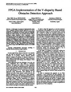
or “squashing” functions that compress an infinite input range to a finite output range, e.g. [−1, +1], see [4]. Neural networks can be “trained‘” to solve problems that are difficult to solve by conventional computer algorithms. Training refers to an adjustment of the connection weights, based on a number of training examples that consist of specified inputs and corresponding target outputs. Training is an incremental process where after each presentation of a training example, the weights are adjusted to reduce the discrepancy between the network and the target output. Popular learning algorithms are variants of gradient descent (e.g., error-backpropagation) [29], radial basis function adjustments [4], etc. Neural networks are well suited to a variety of nonlinear problem solving tasks. For example, tasks related to the organization, classification, and recognition of large sets of inputs. A. Multi-Layer Perceptron Multi-layer perceptrons (MLPs) (Fig. 1) are layered fully connected feed-forward networks. That is, all PEs (Fig. 2) in two consecutive layers are connected to one another in the forward direction. During the network’s forward pass each PE computes its output yk from the input ~ik it receives from each PE in the preceding layer as shown here: yk = ϕk (vk )
(1)
where ϕk is the squashing function of PE k whose role is to constrain the value of the local field, X vk = wkj ikj + θk (2) j
wkj is the weight of the synapse connecting neuron k to neuron j in the previous layer, and θk is the bias of neuron k. Equation 1 is computed sequentially by layer from the first hidden layer which receives its input from the input layer to the output layer, producing one output vector corresponding to one input vector. The network’s behavior is defined by the values of its weights and bias. It follows that in network training the weights and biases are the subjects of that training. Training is performed using the backpropagation algorithm after every forward pass of the network.
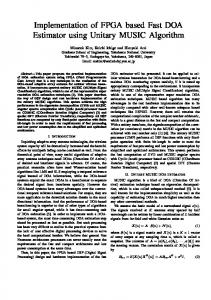
Fig. 2.
Processing element.
The network uses the error to adjust the weights in an effort to let the output yj approach the desired output dj . Back-propagation minimizes the overall network error by calculating an error gradient for each neuron from which a weight change 4wji is computed for each synapse of the neuron. The error gradient is then recalculated and propagated backwards to the previous layer until weight changes have been calculated for all layers from the output to the first hidden layer. The weight correction for a synaptic weight connecting neuron i to neuron j mandated by backpropagation is defined by the delta rule: ∆wji = ηδj yi (3) where η is the learning rate parameter, δj is the local gradient of neuron j, and yi is the output of neuron i in the previous layer. Calculation of the error gradient can be divided into two cases: for neurons in the output layer and for neurons in the hidden layers. This is an important distinction because we must be careful to account for the effect that changing the output of one neuron will have on subsequent neurons. For output neurons the standard definition of the local gradient applies. δj = ej ϕj 0 (vj ) (4) For neurons in a hidden layer we must account for the local gradients already computed for neurons in the following layers up to the output layer. The new term will replace the calculated error e since, because hidden neurons are not visible from outside of the network, it is impossible to calculate an error for them. So, we add a term that accounts for the previously calculated local gradients: X δj = ϕj 0 (vj ) δk wkj (5) k
Fig. 1.
Multi-layer Perceptron model.
B. Back-Propagation Algorithm The backpropagation learning algorithm [29] allows us to compute the error of a network at the output, then propagate that error backwards to the hidden layers of the network adjusting the weights of the neurons responsible for the error.
where j is the hidden neuron whose new weight we are calculating, and k is an index for each neuron in the next layer connected to j. As we can see from (4) and (5), we are required to differentiate the activation function ϕj with respect to its own argument, the induced local field vj . In order for this to be possible, the activation function must of course be differentiable. This means that we cannot use non-continuous activation functions in a backpropagation based network. Two continuous, nonlinear activation functions commonly used in backpropagation networks are the logistic function: ϕ (vj ) =
1 1 + e−avj
(6)
4
and the hyperbolic tangent function: ϕ (vj ) =
avj
−avj
e −e . eavj + e−avj
(7)
Training is performed multiple times over all input vectors in the training set. Weights may be updated incrementally after each input vector is presented or cumulatively after the training set in its entirety has been presented (1 training epoch). This second approach, called batch learning, is an optimization of the backpropagation algorithm designed to improve convergence by preventing individual input vectors from causing the computed error gradient to proceed in the incorrect direction.
note, this study is limited to implementation of feed-forward MLP with backpropagation learning algorithm. Also, design parameters like number of layers, number of neurons, inputoutput sizes, types of interconnection, etc are limited by the hardware resources available, depending on the type of FPGA used. There are no general rules. One has to derive the limits by experiments. Later on in this paper, we would present some statistics on the variations of these design parameters over hardware resource utilizations. Similar statistics for different platforms are also reported in [18],[19].
IV. H ARDWARE IMPLEMENTATION A. Design Architecture Our design approach is characterized by the separation of simple modular functional components and more complex intelligent control oriented components. The functional units consist of signal processing operations (e.g., multipliers, adders, squashing function realizations, etc.) and storage components (e.g., RAM containing weights values, input buffers, etc.). Control components consist of state machines [16] generated to match the needs of the network as configured. During design elaboration, functional components matching the provided parameters are automatically generated and connected, and the state machines of control components are tuned to match the given architecture. Network components are generated in a top-down hierarchical fashion as shown in Fig. 3. Each parent is responsible for generating its children to match the parameters entered by the user prior to elaboration and synthesis. Using VHDL generated statements and a set of constants whose values are given by the user configuration, the top level ANN block generates a number of layer blocks as required by the configuration. Each layer subsequently generates a teacher if learning is enabled along with a number of PEs as configured for that layer. Each PE generates a number of MACC blocks equal to the width of the previous layer as well as a squashing function block. Fig. 3 shows that there is an one-to-one relationship between the logical blocks generated (e.g., Layers, PEs, MACCs) and the functions and architecture of the conceptual ANN model. This approach has been chosen over one in which logical blocks are time-multiplexed to allow for a high-performance fully-pipelined implementation at the cost of greater resource demands. In this context, it is interesting to note how it is done at PC-based system. Fig. 4 shows the graphical user interface to generate different networks using the MATLAB Neural Network toolbox [13]. As shown in Fig. 4, one can choose network type (feed-forward backpropagation, MLP, radial basis, etc), number of layers, number of neurons per layer, the transfer functions, etc. With these inputs, the network structure is generated. Of course, one gets higher flexibility in terms of data precision, network size, etc in PC-based ANN designs. Nevertheless, we wanted to have the same flexible design philosophy for the FPGA-based design. Please
Fig. 3. Block view of the hardware architecture. Solid arrows show which components are always generated. Dashed arrows show components that may or may not be generated depending on the given parameters.
Fig. 4. Graphical user interface to generate networks in MATLAB Neural Network toolbox [13].
5
B. Data Representation Network data is represented using a signed fixed point notation. This is implemented in VLSI hardware description language (VHDL), with the IEEE proposed fixed point package [30]. Fixed point notation serves as a compromise between traditional integer math and floating point arithmetic, the latter being prohibitively costly in terms of hardware [31]. Our network has a selectable data width which is subdivided into integer and fractional portions. For example, our implementation incorporates one sign bit (S), one integer place (I), and three fractional places (F ): SI.F F F . The network data precision thus becomes 2−F (0.125 in our example) where F is the number of fraction bits and gives the data set D a maximum range of −2N −1 ≤ D ≤ 2N −1 − 2−F
(8)
(−2 ≤ D ≤ 1.875 in our example) where N = 1 + I + F is the total data width, I = 1, F = 3 for our implementation. C. Processing Element An effort was made to keep the realization of a single PE as simple as possible. The motivation for this was that in our parallel hardware design many copies of this component would be generated for every network configuration. So, keeping this component small helps to minimize the size of the overall design. The control scheme was centralized external to the PE component to prevent the unnecessary duplication of functionality and complexity. In paring the design of the PE component down to its essential features, we are left with a multiply-accumulate function with a width equal to the number of neurons in the previous layer, the selected squashing function implementation, and memory elements such as registers contained the synaptic weights and input buffers. The PE is described by (1 & 2). The full calculation of the PE is shown in Fig. 5. In Fig. 5, the MACC units multiply and sums the P inputs i with the weights w and the bias θ, to implement wkj ikj + θk as in (1 & 2). After that, the j
final quantity from the MACC is passed through the squashing function ϕ (see top right corner) to produce the network output y. As indicated in Fig. 5, the squashing function ϕ utilizes lookup table (LUT) (via ‘lut en’ instruction), described below. D. Squashing Function The direct implementation of the preferred nonlinear squashing, e.g. the sigmoid function (see eqs. 6 & 7), presents a problem in hardware since both the division and exponentiation operations require an inordinate amount of time and hardware resources to compute. The only practical approach in hardware is to approximate the function [20],[32]. But, in order for training to converge or for us to obtain accurate offline results, a minimum level of accuracy must be reached [33]. More accurate approximations will result in faster, better convergence, hence more accurate results. There has been a
Fig. 5.
Functional blocks of the PE component.
significant amount of research into how a sigmoid function can be efficiently approximated in hardware while maintaining an acceptable degree of accuracy and the continuity required for reliable convergence in backpropagation learning [32]. To create a generalized design we must add one additional requirement for sigmoid function approximation, that the method of approximation must be valid for a variety of sigmoid functions. Based on size and accuracy requirements to be met by the network we are generating, we may select one of two implementation styles for a sigmoid function that we have implemented in our generalized design: a uniform LUT or a LUT with linear interpolation, described below. Comparative analysis of the hyperbolic tangent squashing function implementation, using LUT and piece-wise linear approximation techniques are discussed in [20]. Gadea et al. compared performances of different types of implementation of squashing function in [18]. LUT-based approach works much faster than piece-wise linear approximation, though LUT consumes memory. So, if there is not much concern about memory, LUT is preferred, as in our implementations, and real-time applications, e.g., motion control and fault diagnosis of induction motor drive [25]. 1) Uniform Lookup Table Implementation: A uniform LUT implemented in block RAM may be used to approximate a function of any shape. The LUT is addressed using the local field. The address is formed by taking the inverse of the sign bit of the local field and concatenating the most significant bits required to represent the highest input value of the function mapped onto the LUT down to the number of address bits of the LUT. Altogether, the computation requires one cycle and minimal hardware to hold the table itself. The uniform LUT implementation, despite being popular in FPGA based ANNs and while efficient in terms of speed and size, presents a problem in terms of its size vs. accuracy tradeoff when it comes to modeling functions with steep slopes
6
like a sigmoid function. As the slope increases so does the quantization error between LUT entries (Fig. 6). A common solution for this problem is the use of a LUT with variable resolution (Fig. 6c). That is, a LUT with higher resolution for portions of the function with steeper slopes. However, this is a solution that must be custom crafted for every given sigmoid and thus is not easily generalized as we would like.
Fig. 7. The hyperbolic tangent function is approximated by finding the nearest indices of the LUT corresponding to the local field, then drawing a line between the values referenced by those indices. The quantization error is then used to find the corresponding point on the line segment LUT(d)LUT(d + 1).
The algorithm flow is controlled by a state machine inside the squashing function component enabled by the network controller. After receiving input, the result is registered at the output after 5 clock cycles. An analysis of the tradeoff between the hardware cost, performance, and accuracy related to this method is given in section V-A.
the error calculation of its successor. Because of this, the training algorithm must be computed sequentially, layer by layer limiting parallelism to the neuron level. The hardware implementation once again seeks to separate control and functional based components. Each layer contains its own backpropagation teacher component which is responsible for the control flow of the algorithm for its layer. Because the backpropagation algorithm is only being executed for one layer at a time we need only one set of the necessary arithmetic components. Since the number of multipliers and adders, and the size of the MACC are dependent on the size of a given layer and its predecessor, we must compute and generate the worst case number of arithmetic components that are needed during elaboration of the given network design. The set of arithmetic components used in the backpropagation calculation are then packaged into the BP ALU component. The BP ALU is accessed by each backpropagation teacher via an automatically generated multiplexer (Fig. 8) which is controlled by the network controller. To optimize the performance of the training algorithm we begin execution during the forward pass of the network. In the forward pass we are able to compute two elements of the algorithm: η~i once a given layer receives its input, and ϕ0 (v) once the layer’s output has been computed. In the hidden layers, the results of these preprocessing steps are then saved until the error gradient reaches them in the backward pass. The output layer teacher continues immediately by calculating the output error and the local error gradient (4) for every neuron in the output. Once the error gradient has been calculated at the output layer, the final hidden layer may calculate its own error gradient (5) and pass that back. Synthesis example of BP algorithm for a realistic application case would be presented in section VI-B.
E. Back-Propagation Computation
F. Network Controller
The backpropagation algorithm (see sect. III-B) relies on the calculation of the network error at the output layer to estimate the error of neurons in the previous layers. The error is estimated and propagated backwards layer by layer until the first hidden layer is reached. It follows that the error estimation of any given layer except the output layer is dependent on
The design of the network controller was strongly guided by the highly generalized design of the network and the initial decision to separate functional and control units. The decision to centralize control of the network was based on the goal of minimizing the size and complexity of components that must be generated multiple times. This is contrary to a distributed
Fig. 6. (a) Sigmoid function implemented on a uniform LUT. (b) Uniform LUT error distribution for a sigmoid function. (c) Example of partitioning for a variable resolution LUT.
2) Lookup Table With Linear Interpolation Implementation: To address the diminished accuracy of a uniform LUT while maintaining generalizations over a variety of functions, we incorporate linear interpolation alongside the LUT. This solution effectively draws a line between each point of a uniform LUT as in Fig. 7. The resulting activation function is LUT(d + 1) − LUT(d) qe + LUT(d) (9) 2N −M where LUT(d) is the value returned by a uniform LUT representing the target function for index d (done as described in section IV-D.1), N is the bit widths of the local field, M is the bit width of the LUT address bus, and qe is the quantization error described by: y=
qe = ϕ(v) − LUT(d)
(10)
7
network controller state machine (see Fig. 9).
Fig. 8.
Backpropagation implementation.
control mechanism made up of independent components capable of determining their own state and communicating that state to one another. This would be the more modular solution, but would also inflict a significant time and hardware penalty caused by the control overhead in the network, since control mechanisms would be repeated many times through the network. The centralized control scheme on the other hand, relies on the predictability of the timing and behavior of any generated network configuration. Depending on the network to be generated, the network controller is created as either an online or offline network controller. Here, offline indicates that a network is pre-trained, and then the network object is used on test data, without any training capability. This type of network is often used in hardware implementations due to less implementation complexity. On the other hand, online indicates that the network has dynamic training capability. For different applications, the network with different architecture, would train itself following particular training methods, e.g., backpropagation, before acting on test data. This provides a generalized flexibility, however, it is complex to implement. Different implementations are necessary since in offline mode a pipelined network is generated and the online controller must include control for the computation of the backpropagation algorithm. Despite this, both controllers are implemented in the same manner. The network controller is a Mealy state machine (see Fig. 9) based on a counter indicating the number of clock cycles that have passed in the current iteration (in the case of an online network) or the total number of clock cycles passed (in the case of an offline network). As mentioned above, for online application, we would need network with learning capability. It is to be noted that, for backpropagation learning algorithm, the error needs to be fed back. Therefore, Mealy state machine is suitable, as it is a finite state transducer that generates an output based on its current state and input. For the value of the counter to have any meaning we must be able to precalculate the latency to reach milestones in the forward and back passes of the network. These milestones are calculated during elaboration of the design. Based on these milestones the state machine outputs a set of enable signals to control the flow of the network. In comparison, for offline applications, one would not require training, hence the back passes in the
Fig. 9.
State machines for network controller.
V. E XPERIMENTAL R ESULTS To evaluate our system we implement a basic sample application in a varied set of configurations. To speed the process, we carried out testing using Mentor Graphics’ ModelSim simulator. A similar network implementation built using the MATLAB Neural Network Toolbox [13] is used as a basis for comparison. For comparison we take as metrics the root mean square error (RMSE) of the ANNs when applied to a test data set after 50, 100, 200, 400, and 800 epochs. We define the RMSE as: s P 2 (y − yd ) erms = (11) n where y is the calculated output of the network, yd is the desired output, and n is the number of input sets presented. A speed comparison is not meaningful due to the dubious nature of any resulting measure considering the external factors affecting execution time on a PC. We will also remark here on the results of our squashing function approximation method using a LUT combined with linear interpolation. A. LUT with Linear Interpolation To judge the accuracy of our approximation technique for sigmoid function using a LUT with linear interpolation we calculated the average error and worst case error of the technique for a range of network data precisions and LUT sizes. Using a uniform LUT as a control, we approximated the hyperbolic tangent with input ranging [-4:4]. Table I shows the worst case error using the two techniques and Table II the average error. From the results we see that the LUT with linear interpolation provides a significant improvement in accuracy. For example, in a case of a network that uses 15-bit fractional precision, an 8192 element uniform LUT can be replaced by a 128 element LUT with linear interpolation and achieve a slightly better quality approximation on average.
8
Using the LUT with linear interpolation it becomes possible to reduce the error such that the magnitude of the error falls under the resolution of the network data precision. At this point we have reached a maximally precise approximation for the given network. Table III shows the resolution necessary to register the approximation error in the worst case for each set up in our tests. The boxed entries show the minimum LUT size for a given network data resolution to reach a maximally precise approximation. The logarithmic scale on the x-axis of Table III is with base 2. This is done because number of elements in optimal LUTs in hardware always have a base 2 logarithm and because only these values are used, the step size is defined this way. This means that 10 corresponds to 210 = 1024 elements (the reason this is optimal is that to address 1024 elements, exactly 10 bits are used). Likewise, a bit resolution of −10 is equivalent to a resolution of 2−10 = 0.0009765625. −10 represents the binary place, i.e., 10 places after the decimal point. The purpose of the Table III is to show for a given data precision in the network, what the optimal size for a LUT implementing a maximally accurate standard sigmoid function is. Maximally accurate is defined by a worst case error that is less than the precision of data propagating through the network. The contents of Table III are based on Table I which describes the minimum bit precision needed to resolve the worst case error. The boxed elements in Table III give the minimum size LUT necessary to achieve a worst case error less than the resolution of the network. For example, if we consider the top left boxed entries in Table I, which have a worst case error of 3.8e − 4, the bit resolution as per Table III, must be at least −12 (2−12 = 2.4e − 4). Based on this, we can say that a lin-LUT of size 27 is the smallest size LUT that gives a maximally accurate result for a network fractional precision of 10 or 11. TABLE I W ORST CASE ERROR OF APPROXIMATED HYPERBOLIC TANGENT LUT WITH LINEAR INTERPOLATION AND A UNIFORM LUT
FUNCTION USING A
B. Spectrometry Application Our test application attempts to draw out conclusions from the frequency spectrum returned by a spectrometer. In this case we are analyzing several cuts of meat to determine the fat
TABLE II AVERAGE ERROR OF APPROXIMATED HYPERBOLIC TANGENT FUNCTION USING A LUT WITH LINEAR INTERPOLATION AND A UNIFORM LUT
TABLE III B IT RESOLUTION REQUIRED TO RESOLVE THE WORST CASE APPROXIMATION ERROR
concentration of each. The network is provided with the magnitudes of 10 principle components of detected frequencies and is trained at the output using the measured fat concentration of the cut [34]. NNs are increasingly used as a nonlinear modeling tool for spectra calibration [35], at PC-level. Here we compare the accuracy of the FPGA based implementation with that of a similar MATLAB simulation. Both use a 10-3-1 layer configuration trained using backpropagation. That is, 10 non-computing neurons in the input layer corresponding to the 10 principle components, 3 neurons in the hidden layer, and 1 output neuron corresponding to the fat concentration. The MATLAB simulation employs batch learning with a learning rate of 0.05 while our system uses incremental learning with a learning rate of 0.1. The networks are trained over 200 input/target pairings, the final 40 pairings are used for testing to evaluate the network’s ability to generalize. Input values were normalized between -2 and 2 and target values between -1 and 1. Both networks use the same initial set of weights randomized between -2 and 2. Table IV compares the RMSE of the test cases (not included in training) for the MATLAB and FPGA implementations over different number of training epochs. Comparison of performances for unseen test cases demonstrate the generalization capability of the networks. FPGA implementations use data
9
widths with 1 sign bit, 2 integer bits, and fractional data precisions of varying size (the total data width of the network data is given in the left column). The FPGA based implementations utilize LUTs with linear interpolation of the size required for maximally precise approximations as indicated in Table III. From Table IV, we can notice, the best RMSE using the MATLAB implementation for the testset is 2.63 (obtained using 800 training epochs). In comparison, the FPGA implementation achieves the best testset RMSE of 3.05 (for 18-bit data width, using 400 training epochs). Expectedly, FPGA implementation results in less accuracy compared to PC-based implementation using MATLAB, possibly due to factors like limitation in data width, fixed point data precision, incremental learning instead of batch learning, etc. However, the best performance of the FPGA implementation is reasonably acceptable compared to that of MATLAB. Also, in the FPGA implementation of the online network, we could flexibly parameterize data widths, number of training epochs, etc, a central aim of this study. TABLE IV RMSE OVER THE TEST SET Epoch
50 10.62
MATLAB 100 200 9.86 7.09
400 4.33
800 2.63
400 10.56 3.09 3.05
800 10.56 3.44 3.09
FPGA Epoch 8-bit 12-bit 18-bit
50 9.39 5.04 4.78
100 10.56 4.47 4.23
200 10.56 3.96 3.63
A maximally precise approximation however is not always necessary for a functional network. In [32] Tommiska regards a maximum error of 0.0039 to be the functional limit on the accuracy of the squashing function for network training, and a maximum error of 0.0078 as the limit for the forward pass. Table V compares the RMSE over the test set of two FPGA implementations of networks with 12-bit data precision, one implemented with a 64-element LUT with linear interpolation and one with a uniform 64-element LUT. We see that indeed the network is still functional as Tommiska predicts. However, training becomes noticeably erratic and the accuracy of the network is significantly diminished as expected. TABLE V RMSE OF AN FPGA
BASED NETWORK WITH SQUASHING FUNCTIONS IN
THE HIDDEN LAYER IMPLEMENTED USING A
LUT WITH LINEAR
INTERPOLATION AND THE SAME NETWORK IMPLEMENTED USING UNIFORM
Epochs Lin-LUT Uni-LUT
50 5.04 4.75
100 4.47 4.95
LUT S 200 3.96 4.35
400 3.09 4.53
800 3.44 3.70
VI. D ISCUSSION Ideally, we would like to make accuracy and performance comparisons only against other hardware based systems. This is for two reasons. First, hardware based ANNs allow for
more meaningful measures of computation time. In software — particularly software in a PC environment — computation time is affected by a series of external factors such as the characteristics of the processor and the current load on the system. Second, software based ANNs are able to employ a number of features that may not be practical or feasible in hardware such us floating point notation or advanced training techniques. Software and hardware based ANNs are two very different creatures. Hardware in general — but not in all cases — tends to lend itself to faster performance. But, it is less capable of utilizing more complex techniques to achieve a higher degree of accuracy as software is able to. This disparity reduces the value of such comparisons since in reality we are comparing two significantly different networks. However, considering the scarcity of backpropagation ANN networks in hardware, and without access to training and test data for those few ANNs, the MATLAB Neural Network Toolbox [13] remains a viable alternative benchmark for accuracy when care is taken to note the inequities inherent in the comparison. On the other hand, we are able to make performance comparisons against other hardware platforms using a set of standard performance metrics. This comparison will be presented in section VI-B. A. System Accuracy We found that in our sample application, the FPGA based network converges over fewer iterations than the MATLAB simulation. This comes as a result of incremental learning and a higher learning rate. The quality of the FPGA based network’s convergence however, is not as good. The FPGA based network must utilize a higher learning rate to reduce the increased chance of the training algorithm becoming trapped in a local minimum as a result of using incremental learning. This in turn causes the overall network error gradient to become unstable earlier in training; a symptom of overshooting the target value in training. The MATLAB simulation on the other hand, is less likely to overshoot a target in training thanks to its low learning rate and is at the same time less likely to become trapped in local minima using batch learning. The extremes of the target output are other contributors to the error in the FPGA implementation. The range of the calculated output does not reach the extreme ends of the target range. This is attributed to the eventual averaging of the weight changes caused by changes to the error gradient for each iteration in training. This sample application proved to be a somewhat special case. In testing we found that we could train the network for an unusually large number of epochs without experiencing any overfitting in the test set. We found that the error in the test set bore a strong relation to the training set error in both implementations. In this sample application we never saw the expected divergence caused by over training the network. This occurs when data sets contain few if any outliers, the training set is very representative of the relation, and the test set conforms well to that relation. Given a larger, more diverse test set or a smaller training set, we expect to observe a divergence between error of the training set and that of the test set.
10
From Table IV it is clear that the data precision of the ANN plays an important role in the network’s ability to converge in training and its resulting accuracy. Our own testing seems to show that Holt and Hwang’s assertion [33], that 13 bits is the minimum required precision for network weights and biases to reliably obtain convergence using backpropagation learning, is not a firm rule. We found that our 12-bit implementation can still yield a successful convergence, while indeed, lower bit widths like that of our 9-bit implementation results in rather poor convergence. The unexpected success of the 12-bit implementation is likely due in part to the expansion of the data path for intermediate results in our network. B. Hardware Implementation To measure the performance of ANNs across the wide range of platforms that they have been implemented on, there are two common criteria: connections per second (CPS) and connection updates per second (CUPS). CPS is defined as the number of multiply-add operations that occur in the forward pass of a network per second. CUPS is the number of weight updates per second in the network. Two additional derivations of these metrics exist. First, to account for the number of connections in the network that must be computed or updated we may calculate connections per second per weight (CPSPW) or connection updates per second per weight (CUPSPW). Secondly, we may take into account the precision of the network by calculating the connection primitives per second (CPPS) or the connection primitives per second per weight (CPPSPW) to account for both the number of connections in the network and the precision of the network data [38]. Table VI presents a performance comparison between our network and other implementations using these metrics. The performance data of our network reflects the 12-bit implementation of the spectrometry application presented earlier in section V-B. Due to the parallel implementation of FPGA based neural networks like ours and the implementation presented in [17], the CPS metric increases as a function of the number of synaptic connections. This is because as more neurons are implemented in parallel, more MACC operations can occur simultaneously, thereby increasing the number of operations per second. The CPSPW metric is a means for normalizing this behavior by dividing by the number of weights. However, in parallel implementations, this metric punishes networks with wide input vectors by including weights in the normalization that are not connected to multiply-add operations on the input side. The implementation of our system maximizes flexibility and parallelism over hardware cost. This is seen for example in that when a squashing function implementation for a layer of PEs requires a LUT, each PE is given a dedicated LUT as opposed to sharing it with other PEs. We do this to allow each PE the potential to have its own squashing function, implementation type, and level of accuracy. As a result of choices to maximize flexibility, network designs generated on our platform are likely to be somewhat larger than any application specific designs.
Parallelism in the network is implemented at the synaptic level, this represents the maximum level of parallelism for neural networks. Using synaptic level parallelism, all neurons and synaptic connections in a network layer operate in parallel with the goal of maximizing performance. Performance in the offline network is further improved with the use of a fully pipelined design. TABLE VI A COMPARISON OF ANN PLATFORMS AND IMPLEMENTATIONS Platform Our FPGA (offline) Our FPGA (online) FPGA [17] (offline) FPGA [17] (online) ETANN [36] LNEURO [7] CNAPS [37] Virtex XCV400 (pipeline) [19] Virtex XCV400 (non pipeline) [19] X2V8000 (pipeline) [18] FPNA [21] XC4003 [22] XC3090 [23]
CPS 536M 140M 597M 250M 2.0G 100M 1.6G 81M
CPSPW 16.2M 4.24M 37.3M 41.7M 200K 100K 6.1K -
CPPS 77.2G 20.2G 72G 6.4G 102G -
CPPSPW 2.34G 612M 7.0M 6.4M 400K -
CUPS 106M 81M
81M
-
-
-
17M
4.65G
-
-
-
4.65G
200M 22M 2M
-
-
-
25M 0.1M
As an example of the hardware resource demands of a network generated using our system, we take the online implementations of the 12-bit spectrometry application network. Table VII shows the quantities of selected components generated during synthesis to implement the networks of different sizes as well as the total percentage of area consumed against the available resources on the Virtex-5 xc5vsx50t-2ff1136 platform [28]. The amount of hardware resources consumed by a network implemented using our platform is strongly influenced by many factors. The two most influential of these factors are the dimensions (governed by network structure) and the data width of the network. Naturally, as shown in Table VII, networks of greater size result in greater hardware requirements. The structure 10-3-1 has been used for the results shown in Tables IV & V. For brevity purpose, networks of lower sizes are not shown. Besides, parallel calculation of the backpropagation makes consecutive wide layers especially costly, requiring a number of MACCs equal to the product of the width of the two widest consecutive layers. When choosing the data width of the network, careful consideration should be made to match the data width to the width of hardware arithmetic units on the target FPGA. Wider data widths than the width of hardware arithmetic units necessitate additional sets of those units to implement the design, thereby significantly increasing the final hardware requirements of the implementation. Examples of hardware resource consumptions in other neural network implementation and applications, reported by the synthesis results of various works, are briefly shown in Table VIII. It is to be noted that Table VIII employs many different network structures for various applications. Hence, it should not be used as a direct comparison to Table VII.
11
TABLE VII H ARDWARE RESOURCE UTILIZATION IN 12- BIT SPECTROMETRY APPLICATION USING X ILINX XC 5 VSX 50 T-2 FF 1136
TABLE VIII R ESOURCES USED IN DIFFERENT NN IMPLEMENTATION AND APPLICATIONS Ref [18] [18] [18] [19] [24]
Platform Virtex II X2V250 XCV300 Virtex II X2V8000 Virtex XCV400 Virtex 4 LX25
ROM
10
4 Input LUT 1931 3713 81895 5925 7748
Nevertheless, there are probably no parametric rules to estimate how network implementation in FPGA scales up. Therefore, the statistics on hardware resource utilizations from the synthesis reports, as shown in Table VII & VIII, should be used to estimate hardware demands (for specific platforms) with growing network structure. Of course, for a particular platform, there would be resource limitation, putting constraints on the upper limit of the possible network size. However, a rough overview on the possible hardware requirements, e.g., in Tables VII and VIII, could be a rough guide in choosing the appropriate FPGA platform for any particular application and network structure requirements. C. Future Directions Some interesting additions could bring the accuracy of this hardware based network implementation closer to that of software based ones. The first step in this direction would include the implementation of a momentum factor in the backpropagation training algorithm. The momentum factor speeds learning and brings us to a better convergence by rewarding training that consistently reduces error and punishes any increases in error. This could not be covered in this work mainly because of hard time-limits for the thesis. A second more complex step is the implementation of batch learning. Batch learning is a common approach in software based implementations, and as we saw in section V-B, effective in finding good convergence. When combined with a momentum factor, batch learning is particularly adept at fast and accurate convergence. The implementation of batch learning on an FPGA platform faces challenges in either calculating intermediate weights quickly enough in order not to cause buffering of the weight array and network output, or, implementing external memory to buffer the necessary data without slowing the system to the point that a software based solution becomes a better choice. Because of our primary interest to implement and test ANN with learning on FPGA, we skipped real-time input data communication to the FPGA, which would have required considerable effort to design such communication module. Such real-time online input data feeding is important to check how fast the FPGA can process new data. However, that is
Slices 1299 2519 46590 3473 5971
Flip flop 846 896 17454 786 9061
MACC 24
Bonded IOB
168 44 140
somewhat dependent on the clock frequency of the FPGA platform, not the direct focus of this work. This would be part of the future work, where we plan to test the ANN implemented in FPGA with real-time input data communication. VII. C ONCLUSION In this paper, we have presented the development and implementation of a parameterized FPGA based architecture for feed-forward MLPs with backpropagation learning algorithm. Our architecture makes native prototyping and design space exploration in hardware possible. Testing of the system using the spectrometry sample application showed that the system can reach 530 million connections per second offline and 140 million online. These speeds represent comparable performance to other hardware based MLP implementations. We have also confirmed that our system is capable of producing accurate convergence in training on a par close to MATLAB simulations. Statistics on hardware resource utilizations from the synthesis reports of different network sizes are presented. These could be used to estimate hardware demands (for specific platforms) with growing network structure. Also presented was a new method for approximation of a sigmoid function in hardware. We showed that by applying a linear interpolation technique to a uniform LUT, we could significantly reduce the size of the necessary LUT while maintaining the same degree of accuracy at the cost of implementing one adder and one multiplier. ACKNOWLEDGMENTS This paper is based on work carried out by Alexander Gomperts at ABB Corporate Research, Switzerland from September 2008 to February 2009 under the supervision of Abhisek Ukil and Franz Zurfluh in partial fulfillment of the requirements of a Master’s of Electrical Engineering degree from the Technische Universiteit Eindhoven, The Netherlands. Supervision on the side of the University was provided by Lech J´oz´ wiak. An internship preceded this thesis work. The authors would like to thank the anonymous reviewers for the constructive review, helping to upgrade the paper.
12
R EFERENCES [1] I. A. Basheer and M. Hajmeer, “Artificial neural networks: fundamentals, computing, design, and application,” Journal of Microbiological Methods, vol. 43, pp. 3–31, Dec. 2000. [2] M. Paliwal and U. A. Kumar, “Neural networks and statistical techniques: A review of applications,” Expert Systems with Applications, 2008. [3] B. Widrow, D. E. Rumelhart, and M. A. Lehr, “Neural networks: applications in industry, business and science,” Communications of the ACM, vol. 37, no. 3, pp. 93–105, 1994. [4] A. Ukil, Intelligent Systems and Signal Processing in Power Engineering. New York: Springer, 1st ed., 2007. [5] B. Schrauwen, M. D’Haene, D. Verstraeten, and J. V. Campenhout, “Compact hardware liquid state machines on FPGA for Real-Time speech recognition,” Neural Networks, vol. 21, no. 2-3, pp. 511–523, 2008. [6] C. Mead and M. Mahowald, “A silicon model of early visual processing,” Neural Networks, vol. 1, pp. 91–97, 1988. [7] J. B. Theeten, M. Duranton, N. Mauduit, and J. A. Sirat, “The LNeuro chip: A digital VLSI with on-chip learning mechanism,” in Proc. Int. Conf. on Neural Networks, vol. 1, pp. 593–596, 1990. [8] J. Liu and D. Liang, “A survey of FPGA-Based hardware implementation of ANNs,” in Proc. Int. Conf. Neu. Net. Brain, vol. 2, pp. 915–918, 2005. [9] P. Ienne, T. Cornu, and G. Kuhn, “Special-purpose digital hardware for neural networks: An architectural survey,” The Journal of VLSI Signal Processing, vol. 13, no. 1, pp. 5–25, 1996. [10] A. R. Ormondi and J. Rajapakse, “Neural networks in FPGAs,” in Proc. Int. Conf. on Neural Information Processing, vol. 2, pp. 954–959, 2002. [11] B. J. A. Kroese and P. van der Smagt, An Introduction to Neural Networks. The University of Amsterdam, 4 ed., Sept. 1991. [12] J. Zhu and P. Sutton, “FPGA Implementations of Neural Networks - A Survey of a Decade of Progress,” Lecture Notes in Computer Science, vol. 2778/2003, pp. 1062–1066, 2003. [13] The MathWorks Inc., “MATLAB Neural Network Toolbox user guide, ver. 5.1,” Natick, MA, 2006. [14] A. Rosado-Munoz, E. Soria-Olivas, L. Gomez-Chova, J. V. Frances, “An IP Core and GUI for Implementing Multilayer Perceptron with a Fuzzy Activation Function on Configurable Logic Devices,” Journal of Universal Computer Science, vol. 14, no. 10, pp. 1678–1694, 2008. [15] E. Sanchez, “FPGA implementation of an adaptable-size neural network,” in Proc. Int. Conf. ANN, vol. 1112, pp. 383–388, 1996. [16] A. R. Ormondi and J. Rajapakse, FPGA Implementations of Neural Networks, New York: Springer, 2006. [17] N. Izeboudjen, A. Farah, H. Bessalah, A. Bouridene, and N. Chikhi, “Towards a Platform for FPGA Implementation of the MLP Based Back Propagation Algorithm,” Lecture Notes in Computer Science, vol. 4507/2007, pp. 497–505, 2007. [18] R. Gadea, R. C. Palero, J. C. Boluda and A. S. Cortes, “FPGA implementation of a pipelined on-line backpropagation,” The Journal of VLSI Signal Processing, vol. 40, pp. 189–213, 2005. [19] R. Gadea, J. Cerda, F. Ballester, A. Mocholi, “Artificial neural network implementation on a single FPGA of a pipeline on-line backpropagation,” in Proc. Int. Symp. on System Synthesis, pp. 225–230, 2000. [20] P. Ferreiraa, P. Ribeiroa, A. Antunes and F. M. Dias, “A high bit resolution FPGA implementation of a FNN with a new algorithm for the activation function,” Neurocomputing, vol. 71, pp. 71–77, 2007. [21] B. Girau, “Building a 2D-compatible multilayer neural network,” in Proc. Int. Joint Conf. on Neural Networks, pp. 59–64, 2000. [22] S. L. Bade and B. L. Hutchings, “FPGA-based stochastic neural network implementation,” in Proc. IEEE Workshop on FPGAs for Custom Computing Machines, pp. 189–198, 1994. [23] J. G. Elredge and B. L. Hutchings, “RRANN A hardware implementation of the backpropagation algorithm using reconfigurable FPGAs,” in IEEE World Conf. Computational Intelligence, pp. 77–80, 1994. [24] G. Alizadeh, J. Frounchi, M. B. Nia, M. H. Zariff and S. Asgarifar, “An FPGA implementation of an artificial neural network for prediction of cetane number,” in Int. Conf. Comp. Comm. Engg., pp. 605–608, 2008. [25] S. Tatikonda and P. Agarwal, “Field programmable gate array (FPGA) based neural network implementation of motion control and fault diagnosis of induction motor drive,” in IEEE Conf. Ind. Tech., pp. 1–6, 2008. [26] A. Mellit, H. Mekki, A. Messai and H. Salhi, “FPGA-based implementation of an intelligent simulator for stand-alone photovoltaic system,” Expert Systems with Applications, vol. 37, pp. 6036–6051, 2010. [27] A. Rahnamaei, N. Pariz, A. Akbarimajd. “FPGA implementation of an ANN for detection of anthelmintics resistant nematodes in sheep flocks,” in Proc. IEEE Conf. Ind. Electronics Applications, pp. 1899–1904, 2009. [28] Xilinx,“Virtex-5 FPGA user guide,” 2007.
[29] D. E. Rumelhart, G. E. Hinton, and R. J. Williams, “Learning internal representations by error propagation,” Nature, vol. 323, pp. 533–536. newblock MIT Press, 1986. [30] D. Bishop, “Fixed point package.” http://www.eda.org/vhdl-200x/vhdl200x-ft/packages/fixed pkg.vhd. [31] K. Nichols, M. Moussa, and S. Areibi, “Feasibility of Floating-Point arithmetic in FPGA based artificial neural networks,” in Proc. Int. Conf. Computer Applications in Industry and Engineering, 2002. [32] M. Tommiska, “Efficient digital implementation of the sigmoid function for reprogrammable logic,” IEE Proceedings Computers and Digital Techniques, vol. 150, pp. 403–411, 2003. [33] J. Holt and J. Hwang, “Finite precision error analysis of neural network hardware implementations,” IEEE Transactions Computers, vol. 42, pp. 281–290, 1993. [34] Carnegie Mellon University, “Tecator data set.” Available: http://lib.stat.cmu.edu/datasets/tecator. [35] A. Ukil, J. Bernasconi, H. Braendle, H. Buijs and S. Bonenfant, “Improved Calibration of Near-Infrared Spectra by Using Ensembles of Neural Network Models,” IEEE Sensors J., vol. 10, pp. 578–584, 2010. [36] M. Holler, S. Tam, H. Castro, and R. Benson, An electrically trainable artificial neural network (ETANN) with 10240 ”Floating Gate” synapses, pp. 50–55. IEEE Press, 1990. [37] D. Hammerstrom, “A VLSI architecture for high-performance, low-cost, on-chip learning,” in Proc. Int. Joint Conf. NN, vol. 2, pp. 537–544, 1990. [38] E. van Keulen, S. Colak, H. Withagen, and H. Hegt, “Neural network hardware performance criteria,” in IEEE World Congress on Computational Intelligence, vol. 3, pp. 1955–1958, 1994. Alexander Gomperts received his B.Sc in Electrical Engineering from the Worcester Polytechnic Institute in Worcester, MA, USA in 2004 and his M.Sc in Electrical Engineering from the Technische Universiteit Eindhoven, Eindhoven, The Netherlands in 2009. Currently, he is a hardware engineer at Satellite Services B.V. in Noordwijk, The Netherlands.
Abhisek Ukil (S’05-M’06–SM’10) received the B.E. degree in electrical engineering from the Jadavpur Univ., Calcutta, India, in 2000 and the M.Sc. degree in electronic systems and engineering management from the Univ. of Bolton, Bolton, UK. He received his Ph.D. from the Tshwane Univ. of Technology, Pretoria, South Africa in 2006. After joining in 2006, currently he is a Principal Scientist at the Integrated Sensor Systems Group, ABB Corporate Research, Baden-Daettwil, Switzerland. He is author/coauthor of more than 35 published scientific papers including a monograph Intelligent Systems and Signal Processing in Power Engineering (Springer, Heidelberg, 2007), inventor/coinventor of 6 patents. His research interests include signal processing, machine learning, power systems and embedded systems.
Franz Zurfluh received his B.Sc. in electrical engineering from the University of Applied Sciences Northwestern Switzerland, Windisch, Switzerland, in 1985. He has worked in the research and development areas for different companies mainly in the embedded electronics sector. After joining in 2000, currently he is a Principal Scientist at the Integrated Sensor Systems Group, ABB Corporate Research Center, BadenDaettwil, Switzerland. His current research interests include VLSI signal processing and control, design of FPGA-based systems for power control and automation applications.