each respective storey. As such, the EFT forces are known a priori for any ground acceleration record. As opposed to the PsD test method in which the ground ...
10.1098/rsta.2001.0879
Development and implementation of the effective force testing method for seismic simulation of large-scale structures By C a r o l K. Shield, Catherine W. F r e n c h a n d J o h n T i m m Department of Civil Engineering. University of Minnesota, 500 Pillsbury Drive SE, Minneapolis, MN 55455, USA This paper describes the development and experimental implementation of a realtime earthquake simulation test method for large-scale structures. The method, effective force testing (EFT), is based on a transformation of coordinates, in which case the structure is fixed at the base (similar to the set-up for the pseudo-dynamic (PsD) test method); however, in the case of EFT, the method is based on a force-control algorithm rather than a displacement-control algorithm. Effective forces, equivalent to the mass of each storey level multiplied by the ground acceleration, are applied at each respective storey. As such, the EFT forces are known a priori for any ground acceleration record. As opposed to the PsD test method in which the ground displacements to be imposed are affected by the measured structural response as the stiffness changes. As in the case of the PsD test method, the EFT method is suitable for testing any type of structural system that can be idealized as a series of lumped masses (e.g. building or bridge structures). Research has been conducted on a linear elastic single-degree-of-freedom system at the University of Minnesota to develop and investigate implementation of the EFT method. A direct application of the EFT method was found to be ineffective because of a natural velocity feedback phenomenon between the actuator and the structure to which it is attached. A detailed model of the control, hydraulic and structural systems was developed to study the interaction problem and other nonlinear responses in the system. The implementation of an additional feedback loop using the measured velocity of the test structure was shown to be successful at overcoming the problems associated with actuator–control–structure interaction, indicating that EFT is a viable real-time method for seismic simulation studies. Keywords: seismic simulation; testing methods; effective force testing; dynamics; control requirements; large-scale testing
1. Introduction There have been three primary test methods used to investigate the performance of structural systems subjected to seismic loadings: shaking-table studies, quasistatic cyclic studies of components, and pseudo-dynamic (PsD) test methods (Moehle 1996). Each of these methods has advantages and disadvantages. For example, with shaking-table studies, test structures may be subjected to actual earthquake acceleration records to investigate dynamic effects; however, the size of the structure is Phil. Trans. R. Soc. Lond. A (2001) 359, 1911–1929
1911
c 2001 The Royal Society �
1912
C. K. Shield, C. W. French and J. Timm (a)
global reference xa xg x
(b) .. xa
x
m
k 2
m
actuator .. peff (t) = −mxg
c
k 2
k 2
.. xg
.. x
c
k 2
ground
.. .. .. mxa = mxg + mx
.. mx .. −mxg
kx 2
. cx
kx 2
kx 2
. cx
kx 2
Figure 1. Development of the EFT method: (a) support motion of SDOF system; and (b) effective force testing.
typically limited or scaled by the capacity of the shaking table. At smaller scales, it is difficult to investigate structural details including phenomena such as bond, shear and anchorage. In addition to possible scaling limitations, control problems may include undesirable pitching of the shaking table from the applied motions. Quasistatic cyclic studies of components offer the advantage of investigating actual details. However, effects associated with the dynamic nature of earthquakes are not captured in these tests. The demands on the elements may not simulate those imposed in an actual earthquake. The PsD method enables testing of large structures (details, bond, shear, anchorage), and the loading history is intended to simulate an actual earthquake. The dynamic effects, however, are difficult to simulate with the PsD test method, because a displacement-control algorithm is used. The imposed deformations are not known a priori. For this test method, the imposed displacements depend on the response of the structure due to changes in the structural stiffness as the structure becomes damaged. As researchers try to develop a near real-time PsD test method, difficulties arise as the structure generates real inertial and damping forces, already accounted for in the computational algorithm used to determine the displacements to be imposed. The effective force testing (EFT) method, described in this paper, represents a fourth type of seismic testing. The main advantage of the EFT method is the ability to perform real-time earthquake simulation on large-scale structures because the forces are known a priori.
2. Description of the EFT method The concept of the EFT method is based on a transformation of coordinates. The response of a system to a given ground motion may be replicated by applying an Phil. Trans. R. Soc. Lond. A (2001)
The effective force testing method
1913
effective force (−m¨ xg ) to each mass of the system. Figure 1a shows a single-degreeof-freedom (SDOF) system subjected to a base motion, x ¨g . The following equation of motion may be obtained for this system: m¨ xa + cx˙ + kx = 0,
(2.1)
where x is the displacement of the mass, m is the mass of the system, c is the viscous damping coefficient, and k is the system stiffness. Subscript ‘a’ refers to motion relative to a fixed reference frame (absolute displacement). Motions of the mass relative to the ground are non-subscripted. The absolute displacement of the system mass consists of the displacement of the mass with respect to the ground and the ground displacement: xa = x + xg .
(2.2)
Coordinate transformation of the acceleration results in ¨+x ¨g . x ¨a = x
(2.3)
Combining equations (2.1) and (2.3) yields m¨ x + cx˙ + kx = −m¨ xg = Peff (t).
(2.4)
For a SDOF system, the mass multiplied by the ground acceleration is equivalent to an ‘effective force’, Peff (t), applied to the mass in a fixed reference frame (Clough & Penzien 1975; Chopra 1995). The proposed technique uses the same set-up as PsD testing (i.e. the test structure is fixed to the ground, and all motions are measured relative to the ground, see figure 1b), and restrictions on the type of structure that can be tested are similar to those required by the PsD test method (i.e. structure must be idealized as a lumped mass system). The effective force (−m¨ xg ) to be applied to the structure, in the EFT method, is a function of the mass of the structure, which is typically known or can be estimated with good accuracy before testing, and the earthquake ground acceleration record to be used. Consequently, the force-control loading history (−m¨ xg ) is known a priori for any earthquake acceleration record. Theoretically, the EFT method can be applied directly to test systems with nonlinear stiffness and damping. As the structural system stiffness and damping change, the structural response will be affected, but the applied effective force should not be affected, as shown by equation (2.4). No structural parameters (stiffness or damping) are needed to determine the effective (applied) force. The extension of the effective force technique to multiple-degree-of-freedom (MDOF) systems is illustrated in figure 2. In this case, an effective force is applied to each level (lumped mass) of the structure. The forces at each level are equal to the mass at that level multiplied by the ground acceleration. Therefore, even for the case of an MDOF system, each of the applied effective storey forces are known before the test begins. The concept of EFT is not new. It has been described in papers discussing the PsD test method (Mahin & Shing 1985; Mahin et al . 1989; Thewalt & Mahin 1987). These papers presented the possibility of using a PsD test set-up with explicit time-varying forces imposed at each lumped mass to conduct real-time tests without the need for computing and imposing required displacements. Because of the lack of displacement control and required integration algorithms, the EFT technique is conceptually Phil. Trans. R. Soc. Lond. A (2001)
1914 (a)
C. K. Shield, C. W. French and J. Timm xa2 xg
x2
m2
.. xa2
(b) x2 = xa2 − xg actuator .. Peff2 = −m 2 xg
k2, c2 xg
xa1 x1
m1
.. xa1 x1 = xa1 − xg k1, c1
xg
ground
.. xg
k2, c2 actuator .. Peff1 = − m1xg k1, c1
Figure 2. Application of EFT to MDOF systems.
and physically different from ‘real-time pseudodynamic testing’ (Nakashima et al . 1992). While the testing scheme is conceptually simple, its implementation has been considered to be problematic. Thewalt & Mahin (1987) stated that the technique requires high-quality controllers and servovalves, but the total test control problem may be simpler than that of a shaking table. Although S. A. Mahin (1987, unpublished data) indicated that shaking-table testing is probably more practical given both the power supply capacity and the relative displacements required of the degree of freedom masses, the energy input to the structure would be expected to be the same for the two testing techniques for equal structural deformation response. In fact there is potential for laboratory energy and power savings for EFT, because there is no shaking table to be moved. As far as the authors know, no other researchers have performed experimental work on the EFT method. Although the implementation of the EFT method at first appears straightforward, Murcek (1996) at the University of Minnesota demonstrated that with a direct application of the method, the actuator was unable to apply the effective force near the natural frequency of the system on a linear elastic SDOF structure. The results of Murcek’s (1996) research verified conclusions drawn by Dyke et al . (1995) regarding effects of control–structure interaction; that is, for lightly damped structures, actuators have a severely limited ability to apply forces near the natural frequency of the structures to which they are attached. This inability to apply the correct force at the natural frequency of the structure is due to ‘natural’ velocity feedback of the actuator; because the actuator is attached to the test structure, the actuator piston moves according to the response of the structure to the applied force, increasing the flow required by the actuator to produce the correct force. Dimig et al . (1999) proposed a solution to the natural velocity feedback problem that comprised incorporation of an additional feedback loop to negate the natural velocity feedback of the actuator. This paper describes improvements to the control–actuator–structural model and an experimental implementation of the natural velocity feedback correction suggested by Dimig et al . (1999). Phil. Trans. R. Soc. Lond. A (2001)
1 CF
(b)
kips to volts servovalve / actuator / structure interaction model
sign
(f)
*u q max 1 − u ps
.. mxg
(a) 1 CF
controller input −
Vc
+ DC kips to volts
(c) Ve
error
gain
IL error (d) VILc VILe gain K P IL d d R (s + Pd) −
VIL f
(g) α
* product
q
1
−
C12 s + G
A
( j)
1 SF
A
s
ms2+cs+k
.
x
(k) .
x
1 x s
natural velocity feedback
(n) Vv f c
f
SDOF model
(e)
spool postion to volts
(i)
(h) p
The effective force testing method
A
Kv KIL gain velocity feedback correction
. x
(l)
(m)
R1C1 s +1
1 Rf Cf s +1
R2C2 s +1
phase adjustment
1915
Figure 3. Model of the dynamic system incorporating the nonlinear relationship describing servovalve flow with the linearized model for velocity feedback.
Phil. Trans. R. Soc. Lond. A (2001)
Vf
1916
C. K. Shield, C. W. French and J. Timm
3. Dynamic system model for a single degree of freedom with a three-stage servovalve Equations describing the system dynamics for an SDOF structure excited by a hydraulic actuator that account for actuator–structure interaction have been proposed by Merritt (1967). If the increased flow required by the actuator is supplied, it should be possible for the actuator to apply force to the system at its natural frequency. A means of supplying this correction flow is to modify the command signal to the controller, to account for the increase in flow. Figure 3 shows the dynamic system model for an SDOF structure excited by a hydraulic actuator with a threestage servovalve in force control with the proposed correction for the natural velocity feedback. A detailed derivation of the precursor to this model can be found in Dimig et al . (1999). The blocks in figure 3 are labelled with letters (a)–(n) for the purpose of describing the model. The earthquake effective force (−m¨ xg ) is the model input. Blocks (a) and (b) represent the conversions of the effective force and actuator load cell feedback signals from load to volts, respectively. The gain factor in block (c) represents the proportional gain, which was set within the controller. Block (d) represents a simplified model for the three-stage valve driver, showing the conversion from voltage to the servovalve main stage spool opening, α. Included in this transfer function is a model for a single pole valve driver, with parameter Pd , which approximates the valve dynamics by representing the time delay associated with movement of the spool (F. N. Bailey 1987, unpublished notes). The mechanical gain, Kd , represents the DC gain of the valve driver. Figure 4 is a schematic of a four-way servovalve. For this type of servovalve, the oil flow through the valve is a nonlinear function of the servovalve spool opening and the pressure across the piston is described by the following flow–pressure relationship: � α pl q =α 1− , (3.1) qmax |α| ps where q is the flow through the actuator, qmax is the maximum flow with full effective supply pressure drop across the servovalve, pl is the difference in pressure across the actuator piston, and ps is the hydraulic supply pressure. Block (f) is a representation of this relationship. Blocks (g) and (h) represent the actuator, where C12 is the oil compressibility constant, G is the sum of the actuator leakage constant and the valve leakage constant, and A is the cross-sectional area of the actuator piston (F. N. Bailey 1987, unpublished notes; Merritt 1967). The transfer function for the linear elastic test structure is shown in block (i). The velocity response of the SDOF system is integrated in block (k) to obtain the displacement response. The ‘natural’ velocity feedback is represented by block (j). The natural velocity feedback correction is shown in blocks (l)–(n). The measured velocity multiplied by the piston area is the flow which needs to be added to the actuator. Because the command signal is modified rather than the flow, all of the model parameters that convert the command voltage, Vc , to flow, q, must be used to convert the ‘correction flow’ to the correction voltage, Vvfc . Hence the measured velocity multiplied by the piston area is multiplied by an inverse of the transfer Phil. Trans. R. Soc. Lond. A (2001)
The effective force testing method
1917
functions in blocks (c)–(f) to produce the proper correction voltage: Vvfc =
A x, ˙ Kv KIL gain
(3.2)
where Kv and KIL are parameters discussed below, and ‘gain’ is the outer-loop gain setting of the controller. This voltage is then summed with the effective force voltage signal to produce the ‘corrected’ command signal, which is input to the controller. For experimental simplification, a linearized equivalent of equation (3.1) is used in the feedback correction, where the flow in the servovalve is assumed to be proportional to the spool opening, independent of the pressure across the actuator piston: q = Kv α,
(3.3)
where Kv is the null flow gain, qmax of equation (3.1). In the velocity feedback correction block (n), the factor KIL is introduced. This factor represents the overall gain applied by the inner-loop parameters in block (d), which convert the inner-loop command signal, VILc , to the valve spool opening, α: KIL =
(gainIL )(Kd /R) , 1 + (gainIL )(Kd /R)(1/SF )
(3.4)
where gainIL is the inner-loop gain setting on the controller, R is the nominal output resistance of the controller, and SF is the known conversion factor for the controller from spool opening to inner-loop voltage (VIL ). The phase adjustment incorporated into the velocity feedback correction, shown in blocks (l)–(m), was needed to offset time delays in the dynamic system, such as those explicitly modelled in the servovalve dynamics (block (d)). The lead–lag compensation network in block (l) was the primary means of adjusting the phase of the velocity feedback correction. As implemented, the magnitude and phase response of the operational amplifier lag network were given by � 1 + (ωR1 C1 )2 M (ω) = � , 2 (3.5) 1 + (ωR2 C2 ) −1 −1 φ(ω) = tan (R1 C1 ω) − tan (R2 C2 ω). The resistance and capacitance values were chosen so that the magnitude of the transfer function was near unity for all frequencies of interest, and the lag was close to offsetting the delay in the servovalve. The low-pass filter (block (m)) was provided as a means of making small, ‘fine-tune’ adjustments to the phase of the velocity signal. The filter had amplitude and phase responses given by 1 M (ω) = � , 1 + (ωRf Cf )2 (3.6) −1 φ(ω) = − tan (Rf Cf ω). The amplitude of the transfer function was near unity for the frequency range at which the system was operating. Typical values for Rf and Cf were 12 kΩ and 0.047 µF, respectively. The gain factor and phase adjustment factors described above were independent of the properties of the SDOF structure. The servovalve dynamics in block (d) and the phase adjustment in blocks (l)–(m) described further in Phil. Trans. R. Soc. Lond. A (2001)
1918
C. K. Shield, C. W. French and J. Timm α
q supply ps
p1 p = p1 − p2
q
q p2
Return po ≈ 0
q
Figure 4. Schematic of four-way servovalve.
Timm (1999) represent refinements over the model originally developed by Dimig et al . (1999). In addition, Dimig et al .’s model was based on a two-stage servovalve, whereas the current model is based on a simple three-stage servovalve model which has increased force–velocity capacity. As long as the force–velocity requirements of the structure for a given ground motion are within the servovalve force–velocity envelope, the EFT method is independent of the type of servovalve used. The velocity feedback correction, however, requires modelling of the physical parameters of the servovalve. Because a three-stage valve has a higher flow rating than a two-stage valve, it may be capable of accommodating the velocity feedback correction using a linearized model of the servovalve in the correction loop. Computer simulations of the SDOF system response using this model were conR ducted using Simulink� dynamic system simulation software available within Mat� R lab , version 5.1. The method of integration chosen for solving the differential equations was based on an explicit Runge–Kutta (4,5) formula, the Dormand–Prince pair. Results of the simulation using the model in figure 3 will be compared with the experimental results of a test structure described in the next section.
4. Description of test structure and experimental set-up The model described above was experimentally implemented using a structure that was representative of a classic linear-elastic mass-spring-dashpot SDOF model shown in figure 5. The system consisted of a 7940 kg cart, which served as the mass, and a 7.0 m long, 25 mm nominal diameter grade 1.03 GPa Dywidag threadbar, which acted as a spring when pre-tensioned. A pre-tension force of 67 kN was applied to the rod to avoid development of compression forces in the rod and the possibility of buckling. The size and length of the bar were chosen to enable a cart displacement that would provide adequate resolution with the measuring devices, while the bar remained linear elastic with an applied force within the capacity of the actuator. The measured system stiffness and damping ratio were 11.7 kN mm−1 in−1 and 0.019, respectively. The natural frequency of the system was 6.1 Hz. A linear variable Phil. Trans. R. Soc. Lond. A (2001)
The effective force testing method
1919
K = 11 kN mm−1
actuator
actuator
m = 7940 kg c = 12.2 kN s m−1
rod
cart Figure 5. Laboratory set-up of an SDOF system.
C2 C1 Viph
Rf
R2
R4
LF353N R1
Cf
LF353N R3
LF353N Voph
R1 || R2
one pole low-pass filter
R3 || R4
lead/lag compensation network Figure 6. Phase adjustment circuit.
differential transformer (LVDT) and a velocity transducer were used to monitor the displacement and velocity response of the SDOF test structure, respectively. Force was applied to the SDOF structure using a 340 kN servohydraulic actuator aligned with the centre of mass of the test structure. The actuator was controlled using an analog controller with proportional gain only. Force–velocity analyses of the hydraulic system, equipped with a 5.7 l s−1 three-stage servovalve, indicated that the power capacity of the system was adequate for the proposed tests (Timm 1999). The velocity feedback correction was implemented by applying the appropriate correction factor (assumed constant) to the measured velocity signal and summing this signal with the effective force input command signal. To accomplish this, an analog op-amp circuit was built, and the correction factor was applied by means of an adjustable resistor. The magnitude of the feedback correction gain factor was slightly underestimated because an overestimate of the gain factor produced a potenPhil. Trans. R. Soc. Lond. A (2001)
1920
C. K. Shield, C. W. French and J. Timm Table 1. System parameters parameter CF gain SF gainIL R Kd Kv C12 G A m c k Pd Rf Cf R1 = R4 R2 = R3 C1 C2
block
value
(a), (b) (c), (n) (e) (d) (d) (d) (n) (g) (g) (h), (j), (n) (i) (i) (i) (d) (m) (m) (l) (l) (l) (l)
36 kN V−1 1.05 10 V/1000% 2.0 200 Ω 2000% A−1 8.98 × 106 mm3 s−1 1.9 × 106 mm5 kN−1 0 17 × 103 mm2 7940 kg 12.2 kN s m−1 11.7 kN mm−1 352 s−1 12 kW 0.047 mF 39 kW 10 kW 0.1 mF 0.047 mF
tially unstable system response, and the response of the system was sensitive to small changes in the actuator supply pressure caused by other tests in the laboratory using the hydraulic power supply. A separate op-amp circuit, shown in figure 6, was built to provide phase adjustment of the velocity feedback correction signal required to compensate for time delays in the system dynamics. Circuit components for the lead compensation network were chosen to optimize the applied force, yielding a phase change of 1.02◦ Hz−1 . This phase correction was 15% larger than was expected based on the measured time delay of the servovalve. This difference may be attributed to additional sources of time delay in the system not accounted for in the model (e.g. actuator dynamics) or due to the method in which the time delay in the servovalve was measured with the main hydraulic pressure shut off. The velocity sensor used to obtain the signal for the velocity feedback correction had frequency response characteristics which depended on the load impedance of the instrument used to record the signal. To ensure that the load impedance of the analog circuit was sufficiently large to avoid attenuation of the velocity signal, the signal was passed through a unity gain buffer circuit immediately after the sensor output. Values for the parameters shown in figure 3 for the experimental system are given in table 1. Manufacturer’s nominal values were used for the piston area (A), the mechanical gain (Kd ), the maximum flow (qmax = Kv ), and the controller resistance (R). Both the inner-loop gain (gainIL ) and the outer-loop gain (gain) were controller settings tuned for maximum performance. The time delay associated with the movement of the spool (Pd ) was measured under the conditions of low hydraulic Phil. Trans. R. Soc. Lond. A (2001)
The effective force testing method
1921
35 sine sweep input applied force simulation force
30
Fourier amplitude
25 20 15 10 5
0
4
12
8
16
20
frequency (Hz) Figure 7. Fast Fourier transforms of the input signal, experimental applied force, and simulation force for a 13 kN sine wave sweep without velocity feedback correction.
supply pressure. The conversion factors (CF and SF ) were both calibrated prior to use of the actuator. More detail on the evaluation of these parameters can be found in Timm (1999). The earthquake record used for the experimental program was the 1940 N-S El Centro record, in addition, sine wave sweeps over 0–10 Hz were used.
5. System response without velocity feedback correction (a) Sine sweep tests The EFT concept was originally explored by Murcek (1996) at the University of Minnesota using experiments and computer simulations performed on the linear elastic SDOF test structure (figure 4). The research showed that the actuator was unable to apply components of the effective force with frequency content near the natural frequency of the SDOF system. An example of the system response without velocity feedback correction is given in figure 7, which shows a comparison of the fast Fourier transforms (FFTs) of the command signal, measured applied force, and simulation, that were obtained for a 13 kN sine wave sweep input with frequencies ranging from 0 to 10 Hz. The applied-force FFT was at a minimum at the natural frequency of the system (6.1 Hz). The simulation model without the velocity feedback correction correctly predicted the response of the system with the exception of portions of the signal around 4, 9 and 18 Hz. The sharp drop in the applied-force FFT at 4 Hz was indicative of an additional mode of vibration of the cart, believed to be associated with a bouncing or rocking motion (not included in the simulation model). The additional discontinuity in the applied force at 9 and 18 Hz was attributed to transverse vibrational modes of the bar. Phil. Trans. R. Soc. Lond. A (2001)
1922
C. K. Shield, C. W. French and J. Timm 10 sine sweep input applied force simulation force
Fourier amplitude
8
6
4
2
0
5
10
15
20
25
frequency (Hz) Figure 8. FFTs of the input signal, experimental applied force and simulation force with the nonlinear servovalve flow model for a 2.2 kN sine sweep with velocity feedback correction.
6. Experimental implementation incorporating the velocity feedback correction (a) Precorrected tests Initial experimental implementation incorporating the velocity feedback correction was accomplished using a ‘precorrected’ command signal. Because the experimental structure was a linear elastic system, the velocity response could be calculated a priori for the applied input ground motion. As a result, the velocity feedback correction could be determined a priori and was input directly, digitally superimposed with the effective force command signal, to the controller. This initial implementation gave excellent results (Dimig et al . 1999), indicating the potential for the EFT method. Because there was no time delay associated with the analytically derived velocity, the correction consisted of applying the appropriate gains of block (n) to the calculated velocity, no phase correction was required for this initial implementation. To expand the capabilities of the EFT method to test nonlinear structural systems, it was necessary to further develop the method to incorporate the velocity feedback correction using the real-time measured velocity of the test structure. (b) Sine sweep tests Tests implementing the velocity feedback correction using the measured velocity were conducted with a 2.2 kN sine sweep input function. FFTs of the sine sweep input, applied force and simulation force for this test are shown in figure 8. The FFTs of the applied and simulation forces in figure 8 show a large spike around 12 Hz (approximately twice the natural frequency) and a drop in measured and simulated response at the natural frequency. A discontinuity at 4 Hz, due to the additional vibration mode of the system, as discussed in the previous section, was also evident. Phil. Trans. R. Soc. Lond. A (2001)
The effective force testing method
1923
10 0 kN pre-tension 11 kN pre-tension 22 kN pre-tension 44 kN pre-tension
Fourier amplitude
8
6
4
2
0
5
10 15 frequency (Hz)
20
25
Figure 9. FFTs of simulation force for a 2.2 kN sine sweep with the nonlinear servovalve flow model for tests at different pre-tension levels.
The spike around 12 Hz (twice the natural frequency) was an indication of nonlinearity in the flow–velocity relationship that was not taken into account in the simplified linearized velocity feedback correction. Simulation studies considering the nonlinear pressure–flow relationship in the velocity feedback correction loop (block (n) of figure 3) did not exhibit a spike at 12 Hz. The 67 kN pre-tension in the bar (to avoid bar buckling) was thought to be the cause of the inadequacy of the linearized pressure–flow relationship in the velocity feedback correction. Figure 9 shows the results of simulation studies where the bar pre-tension was varied. The results of the simulation with no pre-tension do not show a spike in the FFT near 12 Hz. As the pre-tension was increased from 11 to 44 kN, the results of the simulation indicated an increase in the nonlinear system response at 12 Hz. Simulation tests with the sine sweep input using the model in figure 3 indicated that the drop in the applied-force FFT at the natural frequency was due to the magnitude of the gain factor in the velocity feedback correction being slightly lower than the required magnitude. In simulation tests, a slight reduction in the velocity feedback correction gain factor (ca. 3%) produced results which corresponded to the drop in the applied-force FFT in figure 8. Experimental tests in which the correction factor was increased were not successful in eliminating the drop in the applied-force FFT at the natural frequency. Only a small reduction in the drop was obtained, while the applied-force FFT at frequencies slightly less than the natural frequency increased. The reason for the inability to eliminate the drop in the applied-force FFT may have been due in part to the nonlinearity in the hydraulic system or the possible result of a small discrepancy in the phase adjustment to correct for the time delay in the system. This drop was not observed in the tests conducted using the ‘precorrected’ command signal, which did not require phase correction, indicating that if the servovalve/actuator dynamics can be properly modelled, it should be possible to improve the results shown in figure 8. Phil. Trans. R. Soc. Lond. A (2001)
1924
C. K. Shield, C. W. French and J. Timm (c) Earthquake simulation tests
The primary earthquake ground acceleration used in the experimental investigations was the first 10 s of the El Centro ground acceleration (Elcn10) at half scale with a peak ground acceleration of 0.17g. This earthquake segment contained a demanding portion of the El Centro record that had frequency content similar to that of the entire record, while reducing the amount of data to be collected. The system response to the Elcn10 (0.17g) effective force input function with implementation of the velocity feedback correction is shown in figure 10. For comparison purposes, figure 11 illustrates the system response without the velocity feedback correction. In general with the implementation of the velocity feedback correction, the FFTs show reasonable results over the entire frequency range (figure 10a). A slight reduction of the FFT of the applied force relative to the effective force input can be seen at the natural frequency of the system (6.1 Hz). The reduction in force was not as noticeable as in the case of the sine sweep input, which may be due to lower demands on the hydraulic system for the Elcn10 input signal. The FFT of the applied force without the velocity feedback correction (figure 11a) clearly shows a significant drop in magnitude around the natural frequency of the system. The force time histories, shown in figures 10b and 11b appear to give reasonable results, even for the case without implementation of the velocity feedback correction. The applied force history for Elcn10 (0.17g) closely matched the effective force input; however, portions of the applied force were shifted down in relation to the effective force. The corresponding measured displacement response, plotted in figures 10c and 11c, exemplifies the need for the velocity feedback correction. With the correction (figure 10c), the measured response generally followed and was in phase with the expected response, as determined by a piecewise linear integration of the equation of motion for the SDOF. The measured response tended to be less than the expected response except for a portion of the Elcn10 response between 6 and 7.5 s, where the measured response was slightly greater than the expected response. In comparison with the response observed without incorporation of the velocity feedback correction (figure 11c), the response was dramatically improved. In low-amplitude portions of the test shown in figure 10b between 0 and 1 s and around 8 s, the SDOF system appeared to have some difficulty achieving the expected response. This was attributed to the amplitude of the effective force input function and the resolution of the electronics. For sinusoidal input at the natural frequency of the SDOF system, an input function of ca. 0.24 kN is all that is theoretically required to produce a 0.51 mm displacement response. The 0.24 kN input function that would produce this displacement amplitude represents a voltage of less than 7 mV (0.07% of full scale). At this small voltage, good resolution of the input signal was difficult to achieve. Improved resolution at lower amplitudes could be provided with a lower force capacity actuator. The pre-tension required to prevent buckling of the rod in the test structure precluded the use of a lower force capacity actuator for this application.
7. Potential extensions of the EFT method The method, as currently developed, may be used to test structural control devices that are meant to keep the structural response elastic. In the past it has been difficult to test full-scale control devices because dynamic, real-time testing is required, Phil. Trans. R. Soc. Lond. A (2001)
The effective force testing method
1925
(a)
30
effective force applied force simulation force
Fourier amplitude
25 20 15 10 5 0
5
15
10
15 frequency (Hz)
(b)
25
effective force applied force
10 force (kN)
20
5 0 −5 −10 −15
0
2
4
6
8
10
time (s) 3
(c)
expected displacement measured displacement
displacement (mm)
2 1 0 −1 −2 −3
0
2
4
6
8
10
time (s) Figure 10. Comparison of the expected versus measured response for Elcn10 (0.17g) earthquake segment with the velocity feedback correction: (a) FFT, (b) force and (c) displacement.
limiting meaningful testing to structures retrofitted with control devices that could fit on shaking tables. The EFT method could be used to test control devices on large-scale structures in real time. Phil. Trans. R. Soc. Lond. A (2001)
1926
C. K. Shield, C. W. French and J. Timm 30
(a) effective force applied force simulation force
Fourier amplitude
25 20 15 10 5 0
5
10
15
20
25
frequency (Hz) 15
(b)
effective force applied force
force (kN)
10 5 0 −5 −10 −15 0
2
4
6
8
10
time (s) 3
expected displacement measured displacement
(c)
displacement (mm)
2 1 0 −1 −2 −3
0
2
4
6
8
10
time (s) Figure 11. Comparison of the expected versus measured response for Elcn10 (0.17g) earthquake segment without the velocity feedback correction: (a) FFT, (b) force and (c) displacement.
Ongoing work at the University of Minnesota involves extending implementation of the EFT method to nonlinear SDOF systems. Direct application of the velocity feedback correction as described in this paper is theoretically appropriate; however, it Phil. Trans. R. Soc. Lond. A (2001)
The effective force testing method
1927
is possible that the nonlinearity of the structural response may prove more demanding on the servovalve than the linear elastic SDOF system with pre-tension used in the initial implementation studies. If this is the case, it may require inclusion of the servovalve nonlinearites in the velocity feedback correction or improved modelling of the servovalve. These changes may necessitate a digital implementation of the correction. As mentioned in § 1, the theoretical extension of EFT to MDOF structures is also straightforward. However, as more storeys are added to the structure, the velocity (flow) requirements for the actuators attached to the higher storeys increase, and specialized large-flow servovalves will be required. Effective force testing might also be extended to tests of substructures. This poses an additional complication due to the need to model the nonlinear behaviour of the virtual portion of the structure. The development of real-time numerical models, which explicitly account for the change in the stiffness and damping of the modelled portion of the structure, would probably parallel the work being developed for substructuring employing real-time PsD testing (Nakashima & Masaoka 1999; Horiuchi et al . 1999). The main differences between the two algorithms would be that forces from the virtual structure would be applied to the test structure in EFT, as opposed to displacements in PsD testing. The advantage of using EFT for substructure tests over real-time PsD testing is that real inertial forces and damping within the substructure would be developed, and would not have to be modelled.
8. Conclusion Effective force testing (EFT) is a method of earthquake simulation for testing largescale lumped-mass structural systems. EFT uses the same laboratory test set-up as PsD testing; however, EFT is conducted in real time using an effective force input known a priori in combination with a correction signal based on the measured realtime velocity response of the test structure. Because testing is conducted in real time, the structure develops real inertial and damping forces as in shaking-table testing. Experimental tests on a linear elastic SDOF test structure demonstrated that realtime dynamic tests could be performed using the EFT method, and implementation of this method is independent of the properties of the test structure.
Nomenclature A c C12 CF G gain gainIL k Kd
cross-sectional area of the actuator piston viscous damping coefficient oil compressibility actuator load cell conversion factor from kips to volts sum of actuator leakage and the valve leakage outer-loop gain setting inner-loop gain setting system stiffness mechanical gain
Phil. Trans. R. Soc. Lond. A (2001)
1928
C. K. Shield, C. W. French and J. Timm KIL Kv m p Pd Peff (t) ps q qmax R SF Vc Ve Vvfc VILc VILf x xg α
overall gain applied by the inner loop null flow gain mass of the system difference in pressure across actuator piston time delay associated with movement of the spool effective force hydraulic power supply pressure oil flow through actuator maximum flow with full effective supply pressure nominal output resistance of the controller conversion factor from spool opening to inner-loop voltage command voltage error voltage corrected command voltage commanded inner-loop voltage inner-loop feedback voltage displacement of the mass ground motion spool opening
References Chopra, A. K. 1995 Dynamics of structures: theory and applications to earthquake engineering, pp. 20–22. Englewood Cliffs, NJ: Prentice-Hall. Clough, R. W. & Penzien, J. 1975 Dynamics of structures. New York: McGraw-Hill. Dimig, J., Shield, C., French, C., Bailey, F. & Clark, A. 1999 Effective force testing: a method of seismic simulation for structural testing. J. Struct. Engng 125, 1028–1037. Dyke, S. J., Spencer, B. F., Quast, P. & Sain, M. K. 1995 Role of control–structure interaction in protective system design. J. Engng Mech. 121, 322–338. Horiuchi, T., Inoue, M., Konno, T. & Namita, Y. 1999 Real-time hybrid experimental system with actuator delay compensation and its application to a piping system with energy absorber. Earthquake Engng Struct. Dynam. 28, 1121–1141. Mahin, S. A. & Shing, P. B. 1985 Pseudodynamic method for seismic testing. J. Struct. Engng 111, 1482–1503. Mahin, S. A., Shing, P. B., Thewalt, C. R. & Hanson, R. D. 1989 Pseudodynamic test method— current status and future directions. J. Struct. Engng 115, 2113–2128. Merritt, H. E. 1967 Hydraulic control systems. Wiley. Moehle, J. P. (ed.) 1996 Earthquake spectra—theme issue: experimental methods, vol. 12, no. 1. Earthquake Engineering Research Institute. Murcek, J. A. 1996 Evaluation of the effective force testing method using a SDOF model. Masters thesis, University of Minnesota. Nakashima, M. & Masaoka, N. 1999 Real-time on-line test for MDOF systems. Earthquake Engng Struct. Dynam. 28, 393–420. Phil. Trans. R. Soc. Lond. A (2001)
The effective force testing method
1929
Nakashima, M., Kato, H. & Takaoka, E. 1992 Development of real-time pseudo dynamic testing. Earthquake Engng Struct. Dynam. 21, 79–92. Thewalt, C. R. & Mahin, S. A. 1987 Hybrid solution techniques for generalized pseudodynamic testing. Report UBC/EERC-87/09, EERC, University of California, Berkeley, USA. Timm, J. 1999 Natural velocity feedback correction for effective force testing. Masters thesis, University of Minnesota.
Phil. Trans. R. Soc. Lond. A (2001)