A. A. Alahyari, E. K. Longmire. Experiments in Fluids 2o (1996) 41o 416 [C: Springer-Verlag 1996 current head. 41o. Abstract Axisymmetric laboratory gravity ...
Experiments in Fluids 2o (1996) 41o 416 [C: Springer-Verlag 1996
Development and structure of a gravity current head A. A. Alahyari, E. K. Longmire
41o
Abstract Axisymmetric laboratory gravity currents are used to study the structure and dynamics of gravity current heads during the inertia-buoyancy phase of the flow. The currents are produced by releasing a fixed volume of heavy fluid behind a gate into less dense ambient fluid. Using particle image velocimetry, vertical and horizontal velocity fields are obtained at different times during the evolution of the flow. During the early stages of the inertial phase, vertical velocity fields reveal a cyclic process of vortex formation. One cycle consists of three parts: formation of a vortex due to baroclinic vorticity at the leading edge of the head, formation of a vortex of opposite circulation along the bottom surface, and convection of heavy fluid forward by the vortex pair. The 'new' heavy fluid at the leading edge initiates a new cycle. Mixing is due not only to small-scale shear instabilities at the interface but also to large-scale entrainment of ambient fluid into the gravity current head as it develops. In horizontal velocity fields, significant azimuthal nonuniformities are observed between the radially expanding vortices and the bottom surface. 1
Introduction Gravity currents, which are produced by the horizontal propagation of one fluid into a second fluid of different density, are commonly encountered in various geophysical and industrial situations. Turbidity currents on the ocean floor, atmospheric outflows, and accidental or intentional release of pollutants into the atmosphere, rivers, or lakes are a few examples of such flows. Laboratory-simulated gravity currents have been used to model the mixing characteristics and propagation rates of these flows (Simpson and Britter 1979; Huppert and Simpson 1980; Hallworth et al. 1993). Possibly, the most interesting feature of both two-dimensional and axisymmetric gravity currents is a raised wedge-shaped section at the front of the flow referred to as the head of the current. The dynamics and structure of the head are important in understanding the entrainment of ambient fluid, propagation rate of the front, and behavior of the flow which follows it.
Received: 30 May 1995/Accepted: 29 November 1995
A. A. Alahyari, E. K. Longmire Department of Aerospace Engineering and Mechanics University of Minnesota, 107 Akerman Hall, 110 Union St. S.E., Minneapolis, MN 55455, USA Correspondence to: A. A. Alahyari
Britter and Simpson (1978) and Simpson and Britter (1979) performed extensive studies on the dynamics of two-dimensional gravity current heads using flow visualization and hot-film measurements. In both studies the gravity current head was examined under steady-state conditions. In the former study, the influence of the no-slip boundary was made negligible by maintaining a zero relative velocity between the gravity current head and the floor. Mixing was observed to be a result of an instability similar to the Kelvin Helmholtz instability at the interface between the two fluids. In the latter study, the head was brought to rest by introducing an opposing flow and comoving floor with appropriate velocity. In the latter experiments, where the head was moving relative to the floor, the leading edge of the head was raised above the bottom surface causing the head to overrun some lighter ambient fluid as it advanced. As a result, mixing at the head was complicated by the gravitational instability of the lighter fluid trapped beneath the heavier current fluid. This mechanism was absent when both the head and the floor were kept stationary, thereby reducing stress at the surface. In both cases, with and without surface friction, the mixed fluid at the interface fell behind the gravity current head forming a layer above the following current. To replace the mixed fluid and thus to maintain a steady state, the mean flow velocity behind the head was larger than the propagation velocity of the head. In most practical situations, gravity current flows are not steady. Consequently, the propagation velocity of the front, the height and length of the head, and the density difference all vary as the flow evolves. Typically, unsteady gravity currents are produced by releasing a fixed volume of heavy fluid which is initially restrained behind a lock gate (Huppert and Simpson 1980; Rottman and Simpson 1983). When the gate is removed, the velocity of the head rises from zero, quickly reaching a constant value. The velocity remains roughly constant for a relatively short period of time referred to as the slumping phase. A criterion given by Huppert and Simpson (1980) suggests that the slumping phase continues until the ratio of the depth of the current to the total depth of the ambient fluid becomes less than about 0.075. This is typically followed by an inertial phase during which the buoyancy forces are balanced by inertial forces. During this phase, the length of the current increases as the square root of time. Thus, the propagation speed of the head decreases with time. A third and final phase follows wherein viscous forces dominate over inertial forces, further decreasing the propagation speed of the front. The present study attempts to quantify the behavior within evolving gravity current heads. In particular, we wish to
identify zones of high velocity and vorticity and their effects on entrainment and mixing as the current develops. A nominally axisymmetric radially expanding flow is examined, and we focus on the inertia-buoyancy phase of the flow where viscous effects are small. Gravity currents were produced within a sector by releasing a cylindrical wedge of heavy liquid into a less dense ambient. Particle image velocimetry was used to obtain instantaneous and ensemble-averaged two-dimensional velocity fields at different times during the flow evolution. To scale the measurements, we use the equivalent spherical radius of the current Rs as a length scale (spherical radius is defined as the radius of a sphere having the same volume). A time scale, based on an inviscid flow assumption and the Boussinesq approximation, is defined as
:r,=t,r
N
Air
Plexiglas
iLCl [ ylinder
411
Laser sheet Fig. 1. Experimental facility
where g' is the reduced gravity gAp~p, Ap is the density difference, p is the density of the ambient fluid, and g is the acceleration due to gravity. Velocities are made dimensionless using Vs= ( R ~ ) m. 2
Flow facility and measurement technique Radially-expanding gravity currents were produced in a sector of 55 ~ with a length of 68 cm (shown schematically in Fig. 1). The sector was placed in a tank of square cross section with inner dimensions 76 cm x 76 cm x 92 cm. The experiments were performed in a sector to maximize the distance over which the flow could be observed. Initially, the heavy fluid was contained behind a lock gate. The heavy fluid was fed into the cavity behind the gate through a hole near the bottom of the sector. To initiate the flow, the gate was raised by an air cylinder controlled by an electronic air valve. The floor of the sector was elevated above the bottom of the tank, so that the heavy fluid eventually spilled over the sector edge and sank to the bottom after each run. The measurement technique was double-pulsed particle image velocimetry. The flow field was illuminated by two frequency-doubled Nd: YAG lasers fired in rapid succession. Each laser pulse had a duration of 7 ns and an energy of approximately 200 mJ. The laser beams were converted into thin ( < 1 mm) coplanar sheets of light using a 1 m focal length spherical lens and either a 19 m m or a 12.7 m m focal length cylindrical lens for vertical and horizontal sheets respectively. The flow was seeded with TiO2 particles with a specific gravity of 3.5 and nominal diameter of 3 ~tm. The inertial time constant of the particles is on the order of 1 ps. Therefore, it is expected that these particles are capable of tracking all scales in the flow. Images of the flow field were captured with a Nikon N8008s 35 m m camera equipped with a 105 m m lens. Kodak Technical Pan black and white film was found to provide the best imaging contrast. The magnification of the recording optics was 0.208 + 0.001 for measurements in vertical planes and 0.153 + 0.001 for measurements in horizontal planes. To resolve directional ambiguity in the velocity field, spatial image shifting was employed. A rotating mirror controlled by a galvanometer-based scanner was placed between the camera
lens and the object plane. The time delay between laser pulses was set at 2.00 ms. The mirror rotated with an angular velocity of 0.40 rad/s yielding a horizontal shift of approximately 0.2 m m on each negative. During an experimental run, the rotation of the mirror, pulsing of the lasers, and triggering of the lock gate and camera were controlled with signals from a Macintosh computer and a timing circuit. Successful application of particle image velocimetry requires spatial invariance of the refractive index within the volume of fluid photographed. Therefore, the indices of refraction of the lighter and heavier fluids were matched by using an aqueous solution of glycerol for the ambient fluid and an aqueous solution of potassium dihydrogen phosphate for the heavier gravity current fluid. (For more details, see Alahyari and Longmire 1994.) To extract velocity information from the images, the film negatives were digitized with a high-resolution scanner (Nikon Coolscan). Displacement vectors were determined from twodimensional autocorrelations of small interrogation regions on the negative. The autocorrelation was obtained by performing a sequence of two fast Fourier transforms on the image data within each region. In this experiment, the negatives were scanned at a resolution of 1500 dpi and interrogated using 64 x 64 pixel arrays. Thus, the interrogation spots were square regions of 1 m m in dimension. These regions correspond to square grids of 5 and 7 m m in real space for measurements in vertical and horizontal planes respectively. The interrogation regions were overlapped by approximately 50 %. In the vertical cross section vector fields, the bottom row of vectors corresponds to interrogation regions centered 2.5 m m above the surface. The uncertainty interval associated with the velocity measurements is estimated to be +O.05V s. ]
Results For the cases discussed here, the density difference is 3% and the volume of the heavy fluid behind the gate is 400 cm 3. The gate has a height h0 of 13 cm and radius R0 of 8 cm. The dimensions of the gate were chosen to ensure the existence of an inertia-buoyancy phase over a significant time span. The
412
corresponding length, time, and velocity scales are 8.5 cm, 0.54 s, and 16 cm/s respectively. Since the measurements were carried out in a 55 ~ sector, the total volume (2 = ~R~ho of the equivalent axisymmetric current is about 6.5 times the actual amount of heavy fluid present. The depth of the ambient fluid above the sector floor, H, is 26 cm, and the initial fractional depth of the current to the ambient fluid is 0.5. Initially, the flow was visualized by adding Bromothymol Blue to the heavy fluid. Figure 2 shows a sample photograph of the gravity current head at 5T+ after release. The position of the gravity current front was obtained as a function of time for a number of releases. The objective was to show that the gravity currents generated were repeatable and that the pro- pagation rates were consistent with those of previous ex- periments. A semi-empirical formula derived by Huppert and Simpson (1980) describes the position of the front during the inertia phase as R [ t \1/2 " R~=1.66t~) in terms of our scales. The results of five releases are shown in Fig. 3. Comparison of the front position with that estimated by Huppert and Simpson shows good agreement.
Fig. 2. Gravity current head at 5~ after release
8
,
,
,
,
7
,
,
,
,
,
!
,
,
,
,
::
i
,
x
,
,
o
6
5
....................i.
.
.
.
.
.
.
m+< i .........~:.I + ~ ..................... +
.-..4
n" 3
.............. ~ - i
.
9
..................... i
2
D
2
o
3
•
4
+
5
- 1,
...........................................
0
i
0
i
+
i
I
5
L
i
i
i
.
1
Huppert & Simpson (1980)
[
10
~
i
i
~
i
i
L
E
i
15
t / T s
Fig. 3. Radius of axisymmetric currents as a function of time
20
Using a criterion based on the fractional depth ratio of the current to ambient fluid given by Huppert and Simpson (1980), we estimate the slumping phase to continue until the front of the current has propagated to a radius of 2.4R+ (t ~ 3T~). This agrees with the plot of the front position in Fig. 3 as the radius where velocity begins to decrease. By equating the expressions given by Huppert and Simpson (1980) for position during the inertial and viscous phases for axisymmetric currents, we obtain a transition time from inertial to viscous phase of
(0y + tv=0.5 \ ~ v )
"
Thus, for this case, the flow does not enter the viscousbuoyancy stage until approximately 10 s (18T~) after release. Figure 4 shows a sequence of vertical cross sections of velocity fields at the center plane of the gravity current. Figure 4a corresponds to a time of 1.7 s (3.15T+) after release. The subsequent frames are at 0.4 s intervals. The current propagates from left to right, and the radial coordinate R is measured from the vertex of the sector. The camera was moved to capture different fields of view. Therefore, Figs. 4a- e and 4 ~ h show results from two similar but separate events. The sequence shown in Fig. 5 represents the ensemble-averaged flow field (averaged over six runs). Figure 5a is at 2.1 s (3.90T~) after release, and the following frames are at 0.4 s intervals. In Fig. 5, the instantaneous propagation velocity of the current has been subtracted from each vector plot. This is equivalent to viewing the flow in coordinates moving with the head. One should note that all of the large-scale structures present in the instantaneous velocity fields in Fig. 4 are present in the ensembleaveraged fields in Fig. 5 indicating the repeatable nature of the structures. The development of the gravity current head can be described as follows. As the heavy fluid accelerates outward into the ambient fluid, baroclinic vorticity is generated at the front density interface. This vorticity causes the fluid in the head to roll up into a counterclockwise vortex. The vortex formed in the head (hereafter referred to as Vortex 1) can be seen entering the field of view in Figure 4a which shows the current at the beginning of the inertia-buoyancy phase. Radial acceleration of the heavy fluid also produces vorticity with opposite circulation (clockwise) within the boundary layer on the surface. The adverse pressure gradient ahead of Vortex 1 causes the low-momentum boundary layer to separate. This separated layer rolls up into a second vortex (Vortex 2) with circulation opposite to that of Vortex 1. Vortex 2 is swept forward as the head propagates outward, remaining in contact with the surface. As a result of the induced velocities between Vortices 1 and 2, a region of high-speed flow is created where fluid from behind is pumped into the developing head of the current (see Figs. 4b d and 5a-c). The fluid velocity in this region ( ~ 1.1 V~) is much higher than the propagation velocity of the head ( ~ 0.4~). In Fig. 5b, a mixture of heavy fluid from the following current and entrained ambient fluid from above enters the head, thus, increasing its volume. Because of the excess fluid entering the front part of the head, the leading edge of the current propagates faster than the following fluid. The leading fluid advances relative to Vortices 1 and 2, increasing the
t
t
l
l
l
l
t
l
l
t
l
l
.
..........
l
.
.
.
.
.
; ....
.
.
.
.
.
.
.
.
.
0.'r
I:~ 0 . 4
0.5
0.6
0.7
o
N
..........
0.1
'
~
~
;
2.0
~-~"~"~'~-~-"-'-