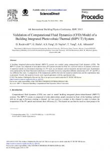
This final velocity prediction program gathers the experimental hydrodynamic and .... ___ 19. Figure 14: Code for importing the model geometry into FS Flow.
Development and Validation of a Computational Fluid Dynamics Hydrodynamic Model of the Stewart 34 for Velocity Prediction Program Applications
Jean-Baptiste Roger Guillaume SOUPPEZ 9997513
Supervisor:
Dr. Stuart E. NORRIS
Master of Engineering Studies in Yacht Engineering MechEng 775 – Yacht Engineering Project Department of Mechanical Engineering The University of Auckland November 2014
Development and Validation of a CFD Hydrodynamic Model of the Stewart 34 for VPP Applications
Abstract
The prediction of the hydrodynamic behaviour of sailing yachts is a key component of modern yacht design, particularly to assess the theoretical performance of a design through a velocity prediction program. The increasing computational power now offers an alternative to towing tank testing: computational fluid dynamics. The work conducted on the development and validation of a computational fluid dynamics hydrodynamic model of the Stewart 34 sailing yacht for velocity prediction program applications is presented in this report. An empirical resistance model has initially been developed based on the Delft Systematic Yacht Hull Series. The method has been described and its limitations highlighted, the main ones being the resistance prediction in semi-displacement mode and the side force prediction at high leeway angle. The method is however reliable for common designs in displacement mode and is particularly efficient since only a few design inputs are required. In a second time, the use of the Rankine source panel code FS-Flow led to a computational fluid dynamics hydrodynamic model of the Stewart 34, validated against an experimental benchmark, as done for the empirical resistance calculations. Instabilities in the panel code at high Froude numbers resulted in a loss of accuracy. Furthermore, the panel code did not prove suitable at high leeway angles. FS-Flow appears to have some limitations when handling the hydrodynamic model of sailing yachts; its intended use primarily being the comparison of ship designs. A total of three velocity prediction programs have been developed. An empirical 4 degrees of freedom one enabled to ascertain the test matrix for the Stewart 34. A second 4 degrees of freedom one was realised with WinDesign to provide a reference and comparison with the final 6 degrees of one done using FS-Equilibrium. This final velocity prediction program gathers the experimental hydrodynamic and aerodynamic models and was validated against available upwind full scale data to ensure its reliability. A complete performance prediction for the Stewart 34 was therefore achieved based on experimental data, mostly focussing on the hydrodynamic model ascertained using both empirical and computational fluid dynamics methods, thus meeting the objectives set for this project. Finally, areas of further improvement and future work have been recommended.
Jean-Baptiste R. G. SOUPPEZ
III
Development and Validation of a CFD Hydrodynamic Model of the Stewart 34 for VPP Applications
Acknowledgements
The author would like to thank the following individuals for their much appreciated contribution to this project.
Dr. Stuart Norris, supervisor of the project, for his invaluable help and support throughout the duration of the project.
David Le Pelley, owner of Pride, for his help and information inherent to the Stewart 34.
Dr. Heikki Hansen, and the FutureShip company, for providing the CFD and VPP software essential to the project, and his much appreciated advice regarding the velocity prediction program.
George Backhus, author of “Stewart 34 Yachting: the first 50 years”, for providing a copy of his book and the original plans of the Stewart 34.
Marco Boscarino and Lan Yu, for sharing their experimental aerodynamic data, used for the realisation of the VPP.
IV
Jean-Baptiste R. G. SOUPPEZ
Development and Validation of a CFD Hydrodynamic Model of the Stewart 34 for VPP Applications
Table of Contents
ABSTRACT
III
ACKNOWLEDGEMENTS
IV
TABLE OF CONTENTS
V
LIST OF FIGURES
VIII
LIST OF TABLES
IX
LIST OF SYMBOLS
X
LIST OF GREEK SYMBOLS
XI
LIST OF ACRONYMS
XI
CHAPTER 1: INTRODUCTION
1
1.1 PROJECT OUTLINE 1.2 STEWART 34
1 2
CHAPTER 2: PREVIOUS WORK
5
CHAPTER 3: DSYHS EMPIRICAL HYDRODYNAMIC MODEL
7
3.1 RESISTANCE MODELS 3.1.1 FROUDE MODEL 3.1.2 FRICTION COEFFICIENT 3.1.3 ITTC 78 MODEL 3.1.4 PROHASKA METHOD 3.2 VALIDATION 3.2.1 DELFT REPRESENTATIVE HULL FORM 3.2.2 METHOD VALIDATION 3.2.3 UNCERTAINTIES 3.2.4 CONCLUSIONS 3.3 APPLICATION TO THE STEWART 34 3.3.1 DSYHS RANGE OF PARAMETERS 3.3.2 APPLICATION OF THE DSYHS TO THE STEWART 34 3.3.3 ADDITIONAL CONSIDERATIONS 3.4 DSYHS: PRESENT AND FUTURE WORK 3.5 CONCLUSIONS CHAPTER 4: CFD ANALYSIS AND VALIDATION 4.1 RANKINE SOURCE PANEL CODE 4.1.1 FAST SOLVING 4.1.2 DISADVANTAGES OF PANEL CODE 4.1.3 FS-FLOW 4.2 FS-FLOW: SETUP AND USE 4.2.1 CONVERTING GEOMETRY 4.2.2 IMPORTING GEOMETRY 4.2.3 MESHING 4.2.4 SET UP 4.2.5 RESULTS
Jean-Baptiste R. G. SOUPPEZ
7 7 8 8 8 9 9 10 13 14 15 15 15 16 17 18 19 19 19 20 20 21 21 21 22 23 24 V
Development and Validation of a CFD Hydrodynamic Model of the Stewart 34 for VPP Applications
4.3 VERIFICATION AND VALIDATION: SYSSER 62 4.3.1 DOMAIN SIZE 4.3.2 KELVIN WAVE PATTERN 4.3.3 MESH DENSITY 4.3.4 CONVERGENCE STUDY 4.3.5 ERROR ESTIMATION 4.3.6 SOLVING TIME 4.3.7 RESULTS 4.3.8 CONCLUSIONS 4.4 APPLICATION TO THE STEWART 34 4.4.1 TEST MATRIX 4.4.2 ANALYSIS OF THE STEWART 34 4.4.3 CONCLUSIONS 4.5 CONCLUSIONS
24 25 25 26 27 27 29 30 32 33 33 33 34 34
CHAPTER 5: VELOCITY PREDICTION PROGRAM
36
5.1 SIX DEGREES OF FREEDOM 5.1.1 FORCES 5.1.2 MOMENTS 5.1.3 VPP AND DEGREES OF FREEDOM 5.2 EMPIRICAL 4 DEGREES OF FREEDOM VPP 5.2.1 PRINCIPLE 5.2.2 RESULTS 5.2.3 CONCLUSIONS 5.3 WINDESIGN 5.3.1 PRINCIPLE 5.3.2 RESULTS 5.3.3 CONCLUSIONS 5.4 FS-EQUILIBRIUM: SETUP 5.4.1 PRINCIPLE 5.4.2 COORDINATE SYSTEM 5.4.3 MODIFICATION OF EXPERIMENTAL DATA 5.4.4 EXPERIMENTAL HYDRODYNAMIC MODULE 5.4.5 BUOYANT VOLUME MODULE 5.5 APPLICATION TO THE STEWART 34 5.5.1 VPP RESULTS 5.5.2 IMPACT OF THE RUDDER 5.5.3 IMPACT OF PITCH AND HEAVE 5.5.4 VALIDATION 5.5.5 CONCLUSIONS 5.5 CONCLUSIONS
36 37 37 37 38 38 38 39 39 39 40 41 41 41 41 42 43 43 43 44 45 45 45 46 46
CHAPTER 6: CONCLUSIONS AND RECOMMENDATIONS
48
6.1 CONCLUSIONS 6.1.1 DELFT SYSTEMATIC YACHT HULL SERIES 6.1.2 COMPUTATIONAL FLUID DYNAMICS: FS-FLOW 6.1.3 VELOCITY PREDICTION PROGRAM: FS-EQUILIBRIUM 6.1.4 CONCLUSIONS 6.2 RECOMMENDATIONS FOR FUTURE WORK
48 48 48 49 49 50
REFERENCES
52
APPENDICES
58
VI
Jean-Baptiste R. G. SOUPPEZ
Development and Validation of a CFD Hydrodynamic Model of the Stewart 34 for VPP Applications
A. DSYHS CALCULATION METHOD A.1 UPRIGHT: BARE HULL A.2 UPRIGHT: APPENDAGES A.3 HEELED: BARE HULL A.4 EXTENDED KEEL METHOD A.5 HEELED: APPENDAGES A.6 YAWED: APPENDAGES B. WAVE PATTERNS C. DSYHS EXAMPLES OF HIGH FROUDE NUMBER RESISTANCE PREDICTION D. VALIDATION OF THE SYSSER 62 HYDRODYNAMIC MODEL D.1 10° HEEL D.2 20° HEEL D.3 30° HEEL E. TABLE OF OFFSETS OF THE STEWART 34 E.1 ORIGINAL IMPERIAL MEASUREMENTS E.2 METRIC CONVERSION F. THREE DIMENSIONAL LOFTING G. EMPIRICAL 4 DEGREES OF FREEDOM VPP G.1 HYDRODYNAMIC MODEL G.2 VELOCITY TRIANGLES G.3 AERODYNAMIC MODEL G.4 STABILITY G.5 DEPOWERING G.6 RUDDER ANGLE H. HYDRODYNAMIC MODEL OF THE STEWART 34 H.1 UPRIGHT H.2 7.5° HEEL H.3 15° HEEL H.4 22.5° HEEL H.5 28° HEEL H.6 35° HEEL I. TRANSVERSE STABILITY ASSESSMENT I.1 SMALL ANGLE STABILITY I.2 INCLINING EXPERIMENT I.3 LARGE ANGLE STABILITY I.4 FURTHER CONSIDERATIONS I.5 CONCLUSIONS J COMPARISON OF FS-EQUILIBRIUM AND WINDESIGN K. VELOCITY PREDICTION PROGRAM RESULTS FOR THE STEWART 34 K.1 BOAT SPEED (M/S) K.2 BOAT SPEED (KTS) K.3 HEEL ANGLE K.4 LEEWAY ANGLE K.5 RUDDER ANGLE K.6 PITCH ANGLE
Jean-Baptiste R. G. SOUPPEZ
58 58 59 60 61 62 62 64 65 66 66 66 67 68 68 68 69 72 72 72 72 74 75 75 78 78 79 80 81 82 83 84 84 85 88 89 90 91 94 94 95 96 97 98 99
VII
Development and Validation of a CFD Hydrodynamic Model of the Stewart 34 for VPP Applications
List of Figures
Figure Figure Figure Figure Figure Figure Figure Figure Figure Figure Figure Figure Figure Figure Figure Figure Figure Figure Figure Figure Figure Figure Figure Figure Figure Figure Figure Figure Figure Figure Figure Figure Figure Figure Figure Figure Figure Figure Figure Figure Figure Figure Figure Figure Figure Figure Figure Figure Figure Figure
VIII
1: Stewart 34 sailplan [85]. ______________________________________________________ 2 2: Stewart 34 linesplan [84]. _____________________________________________________ 3 3: Gray Dixon Rudder [2]. ________________________________________________________ 4 4: Original linesplan of the Stewart 34, drawn by Robert Stewart in 1959 [84]. ___________ 9 5: Sysser 62 linesplan [18]. ______________________________________________________ 10 6: Sysser 3 linesplan [18]. _______________________________________________________ 10 7: Upright total hull resistance, Sysser 62. _________________________________________ 11 8: Total upright resistance of the Sysser 3 and Sysser 62. ____________________________ 11 9: DSYHS and experimental data [18] comparison at 10° of heel. ______________________ 12 10: Experimental appendages resistance of the Sysser 62 [18]. ________________________ 14 11: Stewart 34 upright resistance components. _____________________________________ 15 12: Stewart 34 final upright resistance components. ________________________________ 17 13: Design tool usage in the America’s Cup from 1995 to 2010. Data edited from [91]. ___ 19 14: Code for importing the model geometry into FS Flow. ____________________________ 21 15: Sysser 62 meshing (exaggerated for clarity) realised in FS-Flow. ___________________ 22 16: Illustration of the keel wake for the Sysser 62.__________________________________ 23 17: Typical FS-Flow simulation. __________________________________________________ 24 18: Impact of the domain size on the resistance (𝛥𝑥=0.05).___________________________ 25 19: Kelvin wave pattern check. __________________________________________________ 26 20: Impact of the mesh density on the resistance. __________________________________ 26 21: Convergence study at Fn = 0.25. ______________________________________________ 27 22: Convergence study at Fn = 0.45. ______________________________________________ 27 23: Variation of the solving time with Froude number. ______________________________ 29 24: Variation of the solving time with the number of elements at Fn = 0.30. ____________ 30 25: Variation of solving time with error at Fn = 0.30. _______________________________ 30 26: Bare hull upright resistance of the Sysser 62. ___________________________________ 31 27: DSYHS, experimental data and CFD comparison at 10° of heel. ____________________ 31 28: Typical example of FS-Flow results for the hydrodynamic model of the Stewart 34.___ 34 29: Six degrees of freedom illustration, edited from [51]. ___________________________ 36 30: Stewart 34 VPP using WinDesign. ______________________________________________ 40 31: Typical example of modified resistance values. _________________________________ 42 32: Typical example of modified side force values. _________________________________ 42 33: Fs-Equilibrium VPP, boat speed (knots). ________________________________________ 44 34: Impact of pitch and heave on boat speed. ______________________________________ 45 35: Experimental [10] and VPP comparison. ________________________________________ 46 36: Extended keel method illustration, edited from [60]. ____________________________ 61 37: Wave pattern at a Froude number of 0.40. _____________________________________ 64 38: Wave pattern at a Froude number of 0.50. _____________________________________ 64 39: Wave pattern at a Froude number of 0.60. _____________________________________ 64 40: Case of over-predicted resistance by the DSYHS (unknown model), from [54]. ________ 65 41: Case of under-predicted resistance by the DSYHS (model 329), from [56]. ___________ 65 42: DSYHS, experimental data and CFD comparison at 10° of heel. ____________________ 66 43: DSYHS, experimental data and CFD comparison at 20° of heel. ____________________ 66 44: DSYHS, experimental data and CFD comparison at 30° of heel. ____________________ 67 45: Half cylinder, starting point of the 3D lofting. __________________________________ 69 46: Surface net matching the tables of offsets grid. _________________________________ 69 47: Net of the 3D lofted Stewart 34 ______________________________________________ 70 48: Additional waterline added to the model of the Stewart 34. ______________________ 70 49: Final model of the Stewart 34. _______________________________________________ 71 50: Stewart 34 hydrodynamic model: FS-Flow and DSYHS comparison, 0° Heel. __________ 78
Jean-Baptiste R. G. SOUPPEZ
Development and Validation of a CFD Hydrodynamic Model of the Stewart 34 for VPP Applications
Figure Figure Figure Figure Figure Figure Figure Figure Figure Figure Figure Figure Figure Figure Figure Figure Figure Figure Figure Figure Figure
51: Stewart 34 hydrodynamic model: FS-Flow and DSYHS comparison, 7.5° Heel. ________ 79 52: Stewart 34 hydrodynamic model: FS-Flow and DSYHS comparison, 15° Heel._________ 80 53: Stewart 34 hydrodynamic model: FS-Flow and DSYHS comparison, 22.5° Heel. _______ 81 54: Stewart 34 hydrodynamic model: FS-Flow and DSYHS comparison, 28° Heel. _________ 82 55: Stewart 34 hydrodynamic model: FS-Flow and DSYHS comparison, 35° Heel. _________ 83 56: Transverse stability at small heel angles. ______________________________________ 84 57: Model scale inclining experiment illustrating a typical setup. _____________________ 85 58: Pendulum setup for the inclining experiment of the Stewart 34, illustration from [79]. 87 59: Gz curve of the Stewart 34 ascertained using Hydromax [8]. ______________________ 88 60: Midship trough, picture from [6]. _____________________________________________ 89 61: Speed difference (kts) between FS-Equilibrium and WinDesign. ___________________ 91 62: Heel difference (°) between FS-Equilibrium and WinDesign. ______________________ 91 63: Leeway difference (°) between FS-Equilibrium and WinDesign. ____________________ 92 64: Reef difference between FS-Equilibrium and WinDesign. _________________________ 92 65: Flat difference between FS-Equilibrium and WinDesign. __________________________ 93 66: Stewart 34 FS-Equilibrium VPP: boat speed (m/s). ______________________________ 94 67: Stewart 34 FS-Equilibrium VPP: boat speed (kts). _______________________________ 95 68: Stewart 34 FS-Equilibrium VPP: heel angle(°). __________________________________ 96 69: Stewart 34 FS-Equilibrium VPP: leeway angle (°). _______________________________ 97 70: Stewart 34 FS-Equilibrium VPP: rudder angle (°). _______________________________ 98 71: Stewart 34 FS-Equilibrium VPP: pitch angle (°). _________________________________ 99
List of Tables
Table Table Table Table Table Table Table Table Table Table Table Table Table Table Table Table Table
1: Hydrostatics of the Stewart 34 Pride. ____________________________________________ 3 2: DSYHS range of parameters [58]. _______________________________________________ 15 3: Free surface intersections. ____________________________________________________ 22 4: Richardson extrapolation and error estimation at various Froude numbers. ___________ 29 5: Maximum values ascertained using the empirical VPP. _____________________________ 38 6: DSYHS upright hull residuary resistance regression coefficients [56]. ________________ 58 7: New hull residuary resistance coefficients [54]. __________________________________ 59 8: DSYHS upright appendages residuary resistance regression coefficients [58]. __________ 60 9: DSYHS heeled wetted surface area regression coefficients [56]. _____________________ 60 10: DSYHS 20° of heel hull delta residuary resistance regression coefficients [56]. _______ 61 11: DSYHS heeled appendages delta residuary resistance regression coefficients [58]. ____ 62 12: DSYHS effective draft regression coefficients [56]. _______________________________ 62 13: Original table of offsets of the Stewart 34 [84]. _________________________________ 68 14: Table of offsets of the Stewart 34, converted into metric units from [84]. __________ 68 15: Offshore Racing Congress sail coefficients [69]. _________________________________ 72 16: Windage coefficients, as defined in [93]. _______________________________________ 74 17: Righting lever for the Stewart 34. _____________________________________________ 88
Jean-Baptiste R. G. SOUPPEZ
IX
Development and Validation of a CFD Hydrodynamic Model of the Stewart 34 for VPP Applications
List of Symbols
1+𝑘 𝐴𝑓 𝐴𝑙𝑎𝑡 𝐴𝑚𝑎𝑥 𝐴𝑝 𝐴𝑅 𝐴𝑅𝑒 𝐴𝑅𝑔 𝐴𝑤 𝑏 𝐵𝐴𝐷 ̅̅̅̅̅ 𝐵𝑀 𝐵𝑂𝐴 𝐵𝑤𝑙 𝑐̅ 𝐶𝑎 𝐶𝐷𝑖 𝐶𝐷𝑝 𝐶𝐷𝑤 𝐶𝐸 𝐶𝑓 𝐶𝐿 𝐶𝐿𝑅 𝐶𝑚 𝐶𝑝 𝐶𝑃𝑃 𝐶𝑟 𝐶𝑡 𝐶𝑡 𝐶𝑣 𝐶𝑤 𝑓 𝑓 𝐸 𝐸𝑀𝐻 𝐹𝐴 𝐹ℎ 𝐹𝑛 𝐹𝑃𝑃 𝑔 ̅̅̅̅̅ 𝐺𝐺′ ̅̅̅̅̅ 𝐺𝑀 ̅𝐺𝑧 ̅̅̅ 𝐻𝐴 𝐻𝑀 𝐼 𝐼𝑡 𝐼𝑥𝑥 𝐽
X
Form factor Frontal area Lateral area Maximum section area Projected area Aspect ratio Effective aspect ratio Geometric aspect ratio Waterplane area Span Boom above deck Metacentric radius Beam overall Waterline beam Mean chord length Roughness coefficient Induced drag coefficient Parasitic drag coefficient Windage drag coefficient Centre of effort ITTC 57 Frictional coefficient Lift coefficient Centre of lateral resistance Midship area coefficient Prismatic coefficient Propeller drag coefficient Root chord length Total resistance coefficient Tip chord length Viscous coefficient Wave coefficient Froude’s friction coefficient Flat Mainsail foot Mast height Freeboard Side force Froude number Forward perpendicular Acceleration due to gravity Centre of gravity correction Metacentric height Righting lever Heeling arm Heeling moment Fore triangle height Second moment of area of a tank Second moment of area of the waterplane Fore triangle base
𝐾𝑆𝐹 𝐿𝐶𝐵 𝐿𝐶𝐵𝑓𝑝𝑝 𝐿𝐶𝐹 𝐿𝐶𝐹𝑓𝑝𝑝 𝐿𝑂𝐴 𝐿𝑃 𝐿𝑝𝑝 𝐿𝑤𝑙 𝑀𝐷 𝑝 𝑃 𝑆𝐴𝐶 𝑆𝑐 𝑆𝑐𝜑 𝑆𝐹 𝑆𝐿 𝑆𝑆𝐹 𝑟 𝑅𝑎 𝑅𝑓 𝑅𝑖 𝑅𝑛 𝑅𝑝 𝑅𝑟 𝑅𝑡 𝑅𝑡𝜑 𝑅𝑣 𝑅𝑣𝜑 𝑅𝑤 𝑅𝑤𝜑 𝑇 𝑡/𝑐 𝑇𝑐 𝑇𝑒 𝑇𝑟 𝑉 𝑉𝑎 𝑉𝐶𝐵 𝑉𝐶𝐺 𝑉𝑡 𝑍𝑐𝑏𝑎𝑝𝑝
Keel side force Longitudinal centre of buoyancy aft of amidships Longitudinal centre of buoyancy from the forward perpendicular Longitudinal centre of flotation aft of amidships Longitudinal centre of flotation from the forward perpendicular Length over all Luff perpendicular Length between perpendiculars Waterline length Mast diameter Power Mainsail luff Sectional area coefficient Upright canoe body wetted surface area Heeled canoe body wetted surface area Side force Spinnaker luff Sail side force Reef Roughness resistance Frictional resistance Induced resistance Reynolds number Propeller resistance Residuary resistance Total resistance Heeled total resistance Viscous resistance Heeled viscous resistance Wave resistance Heeled wave resistance Overall draft Thickness/chord ratio Canoe body draft Effective draft Taper ratio Velocity Apparent wind speed Vertical centre of buoyancy Vertical centre of gravity True wind speed Vertical centre of buoyancy of an appendage
Jean-Baptiste R. G. SOUPPEZ
Development and Validation of a CFD Hydrodynamic Model of the Stewart 34 for VPP Applications
List of Greek Symbols
𝛼 𝛽 𝛽𝑎 𝛽𝑡 𝛥 𝛥𝑥 𝛥𝑅𝑟 𝛥𝑅𝑟𝜑 ∇app ∇c 𝜃 𝜆 𝜇 𝜌 𝜑
Rudder angle of attack Yaw angle Apparent wind angle True wind angle Displacement Mesh grid spacing Delta in residuary resistance Delta in heeled residuary resistance Appendages displaced volume Canoe body displaced volume Pitch angle Leeway angle Viscosity Density Heel angle
List of Acronyms
AWA AWS CDF DSYHS FSE GCI IGES ITTC NURBS ORC RANSE Sysser TFWT TWA TWS VCG VMG VPP YRU
Apparent Wind Angle Apparent Wind Speed Computational Fluid Dynamics Delft Systematic Yacht Hull Series Free Surface Effect Grid Convergence Index Initial Graphics Exchange Specification International Towing Tank Conference Non-Uniform Radial B-Splines Offshore Racing Congress Reynolds Averaged Navier-Stokes Equations Systematic Serie Twister Flow Wind Tunnel True Wind Angle True Wind Speed Vertical Centre of Gravity Velocity Made Good Velocity Prediction Program Yacht Research Unit
Jean-Baptiste R. G. SOUPPEZ
XI
Development and Validation of a CFD Hydrodynamic Model of the Stewart 34 for VPP Applications
Chapter 1: Introduction
1.1 Project Outline The ability to predict the velocity and behaviour of a boat enables to refine the design in a first place, and then to optimise the performances on the water. This is the crucial role played by Velocity Prediction Programs (VPP) in modern yacht design; hence the need for a reliable hydrodynamic model. Previously, the evaluation of the hydrodynamic resistance and side force was done using either empirical calculations, or towing tank tests. The Delft Systematic Yacht Hull Series (DSYHS) offers a good starting point for common hull forms; however, this empirical method does not suit every boat, and the accuracy is questionable. A much more accurate option is towing tank testing; unfortunately this process is time consuming, very expensive, and requires the appropriate facilities, which are not available in New Zealand. With the evolution of technology rose a new method that would fill the gap between the inaccurate and inexpensive empirical methods, and the more reliable but expensive and time consuming towing tank testing: Computational Fluid Dynamics (CFD). In theory, CFD enables to achieve a reliable hydrodynamic model, faster and at a lesser cost than towing tank testing. A panel code approach has been adopted in this instance for its lesser solving time compared to a Reynolds-Averaged Navier-Stokes solver. The project has been developed with a particular emphasis on the validation of the methods proposed. As a result, towing tank data have been used as a benchmark to validate the DSYHS calculations as well as the panel code, in order to have confidence in the accuracy of the final hydrodynamic model. This is mainly motivated by the absence of publications and information related to the use of the panel code FS-Flow. This project will provide an insight into the use and reliability of CFD-based hydrodynamic resistance and side force for VPP applications, focussing on a given boat: the Stewart 34. The vessel has been chosen as it is used as a test boat by the Yacht Research Unit (YRU) and so experimental sail data is available [99, 12]. However, the absence of hydrodynamic model for the boat prevents the creation of an accurate VPP, hence the primary objective of this project, which is a continuation of the work undertaken by Sammour [79]. First of all, the DSYHS and the CFD analysis will be validated against the experimental data of the Sysser 62, elected as a benchmark thanks to its resemblance with the Stewart 34. An empirical and a CFD hydrodynamic model will then be developed for the Stewart 34. Finally, the experimental sail data will be used to realise a 6 degrees of freedom VPP. The project being focused on the Stewart 34, the vessel will be presented in the following section, essentially based on the publication by George Backhus on the history of the Stewart 34 Class [2].
Jean-Baptiste R. G. SOUPPEZ
1
Development and Validation of a CFD Hydrodynamic Model of the Stewart 34 for VPP Applications
1.2 Stewart 34 Designed by Robert Stewart in 1959, the Stewart 34 is undeniably a major part of New Zealand maritime history. The 34 feet vessel seduced by both its speed on the water and the large accommodation volume, making it a competitive racer as well as a comfortable family cruiser. The design slightly evolved over the years, the most significant evolution being the change from wood to fibreglass. Nonetheless, accurately calculated ballast weights enable both types of boats to race together, leading to one of the largest one-design fleet in New Zealand [2]. Digitalised copies of the original sailplan and linesplan, conserved at the New Zealand Maritime Museum in Auckland, are respectively presented in Figure 1 and Figure 2.
Figure 1: Stewart 34 sailplan [85].
2
Jean-Baptiste R. G. SOUPPEZ
Development and Validation of a CFD Hydrodynamic Model of the Stewart 34 for VPP Applications
Figure 2: Stewart 34 linesplan [84].
The project will be based on a particular vessel, Pride, weighed at 5100 kg. The hydrostatics of the vessel for this particular displacement are listed in Table 1 and will be the basis of the empirical resistance model presented in Chapter 3. Stewart 34 Hydrostatics Length over all - LOA (m) Waterline length - Lwl (m) Beam over all - BOA (m) Waterline beam - Bwl (m) Canoe body draft - Tc (m) Total draft - T (m) Total displacement - Δ (t) 3 Canoe body volume - ∇c (m ) Wetted surface area - Sc (m²) Waterplane area - Aw (m²) LCB from FPP - LCBfpp (m) LCF from FPP - LCFfpp (m) Prismatic coefficient - Cp Midship coefficient - Cm
10.44 9.45 3.10 2.71 0.53 1.67 5.10 4.67 19.20 17.37 4.89 5.18 0.54 0.65
Table 1: Hydrostatics of the Stewart 34 Pride.
Furthermore, it is to be noted that the vessel considered does not feature the skeg-rudder illustrated on the linesplan (Figure 2) but the Gray Dixon rudder: a later design improvement of the Stewart 34 [2], shown in Figure 3. As a result, the hydrodynamic model will be developed for this rudder configuration.
Jean-Baptiste R. G. SOUPPEZ
3
Development and Validation of a CFD Hydrodynamic Model of the Stewart 34 for VPP Applications
Figure 3: Gray Dixon Rudder [2].
Having introduced the Stewart 34, the background and previous work will be presented in order to set the context and motivations behind the topic tackled in this project.
4
Jean-Baptiste R. G. SOUPPEZ
Development and Validation of a CFD Hydrodynamic Model of the Stewart 34 for VPP Applications
Chapter 2: Previous work
For the past few years, the Yacht Research Unit (YRU) has undertaken experimental work on the sails of the Stewart 34, at both model and full scale. Aerodynamic coefficients have been ascertained for upwind [99] and downwind [12] sails, with particular emphasis on depowering, clearly demonstrating the intended use for VPP purposes. This calls for a full hydrodynamic model of the yacht in order to obtain the resistance and side force to balance the aerodynamic drive and side force, and therefore predict the performances of the Stewart 34. The most notable work in this area was performed in 2012 by Sammour [79] that developed a CFD hydrodynamic model based on the panel code FS-Flow, leading to an upwind VPP of the Stewart 34. However, some limitations and areas of further improvement have been identified, and are detailed hereafter: 1. The use of the Delft Systematic Yacht Hull Series (DSYHS) as an empirical resistance model was not thoroughly defined, and its application and limitations were not clearly established. The method will therefore be described and validated against an experimental benchmark in order to identify possible limitations before being applied to the Stewart 34. All aspects of the DSYHS have been gathered and presented by Keuning and Sonnenber [56] in 1998. However, updates parts of the methods have been published in more recent years, mainly regarding the appendages [53] and bare hull [54] calculations. 2. The hydrodynamic model did not consider the rudder, which is a non-negligible component both in terms of resistance and side force generated. This also raises the issue of the keel wake modelling with a panel code. The original plans of the Gray Dixon rudder have been obtained [2] and checked against to measurements realised on the boat, thus enabling to model and include the rudder as part of the CFD simulations and resulting hydrodynamic model of the Stewart 34. 3. No validation of the panel code was conducted. The analysis is performed with FS-Flow [24], a panel code that is not widely used, and for which no publication is available (with the exception of the user manual [26]). The panel code was developed for the purpose of comparing ship designs, and very little is known about its potential ability to model sailing yachts. A careful validation against experimental results is therefore required to ensure the reliability of the hydrodynamic model of the Stewart 34. The project will also aim at providing details regarding the general use of the panel code to facilitate future use. 4. The range of parameters previously considered for the CFD simulations appears quite extensive and not relevant to the sailing behaviour of the yacht. On the one hand, the range of leeway tested (from -2° to 10°) extends beyond the sailing range of leeway angles, resulting in unnecessary computations. On the other hand, the heel angles have been tested up to 20° only when the VPP ascertains heel angles greater than 30°. There is therefore a large source of uncertainty introduced, and an extended range of heel angles should be tested for. To remedy this issue, and empirical VPP will be developed at an early stage of the project to establish the relevant test matrix.
Jean-Baptiste R. G. SOUPPEZ
5
Development and Validation of a CFD Hydrodynamic Model of the Stewart 34 for VPP Applications
5. The stability of the Stewart 34 was assessed thanks to an inclining experiment [79]. However, the rise in centre of gravity due to the presence of the inclining weights on deck during the experiment was not accounted for. As a result, the centre of gravity and inherent stability curve ascertained are not representative of the actual boat. The stability calculations will therefore be performed from the raw data of the experiment in order to establish the location of the vertical centre of gravity of the Stewart 34, and then used to develop the righting lever curve. 6. Due to the absence of data for downwind sails, only the upwind VPP has been assessed by Yu [99]. The experimental aerodynamic model of the Stewart 34 for downwind sails has recently been developed [12] based on model scale testing performed at the Twisted Flow Wind Tunnel. Aerodynamic data including depowering is therefore available. Furthermore, despite the experimental CFD hydrodynamic model of the Stewart 34 previously developed, the VPP appears to be based on the empirical resistance modules of the VPP [99]. Inputting the actual CFD data generated will be tackled in this instance, leading to a complete experimental velocity prediction for the Stewart 34. Particular attention will be paid to improve those various aspects in order to provide a thoroughly defined empirical model based on the DSYHS as well as a validated CFD model. The refined stability of the vessel and the latest downwind wind tunnel data will then be used to ascertain an accurate 6 degrees of freedom VPP of the Stewart 34.
6
Jean-Baptiste R. G. SOUPPEZ
Development and Validation of a CFD Hydrodynamic Model of the Stewart 34 for VPP Applications
Chapter 3: DSYHS Empirical Hydrodynamic Model
The Delft Systematic Yacht Hull Series (DSYHS) gathers over 70 hulls towing tank tested, the results for the first 62 of them being available online [18]. From the results, regression formulae have been developed to predict the resistance of a given vessel based on its principal dimensions and design ratios. This empirical method is only valid provided the design fits within the range of parameters considered by the DSYHS; but the idea that the resistance can be estimate based on design parameters only, as opposed to a defined hull shape, enables to consider the resistance at a very early stage of the design, prior to drawing the actual hull shape. Despite the debatable accuracy of the method, the DSYHS stands nowadays as a perfectly valid resistance prediction method, even if a refined resistance prediction based on either towing tank testing or CFD would be advised for the final design, especially when speed is a critical factor. The resistance model and inherent calculations will be presented for the hull and appendages, in upright and heeled and yawed cases. The validity of the DSHYS prediction will be assessed against a vessel with known towing tank results before being applied to the Stewart 34.
3.1 Resistance Models The resistance of yachts can be broken down according to two resistance models: the original Froude model presented by William Froude in 1872 [21, 22] and the more recent model adopted at the 1978 International Towing Tank Conference (ITTC) [41, 42].
3.1.1 Froude Model The resistance model proposed by William Froude strips down the resistance into two main components: frictional resistance 𝑅𝑓 and residuary resistance 𝑅𝑟 [21, 42]. Froude considers the frictional resistance to be equal to the resistance of a flat plate having the same wetted area as the boat, the other components of resistance being comprised in the residuary resistance; mathematically the total resistance 𝑅𝑡 is therefore given by: 𝑅𝑡 = 𝑅𝑓 + 𝑅𝑟
Equation 1
After testing a wide range of flat plates, Froude derived a formula to estimate the frictional resistance [4, 42] based on the wetted area 𝑆𝑐 and the velocity 𝑉: 𝑅𝑓 = 𝑓 × 𝑆𝑐 × 𝑉 1.825
Equation 2
Where 𝑓 is the friction coefficient, defined as: 𝑓=
1 0.258 × ((0.1392 + ) × 𝜌𝑤𝑎𝑡𝑒𝑟 ) 1000 2.68 + 𝐿𝑤𝑙
Equation 3
Froude’s resistance model is still valid nowadays; in fact, it is the resistance model adopted by the DSYHS for reasons explained in Section 3.1.4. However, the expression for the friction coefficient has been refined over the years.
Jean-Baptiste R. G. SOUPPEZ
7
Development and Validation of a CFD Hydrodynamic Model of the Stewart 34 for VPP Applications
3.1.2 Friction Coefficient The introduction of the Reynolds number 𝑅𝑛 in 1883 [76] led to new definitions of the friction coefficient [4] eventually leading to the ITTC 1957 formula [32]: 𝐶𝑓 =
0.075 (log10 𝑅𝑛 − 2)2
Equation 4
From this new friction coefficient, the ITTC developed an alternative resistance model.
3.1.3 ITTC 78 Model The main difference in the ITTC 78 resistance model is the introduction of a form factor 1 + 𝑘 which multiplied by the frictional resistance gives the 3 dimensional viscous resistance 𝑅𝑣 [41]: 𝑅𝑣 = (1 + 𝑘) × 𝑅𝑓
Equation 5
Where 𝑅𝑓 is based on the ITTC 57 friction coefficient: 𝑅𝑓 =
1 × 𝜌 × 𝑆𝑐 × 𝑉² × 𝐶𝑓 2
Equation 6
The form factor represents the effect of the hull shape on the friction resistance, hence its definition of a 3D viscous resistance as opposed to the 2D flat plates considered by Froude. The remaining components of the resistance are gathered in the wave resistance 𝑅𝑤, giving the ITTC resistance model as: 𝑅𝑡 = 𝑅𝑣 + 𝑅𝑤
Equation 7
The value of the form factor for a given boat is ascertained using the Prohaska method.
3.1.4 Prohaska Method The Prohaska method [72] enables to assess the value of the form factor based on towing tank testing. Prohaska makes similar assumptions as the ITTC 78 (stated in equations 5 and 7), which in terms of coefficients gives: 𝐶𝑣 = (1 + 𝑘) × 𝐶𝑓
Equation 8
𝐶𝑡 = 𝐶𝑣 + 𝐶𝑤
Equation 9
According to Baba [1] at low speeds, the wave coefficient 𝐶𝑤 can be calculated by: 𝐶𝑤 = 𝑎 × 𝐹𝑛4
Equation 10
𝐶𝑡 = 𝑎 × 𝐹𝑛4 + (1 + 𝑘) × 𝐶𝑓
Equation 11
𝐶𝑡 𝐹𝑛4 =𝑎× + (1 + 𝑘) 𝐶𝑓 𝐶𝑓
Equation 12
Combining equations 8, 9 and 10:
Dividing by 𝐶𝑓:
Therefore giving the equation of a straight line of the form: 𝑦 =𝑚×𝑥+𝑐
8
Equation 13
Jean-Baptiste R. G. SOUPPEZ
Development and Validation of a CFD Hydrodynamic Model of the Stewart 34 for VPP Applications
Where: 𝑦=
𝐶𝑡 𝐶𝑓
𝑚=𝑎
𝑥=
𝐹𝑛4 𝐶𝑓
𝑐 =1+𝑘
Plotting 𝐹𝑛4 /𝐶𝑓 against 𝐶𝑡/𝐶𝑓, the y-intercept of the best fit line will give the form factor 1 + 𝑘. This is known as a Prohaska Plot, only valid for slow speeds where the wave resistance is negligible and the viscous drag is the dominant component of the resistance. As a result, values of 𝐹𝑛4 /𝐶𝑓 greater than 4 should not be considered [4]. The Prohaska method requires experimental data to establish the form factor. The absence of numerical method to calculate 1 + 𝑘, coupled with the will to offer an alternative method to towing tank testing led the DSYHS not to consider the form factor [59] effectively basing their resistance breakdown on Froude’s model. The DSYHS calculation process and inherent hydrodynamic model is thoroughly presented and detailed in Appendix A, and will be used for the purpose of the validation of the method.
3.2 Validation In order to validate the DSYHS method, the resistance prediction will be compared to actual towing tank data for a known vessel from the DSYHS database [18]. For the validation to be more relevant, a suitable hull must be selected among the 62 available.
3.2.1 Delft Representative Hull Form The selected DSYHS hull must cover an appropriate range of Froude numbers and a wide range of experimental results. In addition, a hull similar to the Steward 34 in terms of design parameters must be chosen. Finally, the hull shape must resemble the Stewart 34, with similar design features. Initially, series with limited experimental data have been eliminated. A statistical analysis of the difference in design parameters has been conducted on the remaining series. Finally, the representative hull has been chosen among the best statistical matches based on the design resemblance with the Stewart 34, illustrated in Figure 4.
Figure 4: Original linesplan of the Stewart 34, drawn by Robert Stewart in 1959 [84].
Jean-Baptiste R. G. SOUPPEZ
9
Development and Validation of a CFD Hydrodynamic Model of the Stewart 34 for VPP Applications
The Sysser 62, shown in Figure 5, has been elected as the most appropriate representative hull form. Its 6% relative difference in design parameters does not make it the statistically closest, but it is the most suitable in terms of hull resemblance.
Figure 5: Sysser 62 linesplan [18].
Despite being the closest in terms of design ratios, the Sysser 3 presented in Figure 6 unfortunately has nothing in common with the Stewart 34: long stem overhang, high stern one, small and narrow transom and tumblehome (inward slope of the topsides due to the maximum beam occurring below the sheer line). Those design features make it inappropriate for a relevant comparison.
Figure 6: Sysser 3 linesplan [18].
Having selected a representative hull resembling the Stewart 34, the DSYHS will be applied to the Sysser 62 and the results will be compared to the available towing tank experimental data.
3.2.2 Method Validation The resistance model proposed by the DSYHS will be validated for the Sysser 62 in upright and heeled and yawed conditions to identify the accuracy and restrictions of the method. All experimental data presented have been retrieved from the DSYHS online database [18].
10
Jean-Baptiste R. G. SOUPPEZ
Development and Validation of a CFD Hydrodynamic Model of the Stewart 34 for VPP Applications
3.2.2.1 Upright The total hull resistance presented in Figure 7 exhibits very similar results up to a Froude number of 0.50, where the calculation method starts to overestimate the resistance. 5500 5000
Delft Series
4500
Experimental data
Resistance (N)
4000 3500 3000 2500 2000 1500 1000 500 0 0.10
0.15
0.20
0.25
0.30 0.35 0.40 Froude Number
0.45
0.50
0.55
0.60
Figure 7: Upright total hull resistance, Sysser 62.
Conversely, applying the method to the Sysser 3 previously introduced reveals a perfect fit even at high Froude numbers. The Sysser 62 is one of the latest DSYHS, and is therefore representative of more modern designs, whereas the Sysser 3 is typical of the early hull forms tested by Delft: the calculation method therefore does not seem to be appropriate for more recent designs at high Froude numbers. A possible explanation is the tendency for recent boats to reach semi-displacement mode (boat starting to climb over its own bow wave) much earlier and more efficiently, resulting in large differences past a Froude number of 0.40 (where the waterline length is equal to the wave length). Dividing the resistance by the displacement of the boat enables to observe this behaviour for the Sysser 3 and Sysser 62, the former experiencing a severe increase in resistance from a Froude Number of 0.40. On the other hand, the Sysser 62 is less affected by the resistance increase, and the lower experimental resistance at higher Froude numbers would suggests that the boat reached semi-displacement mode. 1500 Resistance per cubic meter (N/m3)
Sysser 3 - Delft Series 1250
Sysser 3 - Experimental Data
1000
Sysser 62 - Delft Series Sysser 62 - Experimental Data
750 500 250 0 0.10
0.15
0.20
0.25
0.30 0.35 0.40 Froude Number
0.45
0.50
0.55
0.60
Figure 8: Total upright resistance of the Sysser 3 and Sysser 62.
Jean-Baptiste R. G. SOUPPEZ
11
Development and Validation of a CFD Hydrodynamic Model of the Stewart 34 for VPP Applications
Figure 8 clearly demonstrates the decrease in resistance achieved by reaching semi-displacement mode for the Sysser 62; note that the resistance has been expressed in Newton per cubic meter of displacement to achieve a more relevant comparison of the two very different designs. The Froude number at which a boat reaches semi-displacement mode is dependent on the hull shape, and therefore cannot be reliably factored in by the calculation method. This can be observed on the wave patterns of a typical modern and older yacht towing tank tested at Southampton Solent University [6] and presented in Appendix B. Semi-displacement mode is where the main limitation of the regression method employed by the DSYHS lies: the hull shape will impact on the sailing mode, and every vessel will exhibit a different behaviour. The regression coefficients result in an averaging of the resistance once the boat reaches semi-displacement mode. For vessels able to get into semi-displacement mode at a low Froude numbers (such as the Sysser 62) this will result in an over-predicted resistance. Examples of both under and over predicted resistance published by Delft University [54] are presented in Appendix C.
3.2.2.2 Heeled and yawed The total resistance and side force have been tested for Froude numbers from 0.30 to 0.45, at 10°, 20° and 30° of heel and 3.1° and 6.1° of leeway. This limited range of parameters therefore impacts on the ability to validate the calculation method proposed by the DSYHS. Comparisons of the results are presented in Figure 9 for 10° of heel. For further details and results at 20° and 30° of heel, see Appendix D. The total resistance and side force are respectively presented on the left hand side and right hand side. Total Resistance - 10° Heel - 3.1° Leeway
7000
Delft Series
6000 5000 4000 3000 2000 1000
Experimental data
5000 4000 3000 2000 1000
0
0 0.10
0.20
0.30 0.40 Froude Number
0.50
0.60
0.10
Total Resistance - 10° Heel - 6.1° Leeway
7000
Side Force (N)
4000 3000 2000 1000
0.30 0.40 Froude Number
0.50
0.60
Delft Series
6000
Experimental data
5000
0.20
Side Force - 10° Heel - 6.1° Leeway
7000
Delft Series
6000 Resistance (N)
Delft Series
6000 Experimental data Side Force (N)
Resistance (N)
Side Force - 10° Heel - 3.1° Leeway 7000
Experimental data
5000 4000 3000 2000 1000
0
0 0.10
0.20
0.30 0.40 Froude Number
0.50
0.60
0.10
0.20
0.30 0.40 Froude Number
0.50
0.60
Figure 9: DSYHS and experimental data [18] comparison at 10° of heel.
12
Jean-Baptiste R. G. SOUPPEZ
Development and Validation of a CFD Hydrodynamic Model of the Stewart 34 for VPP Applications
Over the range of parameters considered, the resistance prediction remains accurate. However, the side force prediction does not always yield satisfactory results. It only appears to be relatively accurate at small leeway angle (less than 3°) and below a Froude number of 0.4. The prediction of the side force is a vital component of a VPP, and more accurate results than established by the DSYHS will be required. If the extended keel method (see Appendix A.4) proved to be reliable for the resistance prediction, it is however not suitable for the side force assessment at high leeway angle. It is to be noted that the benchmark used for validation is the result of experimental towing tank testing, and therefore comprises a certain level of uncertainties.
3.2.3 Uncertainties The uncertainties related to the towing tank testing of Delft models have not been quantified in any of the DSYHS publications, and the description of the experimental setup [51] provides insufficient data for a quantitative analysis. As a result, a qualitative analysis of potential uncertainties will be discussed. The uncertainty analysis of towing tank results is defined in the ITTC procedures and guidelines [46] and divided in four sections: hull geometry, speed, resistance, and temperature/density/viscosity.
3.2.3.1 Hull Geometry The hull form geometry is not considered as such due to the difficulty to assess the difference between the model and its design. The two parameters taken into account are the waterline length and wetted surface area of the model. Under the ITTC model manufacturing regulation [45], a tolerance of ±1mm is allowed in all direction. The waterline length can therefore vary by ±2mm; for the 2078mm model of the Sysser 62, and uncertainty of ±0.096% is introduced. The wetted surface area will be affected by a ±2mm change in waterline length and beam, and a ±1mm change in draft. Assuming a constant block coefficient and wetted area coefficient, the uncertainty regarding the model volume can be assessed, leading to the wetted surface area: 𝑊𝑆𝐴 = 2.696 × √∇c × 𝐿𝑝𝑝
Equation 14
For the Sysser 62, the wetted surface area uncertainty is ±0.76%. Model manufacturing accuracy also has repercussions on the hydrostatics of the ballasted model that will not be tested on its actual design waterline.
3.2.3.2 Speed Due to the absence of data on measurement and data acquisition technique, the uncertainty inherent to the model speed cannot be quantified. The resistance being proportional to the speed squared, the accuracy is of crucial importance to the results.
3.2.3.3 Resistance Calibration, data acquisition and reduction are unquantifiable due to the lack of information made available in the Delft publications. This area generally gathers most of the uncertainty [90], and can partially be illustrated for the Sysser 62. Both the bare hull and appended upright resistance results are available [18]. Subtracting the former from the later will reveal the resistance due to the appendages, which is presented in Figure 10.
Jean-Baptiste R. G. SOUPPEZ
13
Development and Validation of a CFD Hydrodynamic Model of the Stewart 34 for VPP Applications
Appendages resistance (N)
9 8 7 6 5 4 3 2 1 0 0.10
0.15
0.20
0.25
0.30 0.35 0.40 Froude number
0.45
0.50
0.55
0.60
Figure 10: Experimental appendages resistance of the Sysser 62 [18].
Noise in the data is clearly visible in this instance, and highlights uncertainties in the experimental towing tank tests of the Sysser 62. Furthermore, Figure 10 illustrated that the appendages resistance cannot simply be added on to the bare hull one as suggested by the calculation method.
3.2.3.4 Temperature/density/viscosity For the recorded water temperature, the ITTC provides a corresponding value for the density and viscosity of the water [47], the accuracy of the tank thermometer is therefore an additional source of inaccuracy. Whether the temperature is recorded for each run or averaged is unknown. For the upright resistance curve, 21 runs have been realised. Assuming 20 minutes in between each runs (so that the tank can settle down), 7 hours are required to complete the experiment. The temperature of the room and therefore the tank is likely to vary over such a period of time.
3.2.3.5 Conclusions A wide range of uncertainties will impact the accuracy of the results. Although not all quantifiable in this instance, uncertainties revealing a certain level of inaccuracy have been illustrated. The experimental data considered for the validation of the DSYHS and the panel code is therefore subject to a certain degree of leeway that must be taken into account when comparing the resistance model with the experimental values.
3.2.4 Conclusions The DSYSH calculation method applied to the Sysser 62 has been compared with the actual towing tank testing data, for which the uncertainties have been qualitatively assessed. The resistance prediction in upright condition appears to be validated for Froude numbers up 0.50, at which point the method cannot cope with the yacht entering semi-displacement mode. This is however not a major issue as many yachts are very unlikely to reach such a high Froude number in normal sailing conditions. On the other hand, the side force prediction model appears to significantly lack accuracy past 3° of yaw. If sufficient keel area has been provided by the designer, the yacht should not have to sail at a yaw angle much higher than 3°; nevertheless, a more reliable side force prediction will be required. Conclusions inherent to the heeled and yawed case should however be treated with care due to the very limited amount of experimental data available.
14
Jean-Baptiste R. G. SOUPPEZ
Development and Validation of a CFD Hydrodynamic Model of the Stewart 34 for VPP Applications
There are clear limitations to the DSYHS, which justifies the need for a more advanced method such as CFD to achieve an accurate VPP. In order to have an initial estimate of the resistance of the Stewart 34 before undertaking the CFD analysis, the DSYHS resistance calculation method will be applied to the Stewart 34.
3.3 Application to the Stewart 34 Having validated the resistance calculation method for a yacht very similar to the Stewart 34, it can now be applied, after ensuring that the vessel meets the appropriate range of parameters.
3.3.1 DSYHS Range of Parameters For the DSYHS to apply, the considered vessel must fit within the range of parameters covered, as presented in Table 2. Parameter Length-Beam Ratio Beam-Draft Ratio Length-Displacement Ratio Longitudinal Centre of Buoyancy Longitudinal Centre of Flotation Prismatic Coefficient Midship Area Coefficient Loading Factor
𝐿𝑤𝑙/𝐵𝑤𝑙 𝐵𝑤𝑙/𝑇𝑐 𝐿𝑤𝑙/𝛻𝑐1/3 𝐿𝐶𝐵𝑓𝑝𝑝 𝐿𝐶𝐵𝑓𝑝𝑝 𝐶𝑝 𝐶𝑚 𝐴𝑤/𝛻𝑐 2/3
2.73 2.46 4.34 0.00% -1.80% 0.52 0.65 3.78
Range to 5 to 19.38 to 8.5 to -8.20% to -9.50% to 0.60 to 0.78 to 12.67
Stewart 34 3.49 5.02 5.65 -1.69% -4.80% 0.54 0.65 6.21
Comply? Yes Yes Yes Yes Yes Yes Yes Yes
Table 2: DSYHS range of parameters [58].
The Stewart 34 meets all requirements stated by the DSYHS [58], the method can therefore be applied to obtain a preliminary estimate of the resistance and side force.
3.3.2 Application of the DSYHS to the Stewart 34 The principal dimensions of the Stewart 34 ascertained based on the original linesplan [84] have been input in the DSYHS spreadsheet created, giving the upright resistance breakdown presented in Figure 11. Further details on the hydrodynamics of the Stewart 34 are presented in Appendix H. 5500
Total Resistance Hull Keel Rudder
5000 4500
Resistance (N)
4000 3500 3000 2500 2000 1500 1000 500 0 0.1
0.15
0.2
0.25
0.3 0.35 0.4 Froude Number
0.45
0.5
0.55
0.6
Figure 11: Stewart 34 upright resistance components.
Jean-Baptiste R. G. SOUPPEZ
15
Development and Validation of a CFD Hydrodynamic Model of the Stewart 34 for VPP Applications
Based on the validated DSYHS, the resistance model of the Stewart 34 can be ascertain for a wide range or Froude numbers in heeled and yawed conditions. There are however some restrictions to this resistance model.
3.3.3 Additional considerations Further resistance components, not part of the DSYHS, needs to be considered. They are namely: propeller drag, roughness, windage, and added resistance due to waves.
3.3.3.1 Propeller drag The DSYHS does not consider the drag generated by the shaft and propeller, as those are not replicated on the tested models. The propeller resistance 𝑅𝑝 is given by: 𝑅𝑝 = 1/2 × 𝜌 × 𝐴𝑓 × 𝑉² × 𝐶𝑃𝑃
Equation 15
Where 𝐴𝑓 is the frontal area of the propeller (established from measurements realised on the vessel) and 𝐶𝑃𝑃 is the propeller drag coefficient, which is dependent on the type of propeller (fixed, free to rotate, or folding). The Stewart 34 having a folding propeller, a value of 0.06 would be considered by Larsson and Eliasson [54]. However, more recent experiments [66] suggest that 0.09 is more appropriate, and will therefore be used for the calculation procedure.
3.3.3.2 Roughness The hull of a towing tank model is manufactured to a very high finish, however real yachts suffer from hull roughness that can be caused by weeds growing on the hull, the presence of seacocks and impellers, irregularity in the surface, and natural wear and tear. The shipping industry uses a roughness coefficient 𝐶𝑎 of 0.0004 [62], a value that has then been adopted and is now widely used in the small craft industry as well. The roughness resistance 𝑅𝑎 can therefore be calculated: 𝑅𝑎 = 1/2 × 𝜌 × 𝑆𝑐 × 𝑉² × 𝐶𝑎
Equation 16
Note that roughness also applies to appendages, in which case the wetted surface of the appendages is to be used.
3.3.3.3 Windage The windage represents the air drag of the vessel, and will be accounted for as part of the experimental aerodynamic model.
3.3.3.4 Added Resistance due to Waves For the purpose of the empirical resistance model, the added resistance due to waves will not be considered. Despite the simplified model proposed by the DSYHS [56], the added resistance due to waves remains very difficult to establish, especially given the virtually infinite environmental conditions the boat could be exposed to; hence the method is impractical for VPP use. Moreover, there is no experimental data available to validate the DSYHS approximation and ensure its reliability.
16
Jean-Baptiste R. G. SOUPPEZ
Development and Validation of a CFD Hydrodynamic Model of the Stewart 34 for VPP Applications
3.3.3.5 Conclusions
Resistance (N)
In addition to the DSYHS resistance prediction, the propeller drag and roughness have been added to complete the resistance model and improve the accuracy. However, due to its impracticality and the impossibility to validate the method, the added resistance due to waves has been neglected. The final empirical resistance breakdown for the Stewart 34 is presented in Figure 12 for the upright case. 6000 5500 5000 4500 4000 3500 3000 2500 2000 1500 1000 500 0
Total Resistance Hull Keel Roughness Rudder Propeller
0.1
0.15
0.2
0.25
0.3 0.35 0.4 Froude Number
0.45
0.5
0.55
0.6
Figure 12: Stewart 34 final upright resistance components.
The DSYHS prediction in sailing condition is presented in Appendix H. It is to be noted that the DSYHS is a work in constant progress: the up to date method has been used, however, some changes can be expected in the future.
3.4 DSYHS: Present and Future Work The work undertaken by the University of Delft since the 1970s is in constant evolution. New models are tested every year, trying to reflect the evolution of yacht design, thus leading to a wider range of parameters covered. The beam/draft ratio 𝐵𝑤𝑙/𝑇𝑐 and slenderness ratio 𝐿𝑤𝑙/𝛻𝑐1/3 are the two parameters for which the range has been considerably increased. Improvements in composite materials and design now lead to much lighter boats, where stability is a key factor (comfort for cruising, power for racing, and required compliance with class rules), leading to higher beam/draft and slenderness ratios than 30 years ago. Another crucial step in the refinement of the DSYHS took place in early 2013, when the full database was made available to the public [18], leading to some independent analysis on the subject. The combination of the towing tank testing results and model geometry is an opportunity for various CFD analysis, such as the building of a CFD database of the Delft models [38], or validation of a CFD code against a benchmark, which is the approach taken in this project. The most recent work inherent to the DSYSH was published in August 2014 by Remmlinger [74], with a statistical approach to the method, aiming to develop a refined and optimised regression method. The influence of various parameters on the resistance has been assessed and a transition zone between Froude numbers of 0.35 and 0.45 has been identified, highlighting the change in influence of the parameters on the resistance at higher Froude numbers, eventually concluding on the need for different sets of coefficients and possibly equations to cope with the two distinct sailing regimes, namely displacement and semi-displacement. This is where to current work undertaken by the University of Delft is focused [54].
Jean-Baptiste R. G. SOUPPEZ
17
Development and Validation of a CFD Hydrodynamic Model of the Stewart 34 for VPP Applications
One of the main limitations to the evolution of the DSYHS appears to be the will to provide a consistent method throughout the time and large range of model tested. For instance, if a Reynolds length of 70% of the waterline was suitable for the original models, the University of Delft now recognises that 90% would be a more suitable value [57]; however for the sake of consistency with the original method, all models remain subjected to the 70% Reynolds length. Nevertheless, the recent open access to the DSYHS database coupled with the increasing use of CFD will provide some new insights into the accuracy and reliability of the current regression method, as well as opportunities to improve empirical resistance predictions.
3.5 Conclusions The resistance model proposed by the DSYHS has been validated against a towing tank tested vessel resembling the Stewart 34. Despite its accuracy, the method revealed some limitations:
Only a vessel in displacement mode can be considered: the method did not prove to be valid in the semi-displacement mode region, starting at a Froude number of 0.50 for the Sysser 62. If the resistance prediction is valid for high leeway angles, the same is not true for the side force that is only valid for small angles of leeway up to 3°. The range of Froude numbers is restricted to a maximum of 0.60 [56]. The range of heel angles considered by the DSYHS is limited to 30° [56]. For the method to apply, the considered vessel must fit in the range of parameters covered.
The validation of the DSYHS has been undertaken for the Sysser 62, a DSYHS vessel, chosen for its resemblance with the Stewart 34 and the availability of the towing tank results and geometry. A more relevant validation could be achieved if based on a yacht that is not part of the DSYHS. However, no towing tank data and model geometry could be found; this constitutes an area where future work could be performed. Furthermore, it is interesting to note that the DSYHS calculation method does not fully match one of the DSHYS it is based on. The Stewart 34 meeting all the DSYHS requirement in terms of design parameters, an initial and relatively accurate resistance model can be developed for any conditions up to a Froude number of 0.50, a heel angle of 30° and a yaw angle of 3°, which would provide just about enough information for a preliminary VPP, but not for a complete and accurate one. In order to refine the resistance prediction and consequently the VPP, a more advanced method must be used to maximise the accuracy: this is the role played by Computational Fluid Dynamics.
18
Jean-Baptiste R. G. SOUPPEZ
Development and Validation of a CFD Hydrodynamic Model of the Stewart 34 for VPP Applications
Chapter 4: CFD Analysis and Validation
Design Tool Usage (%)
In recent years, towing tank testing has been replaced by CFD, as illustrated by the change in use of those two design tools in the America’s Cup from 1995 to 2010, presented in Figure 13. 100% 90% 80% 70% 60% 50% 40% 30% 20% 10% 0% 1995
Towing Tank CFD
2000
Year
2005
2010
Figure 13: Design tool usage in the America’s Cup from 1995 to 2010. Data edited from [91].
Progress made in both fluid dynamics and computational power have made CFD a very attractive tool, which is much cheaper and less time consuming than towing tank testing (providing sufficient computational resources are available). In addition, towing tank facilities are not always available: there are none in New Zealand for instance; hence the interest in CFD for the resistance prediction of yachts and the resulting VPP applications. Computational fluid dynamics will be introduced, and the choice of the proposed method will be discussed. The absence of documentation relative to FS-Flow will lead to a detailed setup of the software aiming at providing a useful reference for future use. The software will then be validated against the experimental results of the Sysser 62 [18]. Finally, the hydrodynamic model of the Stewart 34 will be ascertained and compared with the DSYHS, focussing on the relevant range of parameters required for the velocity prediction program.
4.1 Rankine Source Panel Code Computational fluid dynamics problems can be tackled in one of two ways: RANSE (ReynoldsAveraged Navier-Stokes Equations) or Rankine source panel code, based on potential flow theory. The later method has been chosen for its much shorter computation time. Advantages and disadvantages of the method will be introduced and the panel code selected will then be presented.
4.1.1 Fast Solving A panel code only models the free surface and not the entire flow domain, resulting in much less equations to be solved, hence the much faster solving time. A large range of simulations are to be performed: preliminary tests to evaluate the software and its various configurations (countless runs), mesh refinement and convergence study (144 runs), validation against the known experimental results for the Sysser 62 (63 runs), and finally simulation of the Stewart 34 over a complete range of sailing conditions for VPP purposes (216 runs). The fast solving of the panel code is therefore desirable: each run can be performed in a matter of minutes, when several hours would be required for a RANSE solver.
Jean-Baptiste R. G. SOUPPEZ
19
Development and Validation of a CFD Hydrodynamic Model of the Stewart 34 for VPP Applications
As a result, the panel code can be used on a conventional laptop or desktop, whereas a cluster would be required if a RANSE analysis was conducted, introducing a dependency on the availability of computational resources. In this instance, all tests have been performed with 4 CPU (central processing units) at 1.73 GHz and 6.00 Go of RAM (random-access memory). Solving time is the major advantage of panel code that led to its use over RANSE. Panel code however has some disadvantages that will influence the accuracy of the simulations.
4.1.2 Disadvantages of Panel Code 4.1.2.1 Inviscid Flow One of the assumptions of potential flow is the inviscid nature of the flow, i.e. the flow has no viscosity. In the case of a sailing yacht, the viscous drag component is therefore not solved for, but empirically added using the ITTC 1975 friction coefficient [32] and the dynamic wetted surface area, taking into account the wave pattern and free surface deformation generated. This constitutes a rough approximation compared to RANSE where the boundary layer can accurately be modelled, and thus the viscous resistance obtained.
4.1.2.2 Wake Issue With a panel code, the wake needs to be modelled. In the case of a sailing yacht, the wake of the keel is a critical component that has a large influence on the flow experienced by the rudder. The wake must therefore be defined. In FS-Flow, the panel code used, the wake is automatically generated. There is however only minimal control over it, and the tip vortex and inherent roll up are not modelled.
4.1.2.3 Kutta Condition In order to calculate the lift, the Kutta condition (flow leaving the trailing edge tangentially [63]) has to be enforced. This condition makes it difficult to define a yacht hull as a lifting body: the side force generated by the asymmetry of the waterplane as the yacht heels is therefore neglected. While the Kutta condition is valid for foils, it is insensitive to separation and stall, and its use at high leeway angle is debatable. The main disadvantages of panel codes have been presented; the precise panel code employed for the hydrodynamic model of the Sysser 62 and the Stewart 34 will now be presented.
4.1.3 FS-Flow Part of the FutureShip software suite developed by Germanischer-Lloyds [26], FS-Flow [24] has been used for this project. Although presented as a general purpose code, FS-Flow has been developed with a clear emphasis on ship design, and more precisely optimisation of ships forebody. Indeed, the user manual [26] clearly states that: “The integral resistance values are primarily indicative. However, it is commonly agreed […] that the design ranking is still correct”. The panel code therefore appears to have been primarily developed to compare and select ship designs; this is the first factor that justifies the need for a validation of the panel code. The second one is the absence on literature relative the use or results generated by FS-Flow.
20
Jean-Baptiste R. G. SOUPPEZ
Development and Validation of a CFD Hydrodynamic Model of the Stewart 34 for VPP Applications
The use and features of FS-Flow will first be presented in Section 4.2. To ascertain the reliability of the code for sailing yachts, it will then be validated against the experimental towing tank data of the Sysser 62, presented in Section 4.3.
4.2 FS-Flow: Setup and Use In the absence of guidance on the use of the software, some general comments and description of the panel code and its setup are described in this section
4.2.1 Converting Geometry The model of the Sysser 62 is made available by Delft University [18] as a Maxsurf file (.msd), however, an IGES file (.igs) is required to be input into FS-Flow. Maxsurf [9] itself is not able to convert the file into an IGES. The Maxsurf model therefore needs to be exported as 3D NURBS, then opened in Hydrolink [7] where the model can be saved as a 3D IGES. Unfortunately, Maxsurf and FSFlow do not share the same reference coordinate system. Being a yacht design software, Maxsurf presents a starboard view of the boat and therefore uses a right handed coordinate system, whereas FS-Flow operates in a left handed coordinate system. The model therefore needs to be transformed into a left handed coordinate system before being input in FS-Flow. This has been realised using Rhinoceros [77].
4.2.2 Importing Geometry When importing the model into FS-Flow, only one half is modelled. Importing two separate halves did not prove to be a suitable solution. The geometry must therefore be duplicated within FS-Flow; this has been achieved using the code presented in Figure 14. Name GEOMETRYNAME Type poly columns 2 Surfaces Port,Starboard Port