DEVELOPMENT AND VALIDATION OF AN OPERATIONAL ...

4.3

DEVELOPMENT AND VALIDATION OF AN OPERATIONAL NUMERICAL MODEL FOR THE SIMULATION OF THE AERIAL DROP OF FIREFIGHTING PRODUCTS Jorge Humberto Amorim*, Carlos Borrego, Ana Isabel Miranda CESAM & Department of Environment and Planning, University of Aveiro, 3810-193 Aveiro, Portugal.

Abstract. Aerial firefighting plays an important role in the protection of human lives and patrimony, particularly in situations requiring a rapid intervention, such as emerging fires, inaccessible mountainous areas, or highly risk areas. The efficiency of aerial means is, however, extremely dependent on fire characteristics, atmospheric conditions and pilot expertise. The current work describes the development and validation of the Aerial Dropping Model (ADM), intended for the simulation of the aerial drop of firefighting products. ADM simulates the vegetative canopy-induced wind flow, under varying atmospheric stability conditions. Vertical turbulent fluxes are calculated through a set of modified flux-profile relationships valid in the atmospheric roughness sublayer. The efflux of liquid from the aircraft tank is calculated based on tank geometry and door-opening rate. The size of droplets formed by Rayleigh-Taylor and Kelvin-Helmholtz instabilities acting on the surface of the jet is estimated applying the linear stability theory, while the size distribution and velocity of the droplets formed by secondary breakup (bag and shear breakup regimes) is based on experimental correlations dependent on the Weber and Ohnesorge dimensionless numbers. A Lagrangian approach is applied to the simulation of the spray cloud deposition, during which dynamical drag laws allow to account for droplet shape deformation. The process ends with the canopy retention of the spray cloud. Main outputs are the spatial ground distribution of concentrations, and the line length and area per coverage level. The validation process included the statistical comparison of ADM outputs against a set of real scale drop tests conducted with a conventional and a constant flow delivery systems. From the investigation of model performance, good accuracy was obtained for the wide range of input conditions tested. Ground pattern shape shows the features observed in measured data. The average normalised mean squared error for the estimation of line lengths is 0.01 and 0.03 for the prediction of areas occupied per coverage level. Due to its operational characteristics this tool is primarily indicated for testing the effectiveness of new firefighting chemicals or delivery systems, complementing or substituting the data obtained from exhaustive real scale drop tests. It can potentially be used as a demonstration tool in firefighters’ training activities.

1

INTRODUCTION The aerial drop of retardant and suppressant products (whether chemicals or just plain water) plays an important role in the overall firefighting efficiency within a wide range of situations, especially in emerging fires, inaccessible mountainous areas, or in sensible areas or situations requiring a rapid intervention. However, since on-board systems for computer-assisted drops have not yet been used operationally, the efficiency of aerial means is extremely dependent on pilot skills in dealing with reduced visibility and complex atmospheric conditions. On the other hand, the development and testing of more efficient products and discharge systems have been largely supported by drop tests conducted at real scale. These tests are, however, highly expensive and time consuming and pose other type of problems inherent to field experiments, as the * Corresponding author contact: Jorge H. Amorim; University of Aveiro, Dep. of Environment and Planning, 3810-193, Aveiro, Portugal; e-mail: [email protected]

irreproducibility of trials. In this context, the development of numerical modelling tools can be of primary importance towards the optimisation of firefighting operations, products used and discharge systems. The main objective of the current investigation was the development and validation of the operational Aerial Dropping Model - ADM. This numerical tool allows a near real time simulation of the aerial dropping of firefighting products for a wide range of viscosities (from unthickened products to highly thickened long-term retardants), while covering the most important stages of the process.

2

MODEL DEVELOPMENT This section describes the general structure of the model, refers some of the most relevant input and output data, and some of the most important numerical approaches implemented in the code in order to deal with the physical

phenomena occurring during the aerial drop of firefighting liquids.

2.1 General structure and input/output data In terms of internal structure, the model is divided into four main modules: a first one for the simulation of airflow conditions; a second one for the liquid discharge from the tank; a third for the numerical description of the aerodynamic breakup of the liquid; and a forth for the motion of the liquid jet and droplets formed during the previous module; plus an additional module that generates the output data. ADM requires only one input file in which the user provides all the parameters needed for the simulation. Some of these are already defined as default values that can be modified depending on the information available. The input data can be categorized in terms of product characteristics, operating flight conditions and meteorology. The main output file provides the ground pattern of liquid in the format of liquid concentration per computational cell, allowing the subsequent representation with a surface mapping and contouring software. ADM also calculates the metrics of interest most commonly used in the evaluation of drop effectiveness: the length and area of the ground pattern. In order to support a more detailed analysis, these metrics are calculated for a given number of coverage levels, each one representing a different concentration range. During the calculation, the model also provides several other parameters, as the volume of liquid atomised per unit of time, the diameter of droplets formed at each computational timestep, and the evolution with time of the 3D position of droplets. 2.2 Air flow For the simulation of the gas-phase a vegetative canopy model coupled to a modified surface-layer model is used. This approach allows considering the effects on the wind field of the atmospheric stability and the presence of trees, which are characterised by their Leaf Area Index (LAI). For simplicity, the code does not include the effect of thermally induced air motions on the product’s behaviour. Therefore, it is specially indicated for drop testing (i.e., in the absence of fire) or, in the case of firefighting situations, for ‘indirect attacks’, in which the drop is made at some distance from the fire front. The unified theory from Harman and Finnigan (2007) for the description of the mean wind speed vertical profile in the

presence of a vegetative canopy under varying atmospheric stability conditions served as the basis for the development of the ADM wind flow module. It describes the flow inside the canopy and in the roughness sublayer (RSL) through the mixing layer analogy originally proposed by Finnigan (2000). The vertical profile of the airflow velocity within the canopy (z < 0) is calculated applying the known exponential formulation from Inoue (1963):

U (z ) = U h e

z c D LAI

(for z < 0)

2β 2 h

Eq. 1

For details about the closure expression applied in the calculation of the coefficient β, which relates the wind speed at the canopy top (Uh) with the friction velocity (u*) for the flow in the overlying surface layer, see Harman and Finnigan (2007). In Eq. 1 cD is the drag coefficient, which links the canopy architecture with its aerodynamic behaviour. The value of LAI is defined as one half the total plant area per unit ground surface area (with 2 -2 units in m .m ), and thus it is related to the canopy characteristics. Reference default values are provided by ADM for a number of biomes. For the simulation of the air flow above the canopy, the wind profile is given by:  z + dt k U (z ) = ln u*  z0 m

 z + dt   − ψ m     L  

z  + ψ m  0 m  + ψˆ m ( z )  L 

Eq. 2

(for z > 0)

where the expressions for the calculation of the

ψ

ψˆ

m and m and the roughness functions length associated with the flow in the inertial sublayer (z0m) are those derived by Physick and Garratt (1995) and Harman and Finnigan (2007). These formulations quantify the deviation from the standard Monin-Obukhov Similarity Theory (MOST) (Monin and Yaglom 1971) profiles, in order to extend their validity to the RSL in the presence of the canopy. The Obukhov length (L), which is used to characterise the atmospheric stability of the boundary layer, is estimated applying the approach implemented in the meteorological preprocessor AERMET from the air quality dispersion model AERMOD (USEPA 2004).

2.3 Liquid breakup and deposition The variation of flow rate during discharge can be provided by the user as an additional input file, or alternatively it can be calculated by

the model. ADM is prepared to deal with the three discharge systems currently in use: the Conventional Aerial Delivery System; the Constant Flow Delivery System; and the Modular Aerial Fire Fighting System (MAFFS). In pressurized systems such as MAFFS, information on up to five representative classes of droplet diameters produced by the atomizer is required from the user. If measured flow rate is not available for conventional gating systems, ADM offers the possibility to simulate the outflow of liquid from the tank applying the numerical concepts from Swanson et al. (1975, 1977) (extensively validated by Swanson et al. 1978). This approach bases the flow rate prediction on tank geometry and door-opening rate, which have shown to account for most aspects of tank flow (Swanson et al. 1978). In a truly free-fall tank, the outflow of the liquid from the aircraft changes from acceleration-dominated to steady-state towards the end of discharge. In tanks with only minor flow restrictions and fast doors, the fluid continually accelerates out of the tank; while in those with sufficient flow restrictions, a steady-state flow is reached and sustained during the discharge. Without the complexity of dealing directly with the equations governing the vertical flow from the tank, simplified formulations are applied in the description of these two flow regimes: acceleration-dominated and steady-state. In the first ADM calculates the vertical velocity of the liquid in each computational time-step by the equation of motion for a fluid parcel, while the steady-state flow is described in the model by the Bernoulli equation. In each time-step, ADM calculates the effective area of efflux, which is dependent on the opening angle of the door. This data can be given by the user or estimated by the model based on the empirical correlations from Swanson et al. (1977). Finally, the incremental quantity of retardant released per time-step derives from the calculated velocity of efflux and the effective area of discharge. At each computational timestep the model gives the following output data: head height, exit velocity, top velocity, flow rate, volume discharged per time-step, cumulative volume, and pressure at the aircraft’s tank. After the outflow of the liquid from the aircraft tank, ADM calculates the jet column bending and fracture, which is related to the continuous stripping of droplets from the exposed surfaces of the liquid by RayleighTaylor (RT) and Kelvin-Helmholtz (KH) instabilities. The sizes of the child droplets resulting from this primary breakup stage are

computed through the jet stability theory, in a similarity with fuel spray modelling for the automotive industry (e.g., Reitz and Bracco 1982; Reitz 1987; Lin and Reitz 1998; Beale and Reitz 1999). According to this approach the droplets sizes are related to the wavelengths of the most unstable waves growing in the jet surface. This numerical scheme has been extensively applied and validated by several authors within a wide range of operating conditions (e.g., Lee and Park 2002; Madabhushi 2003; Raju 2005). The initial conditions for the jet breakup simulation are the flow rate of liquid, the injection velocity, and the characteristic dimensions of the liquid parcels (the initial diameter is imposed as equal to the effective discharge diameter). They are given by the liquid discharge module described earlier. The radius (R) of the droplets stripped from the unstable surface of the jet by RT and KH instabilities is given by:

(

)(

 1 + 0.45 ⋅ OhL0.5 ⋅ 1 + 0.4 ⋅ Ta 0.7  RKH = 5.5 ⋅ R jet ⋅ 0.6  1 + 0.87 ⋅We1G.67     3 ⋅σ   RRT = 0.3 ⋅ π   − ( g + a ) ⋅ ( ρ − ρ ) L G   

(

)

)

Eq. 3

Where Ta is the Taylor number, σ is the surface tension and a is the acceleration of the fluid parcel. Droplet formation rate, i.e. the volume atomised in each time-step by KH and RT instabilities, is calculated as follows: Vatomized _ KH = V p − π ⋅ L p ⋅ R p2 (i ) (i −1) (i −1 ) (i )  ( k1 ⋅t )  ∆t ⋅ k 2 ⋅ e Vatomized _ RT(i ) = u p ⋅V p  (i −1 )

Eq. 4

Where i indicates the current time-step and i-1 the previous. Lp and Rp are, respectively, the length and radius of the liquid parcel, which are calculated from the resolution th of Eq. 5 (applying a 4 order Runge-Kutta method), which formulates a uniform radius reduction rate of the parent parcel radius (Rp): dR p dt

=−

(R p − R KH )

τ KH

, R KH ≤ R p

Eq. 5

In this equation τ is the breakup time, which is calculated as proposed by Beale and Reitz (1999). Returning to Eq. 4, up is the velocity of the fluid parcel (calculated by the deposition module) and k1 and k2 are empirical erosion constants. k1 equals 3.97 in the case of gumthickened retardants and 4.4 in unthickened

products. k2 has been defined as 12 (Swanson et al. 1975, 1977, 1978). In order to optimize the computational run-time only a fraction of the total number of droplets originated by primary breakup mechanisms is tracked during the computation. Hence, a minimum of 1 and a maximum of 10 marker (or representative) droplets are thus allowed to be produced per time-step from the shed of each individual liquid parcel. This computational feature does not have a significant influence on results and balances the need for adequate representation of the spray while keeping the computational time within feasible limits (see, e.g., Crowe et al. 1998). The droplets formed after the primary breakup of the liquid jet column will deform and eventually breakup after a given time period, which is calculated from experimental correlations based on the nondimensional numbers of Weber and Ohnesorge (e.g. Madabhushi 2003). The secondary breakup will occur by one of the two following mechanisms: bag breakup for Weber numbers lower than 100 and shear breakup in the other cases. While in the first regime the droplet is assumed to be atomised into five child droplets, in the second the child droplets are continuously stripped from the parent droplet until extinction. In the case of bag breakup the droplet size distribution is assumed to follow the root-normal distribution as originally proposed by Simmons (1977) (and extensively validated after by, e.g., Hsiang and Faeth 1995), while in the shear breakup process it is fitted with the Rosin-Rammler expression, which is a distribution extensively applied in spray modelling studies (Liu 2000). During breakup the trajectories of the formed droplets are simulated by integrating the motion equation in a Lagrangian reference frame, which specifies that the rate of change of linear momentum is equal to the net sum of the forces acting on the droplet. The force balance expressing the dynamical interaction between the liquid and the atmospheric flow field can thus be written in Einstein notation as follows (e.g. Crowe et al. 1998):

dU L i dt

 18µ G c D Re   ⋅ U G i − U L i + gi =  24 ρ D 2  L L  

(

)

Eq. 6

The subscript L refers to both the primary and secondary child droplets of atomised liquid. In this expression, the first term on the right side relates the drag factor with the response time of the droplet; µG is the molecular viscosity of the air; cD is the drag coefficient; ρL and DL are the density and

diameter of the droplet; Re is the relative Reynolds number; UGi and ULi represent the velocity of the continuous phase and the droplet, respectively; and gi is the acceleration due to gravity. Due to the droplets’ large size, and consequently their inertia, they will behave as nearly unresponsive to turbulent velocity fluctuations. As a consequence, the effects of turbulence on droplet movement are not significant in general, except for the range of smaller diameters that follow the airflow more closely. Due to the low relative importance of smaller droplets and the interest in keeping the computational time to a manageable level, the turbulent fluctuations of the gaseous phase, and their effects on particle motion, are not taken into account. Integration in time of equation 6 yields the velocity of the particle along the trajectory, while the trajectory itself (position of the droplet in each of the Cartesian coordinates) is given by:

dX i = U Li dt

Eq. 7 th

A 4 order Runge-Kutta integration method is applied in the solving of equations 6 and 7. A time-step of 0.02 s guarantees the needed accuracy without compromising the run-time. During the free-fall the droplets typically deform into an oblate spheroid. ADM calculates the increase of droplet frontal diameter during the deformation period following the proposal by Hsiang and Faeth (1992) and Madabhushi (2003):

 t DL = DL 0 ⋅ 1 + 0.19 ⋅ We ⋅ td 

  

Eq. 8

where DL0 is the droplet diameter prior to deformation, t is current time and td is the deformation time (which accounts for the effects of liquid viscosity on breakup time as given by Hsiang and Faeth (1992)). Then, in order to evaluate the effect of non-sphericity over the drag of the free-falling droplets, ADM incorporates the dynamical drag model of Morsi and Alexander (1972), for spherical droplets, and the one from Haider and Levenspiel (1989) when the shape is identified as non-spherical. Prior to reaching the ground, a canopy interception module applies the concept of film thickness (from rainfall interception studies) in order to allow an approximate estimate of the fraction of volume retained by vegetation.

3

MODEL VALIDATION ADM performance was investigated against measured data of ground concentration of different firefighting liquids obtained during 18 drops conducted in Marseille (France) (Giroud et al. 2002) and Marana (US) with an S2 Tracker aircraft. These measurements of product concentration at ground followed the “cup-and-grid” method, according to which a grid of cups is used and the weight of product in each one is registered after total deposition. The delivery system type, flight parameters, meteorological conditions and product characteristics were varied in order to evaluate the model performance within a wide range of conditions as seen in Table 1. In the Marseille experiments a gum thickened Fire Trol (FT) 931 retardant was used. In order to obtain different viscosities, the fraction of gum added to the solution was varied accordingly. In Marana, Phos-Chek (PC) retardant with a wide range of viscosities was used, as also water. LV, MV, and HV indicate low viscosity, medium viscosity, and high viscosity products, respectively. G is for guar gum and X is for xanthan thickener. The LV-G and MV-G were dilutions of HV-G, which is the PC D75. MV-X and HV-X were from products that had been evaluated but not marketed. Table 1. Dropping tests general characterisation. Note that viscosity is expressed in the CGS unit -3 system as centipoise (1 cP = 10 Pa.s), which is the typical practice in these cases. Delivery system

Marseille Conventional (salvo drop)

Product

FT 931

Water, PC LV, PC MV and PC HV

432 – 1430

0; 152 – 1300

34 – 45

38 – 78

1–7

0.5 – 4

Viscosity (cP) Drop height (m) Wind velocity (m.s-1)

Marana Constant flow

The validation procedure consisted on the intercomparison of the ground patterns shape, plus a statistical analysis of computed data in comparison to measurements, in terms of the length and area of each coverage level (i.e., isoconcentration contour). The post-processing of the measured ground concentration of product involves the analysis of several metrics of interest, from which the most important are the line length and the area of each coverage level. For the Marana drops, the following minimum threshold concentrations were defined for each level: 0.25, 0.75, 1.5, 2.5, 3.5, 5.5, 7.5

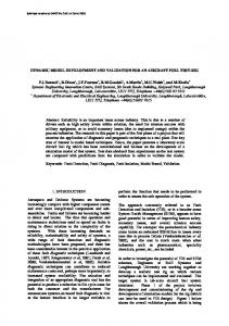
and 9.5 gpc (1 gpc corresponds to 1 US gallon -2 per 100 square feet, approximately 0.4 l.m . This is the unit currently used by the US Forest Service (USDA-FS) for representing the ground concentration of firefighting products, reason why it was maintained in this analysis). For the Marseille tests, the minimum values of each class of concentration considered were the -2 following: 0.5, 0.8, 1, 1.5, 2, 3 and 4 l.m . In terms of statistical analysis of the modelling results, and although there is not an acceptance criterion defined for the evaluation of aerial dropping models performance, a 10% value for the modulus of the percentage error (100% times the difference between the observed and the computed values normalized by the latter) has been used as a quality requirement by the USDA-FS for this type of applications. This analysis was complemented with the calculation of a set of metrics commonly applied on the evaluation of numerical model performance (Abramowitz and Stegun 1972; ASTM International 2000; Chang and Hanna 2005). Figure 1 shows an example for the comparison of ground patterns obtained by simulation and measurement for the Marseille and Marana drops. The position of the aircraft at the instant of release was not registered, reason why the locations of the modelled and measured patterns in the grid are not comparable. Generally speaking, ADM shows the expected distinctive behaviour for the Marseille and Marana tests due to the use of different discharge systems. In fact, ADM copes with the accumulation of product at the front of the pattern observed with conventional delivery system (Figure 1a). On the contrary, in constant flow delivery systems a nearly constant coverage level is present over the duration of the drop due to the action of a computer-controlled door system. This behaviour is also captured by the model, as shown in Figure 1b. The qualitative analysis of the entire dataset of drops showed that, in general, a good agreement between the shapes of the experimental and simulated patterns for each contour level was observed.

(a) 60

S6L3

C [l.m-2]

40

4

20

3

ADM 0 0

20

40

60

80

100

120

140

160

2

160

1.5 1

140

y [m]

0.8

120

0.5

Measurement 100 80

100

120

140

160

180

200

220

240

x [m]

(b) C [gpc] 100 M118 7.5

50

ADM 0

5.5

100

200

300

400

500

600

100

3.5 2.5 1.5

y [m] 50

0.75

Measurement 100

200

300

400

500

600

0.25

x [m]

Figure 1. Comparison between simulated and measured ground patterns of product concentration for the Marseille (a) and Marana (b) drop tests.

The quantitative analysis of modeling performance was made by the statistical analysis of the results for each drop. Table 2 presents the mean statistical metrics for the entire datasets of measured and simulated pattern length values according to Abramowitz and Stegun (1972), ASTM International (2000) and Chang and Hanna (2005). These parameters are the following: mean (µ), standard deviation (σ), average bias (d), geometric mean bias (MG), geometric variance (VG), fractional bias (FB), normalized mean squared error (NMSE), Pearson correlation coefficient (r) and factor of two (FAC2). Note that d is calculated from the difference between the measured and the simulated values.

From the statistical parameters given in Table 2 it is possible to conclude that the model exhibits a general good performance for both experiments, as indicated by the averaged NMSE of 0.01, which was found to be independent from viscosity. Both the µ and σ values over the computed dataset are in close agreement with the measured parameters, notwithstanding the slight tendency for underestimating the length of the ground patterns, as shown also by the positive value of the mean bias d. Apparently there is not an immediate relation between the tendency of the model to under- or overestimate the lengths of the contours per class of concentration and the meteorological conditions, although it was observed a model tendency for underestimating lengths in headwind drops. The modelling outputs were also statistically evaluated in terms of the area occupied by each coverage level. The results are presented in Table 3. Although the good correlation between model and measurement is maintained, there is an increase of the NMSE. This behaviour was observed in particular for the low viscosity drops in which, in accordance to the line lengths analysis, a slight tendency for underestimation is observed. Nevertheless, 94% and 88% of the data are within a factor of two of the observations for the Marseille and Marana simulations, respectively, as indicated by the FAC2 parameter. Table 3. Averaged statistical parameters for the evaluation of ground pattern area simulation. Area results evaluation Marseille Marana Measured ADM Measured ADM

µ (m)

Table 2. Averaged statistical parameters for the evaluation of ground pattern length simulation. Line length results evaluation Marseille Marana Measured ADM Measured ADM

µ (m)

σ (m) NMSE (-) r (-) d (m) MG (m) VG (m2) FB (-) FAC2 (-)

58.80

56.70

161.86

159.22

36.40

36.50

107.79

102.01

0.000

0.010

0.000

0.010

1.000

0.983

1.000

0.986

0.00

2.12

0.00

2.65

1.00

1.16

1.00

1.16

1.00

1.24

1.00

1.82

0.000

0.037

0.000

0.017

1.000

0.917

1.000

0.911

σ (m) NMSE (-) r (-) d (m) MG (m) VG (m2) FB (-) FAC2 (-)

694.96

692.11

2717.1

2588.3

635.82

621.73

2713.6

2587.2

0.000

0.020

0.000

0.040

1.000

0.991

1.000

0.981

0.00

2.84

0.00

128.77

1.00

1.09

1.00

1.11

1.00

1.32

1.00

1.52

0.000

0.004

0.000

0.049

1.000

0.938

1.000

0.877

The performance goal of the model is to guarantee that, for each contour level, the percentage error of the estimated line length values is lower than 10%. Figure 2 shows that 78% of the computed values fulfill this data

quality criterion. In fact, the error associated to the simulation of the pattern length in each concentration level is lower than 0.2% in 46% of the estimations. Fraction of values (%)

50 40

4 shows two examples for the comparison between the computed and measured Vx values. The position of the curves in the x-axis was adjusted in order to give the best fit (note that the position of the aircraft is unknown, and therefore the position of the pattern in the grid cannot be compared).

30 20

(a)

10

50

S6L3

Measurement ADM

0 [0, 0,2[

[0,2, 1[

[1, 10[

[10, 20[

[20, 50[

>50

40

Percentage error (%) 30

20

10

0 0

35

Simulated line length (m)

250

M118

Measurement ADM

20 15

100

5

80

0 0

20

200

25

10

40

150

30

120

S4L1 S4L3 S6L1 S6L2 S6L3 S3L1 S3L2

100

(b)

140

60

50

x (m)

Vx (l)

Additionally, in Figure 3 the regression lines for the comparative analysis between measured and simulated line lengths per coverage levels are shown. The underestimation of the length of mid range coverage levels contours is visible in some of the Marseille simulations. Nevertheless, there is a good correlation between measured and simulated values for both drop tests.

Vx (l)

Figure 2. Percentage error of the computed line lengths.

100

200

300

400

500

600

x (m)

Figure 4. Example for the comparison between modelled and measured values of cumulative volume deposited along the x-axis for the Marseille (a) and Marana (b) drop tests.

0 0

20

40

60

80

100

120

140

In the example shown in Figure 4a it can be observed that ADM underestimates one of the peak values of Vx. On the contrary, and benefiting from the knowledge of flow rate values, there is an enhanced fitting between the experimental and model curves in the Marana example (Figure 4b). Nevertheless, in general the modelled results were in good agreement with the measured values.

Measured line length (m)

Simulated line length (m)

400

300

M128 M134 M183 M114 M112 M120 M110 M109 M119 M117 M118

200

100

4

0 0

100

200

300

400

Measured line length (m)

Figure 3. Regression analysis of the measured and simulated line lengths for the Marseille and Marana drops.

An additional indication on the spatial variation of the volume deposited at ground is given by the representation along the x-axis of   the cumulative volume Vx  = V ( y ) . Figure  y   

∑

CONCLUSIONS In general, ADM allowed a good representation of the spatial distribution of product for the different coverage levels. The statistical validation of the results showed that the model accuracy is actually within the statistical uncertainty of the “cup-and-grid” sampling method. 78% of the computed line lengths per coverage level are within a 10% error in general, with an average NMSE of 0.01 and a Pearson correlation coefficient above 0.9 in both Marseille and Marana drop trials. The

accuracy of the simulated areas per level decreases to an average NMSE of 0.02 and 0.04, for the two drop trials respectively, although the good correlation remains. In all cases, nearly 90% of the results were within a factor of two of observations. Also, the geometric mean was between 1.1 (for area) and 1.2 (for line length). The accuracy of the simulations shows no strong relation with the corresponding viscosity, although better results are obtained in the range from 700 to 1100 cP. ADM provides a new insight on the importance of aerodynamic breakup mechanisms on the generation and behaviour of droplets of firefighting liquid, while maintaining the run-time on a feasible level. Due to its characteristics and performance, ADM is primarily indicated for application in the support to the development and testing of more efficient firefighting products, delivery systems or aerial discharge operations. Therefore this tool could also significantly reduce the cost of exhaustive real scale drop testing. ADM can potentially be used also in formation, training and demonstration activities with pilots, aerial resource coordinators, civil protection personnel or general firefighters. The user control over the input parameters allows the effect on ground pattern to be assessed for a wide range of dropping scenarios, avoiding the natural variability and irreproducibility of field conditions, and a better understanding of the multiple interrelated phenomena involved.

Acknowledgements A special acknowledgement to the United States Forest Service (USDA-FS) for providing the Marana drops dataset, and particularly to Eng. Ryan Becker (San Dimas Technology & Development Center, USDA-FS); to Eng. Greg Lovellette and to Eng. Cecilia Johnson (Missoula Technology and Development Center, USDA-FS). An acknowledgement also to Dr. Ian Harman (CSIRO, Australia) and Prof. Rolf Reitz (University of Wisconsin, US). The authors would like to acknowledge the financial support of the Luso-American Foundation (FLAD) and the Portuguese Ministry of Science, Technology and Higher Education, through the Foundation for Science and Technology, for the Post-Doc grant of J.H. Amorim (SFRH/BPD/48121/2008) and the national research project FUMEXP (PTDC/AMB/66707/2006). Also an acknowledgment for financial support of the European Commission through the research projects ACRE (ENV4-CT98-0729), ERAS

(EVG1-2001-00019) and EUFIRELAB (EVR1CT-2002-40028).

5 REFERENCES Abramowitz M., Stegun I.A., 1972: ‘Handbook of mathematical functions with formulas, graphs and mathematical tables.’ (National Bureau of Standards-Applied Mathematics Series 55: USA) ASTM International, 2000: ‘Standard guide for statistical evaluation of atmospheric dispersion model performance, D 6589 – 00.’ (ASTM International: USA) Beale J.C., Reitz R.D., 1999: Modeling spray atomization with the Kelvin Helmholtz/RayleighTaylor hybrid model. Atomization and Sprays 9, 623 650. Chang JC, Hanna SR, 2005: Technical descriptions and user’s guide for the BOOT statistical model evaluation software package, version 2.0. George Mason University and Harvard School of Public Health. (Fairfax, VA) Crowe C., Sommerfeld M., Tsuji Y., 1998: ‘Multiphase flows with droplets and particles.’ (CRC Press: Florida) Finnigan J., 2000: Turbulence in plant canopies. Annual Review of Fluid Mechanics 32, 519-571. Giroud F., Picard C., Arvieu P., Oegema P., 2002: An optimum use of retardant during the aerial fire fighting. In ‘Proceedings of the 4th International Conference on Forest Fire Research’, 18-23 November 2002, LusoCoimbra, Portugal. (Ed DX Viegas). CD ROM. (Millpress: Rotterdam) Haider A. and Levenspiel O., 1989: Drag coefficient and terminal velocity of spherical and nonspherical particles. Powder Technology 58, 63-70. Harman I. and Finnigan J., 2007: A simple unified theory for flow in the canopy and roughness sublayer. Boundary-Layer Meteorology 123(2), 339-363. Hsiang L.-P. and Faeth G.M., 1992: Near-limit drop deformation and secondary breakup. International Journal of Multiphase Flow 18(5), 635-652. Hsiang L.-P. and Faeth G.M., 1995: Drop deformation and breakup due to shock wave and steady disturbances. International Journal of Multiphase Flow 21(4), 545 560. Inoue E., 1963: The environment of plant surfaces. In ‘Environment control of plant growth’. (Ed LT Evans) pp. 23-32 (Academic Press: New York)

Lee C.S., Park S.W., 2002: An experimental and numerical study on fuel atomization characteristics of high-pressure diesel injection sprays. Fuel 81, 2417 2423. Lin S.P., Reitz R.D., 1998: Drop and spray formation from a liquid jet. Annual Review of Fluid Mechanics 30, 85-105. Liu H., 2000: ‘Science and engineering of droplets: fundamentals and applications.’ (William Andrew Inc.: NY) Madabhushi R.K., 2003: A model for numerical simulation of breakup of a liquid jet in crossflow. Atomization and Sprays 13. 413424. Monin A.S., Yaglom A.M., 1971: ‘Statistical fluid mechanics: Mechanisms of turbulence – Vol. 1.’ (The Massachusetts Institute of Technology (MIT) Press: Massachusetts) Morsi S.A. and Alexander A.J., 1972: An investigation of particle trajectories in twophase flow systems. J. Fluid Mech. 55(2), 193208. Physick W.L., Garratt J.R., 1995: Incorporation of a high-roughness lower boundary into a mesoscale model for studies of dry deposition over complex terrain. Boundary-Layer Meteorology 74, 55-71. Raju M.S., 2005: Numerical investigation of various atomization models in the modeling of a spray flame. National Aeronautics and Space Administration (NASA) Report E-15389. (Washington, US) Reitz R.D., 1987: Mechanisms of atomization processes in high-pressure vaporizing sprays. Atomization and Spray Technology 3, 309337.

Reitz R.D., Bracco F.V., 1982: Mechanism of atomization of a liquid jet. Physics of Fluids 25, 1730-1742. Simmons H.C., 1977: The correlation of dropsize distribution in fuel-nozzle sprays. Journal of Engineering for Gas Turbines and Power 99, 309-319. Swanson D.H., Luedecke A.D., Helvig T.N., Parduhn F.J., 1975: Development of user guidelines for selected retardant aircraft. Final report, contract 26-3332, 15 February 1975. Honeywell Inc., Government and Aeronautical Products Division. (Hopkins, MI) Swanson D.H., Luedecke A.D., Helvig T.N., Parduhn F.J., 1977. Supplement to development of user guidelines for selected retardant aircraft. Final report, contract 263332, April 1977. Honeywell Inc., Government and Aeronautical Products Division. (Hopkins, MI) Swanson D.H., Luedecke A.D., Helvig T.N., 1978: Experimental tank and gating system (ETAGS). Final report, contract 26-3425, 1 September 1978. Honeywell Inc., Government and Aeronautical Products Division. (Hopkins, MI) USEPA, 2004: User's guide for the AERMOD meteorological pre-processor (AERMET) Revised draft. US Environmental Protection Agency (USEPA), Office of Air Quality Planning and Standards Report EPA-454/B-03-002. (Research Triangle Park, North Carolina)