Constable one has been adopted for the highest temperatures, while a new, single-step .... rich, mostly unburned interior of the diesel spray, and a second one, ...
2010-01-0148
Development and validation of predictive emissions schemes for quasi-dimensional combustion models Federico Perini, Enrico Mattarelli, Fabrizio Paltrinieri
University of Modena and Reggio Emilia, Modena, Italy
ABSTRACT The paper presents the development and validation of phenomenological predictive schemes for quasidimensional modeling of pollutant emissions in direct injected Diesel engines. Models for nitric oxide (NO), carbon monoxide (CO), as well as soot and unburned hydrocarbons (HC) have been developed. All of them have been implemented into a DI Diesel engine simulation environment, previously developed by the authors, which features quasi-dimensional modeling of spray injection and evolution, air-fuel mixture formation, as well as auto-ignition and combustion. An extended Zel'dovich mechanism, which takes into account the three main, thermal-NO formation chemical reactions has been developed for predicting NO emissions. A simple, onereaction soot formation model has been implemented, while a new approach has been proposed for soot oxidation, which considers two different temperature ranges: the well-established Nagle and StricklandConstable one has been adopted for the highest temperatures, while a new, single-step reaction model has been implemented at the low temperatures. The model for carbon monoxide formation relies on five chemical reactions, whose kinetics are computed exploiting partial equilibrium assumptions, in a system of 11 species. Finally, hydrocarbon emissions have been modeled taking into account the effects of three main sources: fuel injected and mixed beyond the lean combustion limit, fuel yielded by the injector sac volume and nozzle holes, as well as overpenetrated fuel. A detailed comparison with experimental data from a high speed, direct injected diesel engine, carried on for both full and partial load and for a wide range of engine speeds, shows that the models are capable to predict the engine emissions with reasonable reliability.
INTRODUCTION Since the last years, diesel engine technology is undergoing considerable advances, and research is very active, as modern diesel engines couple high efficiency with constantly increasing environmental friendliness. For their design and optimization, many simulation tools are available as a support of the experimental efforts: among them, the most complete are 3D-CFD software codes coupled with chemical kinetics solvers, which nowadays allow full engine cycle simulation to be run in reasonable amounts of time. Nevertheless, due to the high computational resources required, these tools are more suitable during the design process final stages, where attention is focused on operating and geometric details, while instead simpler, 1D-CFD codes are widely adopted in the early phases, due to their intrinsic capability in modeling the entire engine system and for investigating the interactions among its components. On the other hand, the accuracy of lumped parameters codes is strongly related - especially when dealing with diesel combustion - to a high number of parameters which have to be calibrated on detailed experimental data. In particular, as well known, the combustion process in HSDI engines is strongly dependent on fuel jet atomization and mixing with the surrounding air. For overcoming these problems, a number of quasi-dimensional, multi-zone combustion models has been developed [1-7]. Following this approach, a simplified three-dimensional modeling of the spray zone is applied, introducing a proper number of parcels and radial zones. This approach features, at the same time, a satisfactorily accurate representation of injection, mixing and combustion, while requiring very limited computational resources with respect to full 3D-CFD. Research in the field of quasi-dimensional models is still Page 1 of 27
focusing on the reduction of calibration parameters, as well as on phenomenological modeling of pollutant emissions, usually based on empirical relations [2,3,14,25,26]. The development of reliable prediction tools for engines operated with alternative fuels, such as blends of diesel and ethanol or other vegetable fuels, as well as gaseous fuels [8-11], is recently gaining interest. In this paper, the development of four detailed schemes for the prediction of HSDI diesel engines most significant pollutants is presented and discussed, on the bases of well established models, and with some original features devoted to reduce their dependence on tuning parameters. In the following paragraph, the detailed description of the models for nitric oxide, as well as soot, unburned hydrocarbons and carbon monoxide as well as their implementation into the quasi-dimensional diesel engine simulation framework previously developed by the authors [7] is described. The results are then validated and compared to experimental data from a small-bore, high speed, direct injected diesel engine of current production.
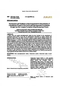
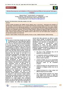
QUASI-DIMENSIONAL COMBUSTION MODEL Before going in depth into the development of the predictive models for pollutant emissions, the quasidimensional, multi-zone diesel combustion model previously developed by the authors [7] is introduced. This kind of simplified model – usually called quasi-dimensional, since the three-dimensional representation doesn't involve the whole cylinder, but is limited to the fuel spray jet – is able to predict engine performance with a high degree of accuracy, though requiring limited computational resources. As far as the fuel spray representation is concerned, a pictorial view on how it is generated is shown in Figure 1: finite packages (or 'parcels'), introduced at each computational timestep, represent fuel injected into the cylinder. Each parcel is then subdivided into a fixed number of radial and circumferential zones, which behave autonomously. More in detail, each single parcel in the present model is made up of 35 zones, corresponding to 5 radial and 7 circumferential subdivisions, respectively. After injection, and exploiting the usual presence of macroscopic charge motion, such as swirl, the spray dynamics are ruled by specific patterns, which are evaluated through empirical relations, while no momentum conservation equation is solved, thus reducing the computational efforts. As far as the evolution of the zones is concerned, specific models are included for computing both physical and chemical processes. First of all, the liquid column breaks up into a fuel spray; after the breakup process, air enters into the zone, and the liquid is atomized into droplets, whose diameter distribution is described in terms of estimated Sauter Mean Diameter. Then, evaporation may occur, being governed by ordinary thermodynamic balances. After ignition delay period for the mixture of air and fuel vapor is completed, combustion starts within the zone. Two types of combustion have been considered: a first premixed phase, where the fuel evaporated during the ignition delay is burnt; and a second diffusive combustion phase, ruled by a different Arrhenius-type kinetic equation. Lastly, the mass of burnt gases within the cylinder due to EGR is modeled as an inert thermal capacity. The detailed description of the multi-zone framework, as well as of relationships and calibration constants can be found in [7]. It is worth to mention that, thanks to some original details introduced in the model (i.e. finite-slab swirl and detailed turbulence modeling, comprehensive of the contributions due to injection and combustion), the model has proved to be reliable across a wide range of engine speeds and loads, and to undergo reduced dependence on calibration constants. As far as pollutant emissions are concerned, quasi-dimensional models are suitable for the implementation of even detailed schemes, due to the high resolution in modeling the spray zones, whose number can add up to 2000-3000 during the simulation of the power cycle of the engine. Each zone represents indeed a thermochemical system, in which equilibria and kinetic reactions occur and are solved. In the following, a detailed discussion of the four models developed for NO, soot, HC and CO estimation is proposed and described. Page 2 of 27
1 2 …
j
A n
(i,j)
i
Injection axis
A
PARCELS
A–A
ZONES
Figure 1 – Subdivision of fuel jet into parcels and zones.
NITRIC OXIDE FORMATION The minimization of NOx emissions is one of the most important targets which affect engine design and setup. For this reason, the formation of nitric oxides is under continuous investigation, as many detailed chemical kinetics mechanisms are still under development. It is generally acknowledged [31] that there are three major sources which concur to NOx formation in combustion systems: the first, usually called thermal-NO, is limited by a high activation energy, and thus is fast enough only at high temperatures; the second mechanism, of prompt or Fenimore NO, takes into account the formation of NO at the flame fronts, deriving from the recombination of the transient CH species. The last source is usually identified in the NO generated from the recombination of nitrous oxide (N2O), this contribution being significant especially for very lean mixture conditions and low temperatures. Most detailed diesel combustion kinetic mechanisms include full description of NO formation, where dozens species and reactions are involved [27]. In most phenomenological, multi-zone combustion models, instead, the three-dimensional description of the engine cylinder is simplified, and for this reason simple, equilibrium-based kinetics are usually adopted [2,3,14]. In this work, a similar approach has been followed, even if the NO formation model has been built in an expandable way, so that more complex mechanisms can be fit in the future. THERMAL NO – The extended Zel'dovich mechanism, made up of three reactions has been considered:
N 2 O NO N N O2 NO O ,
(1)
N OH NO H where the reaction rate of nitric oxide is expressed as an ODE: d [ NO ] cNO k f ,1[ N 2 ][O] kb ,1 [ NO ][ N ] dt k f , 2 [ N ][O2 ] kb , 2 [ NO ][O] k f ,3[ N ][OH ] kb ,3[ NO ][ H ]
Page 3 of 27
(2)
For the sake of reference, the coefficients of the forward reaction rates have been summed up in Table 1. The computation of the NO production rate relies on the knowledge of the concentrations of some other species, such as O, O2, N, H, and OH. Under the assumption of equilibrium for the dissociation of these species, their concentrations have been estimated by means of a chemical equilibrium program, which details are described more on. As a first attempt of understanding the behavior of the thermal-NO model, when coupled to a quasidimensional model, no more reactions have been included other than the Zel'dovich kernel mechanism. In particular, as far as the calibration process is concerned, a unique calibration constant, namely cNO, has been added to the forward reaction rate of the first reaction - see eq. (2). The assumption of modifying the rate limiting reaction has been considered as it is acknowledged that slight discrepancies from the Zel'dovich model can be caused by pressure effects in the equilibrium radical pool [27], and by the assumption that no mixing occurs among the zones [24]. b Table 1 – NO kinetics forward reactions rate coefficients in the Arrhenius-type form k A T exp E T , [31]. Units are cm, mol, s, K.
Reaction
A
b
E
1. N2+O NO+N
3.30E12 0.20
0.0
2. N+O2 NO+O
6.40E09 1.00
3160.0
3. N+OH NO+H
3.80E13 0.00
0.0
SOOT FORMATION AND OXIDATION The term soot is used to indicate the particulates formed during hydrocarbon combustion, when under substoichiometric conditions, for example due to poor air-fuel mixing [22]. Usually, soot emission models are subdivided into two parts: a first one, for computing primary soot particle formation, which takes place in the rich, mostly unburned interior of the diesel spray, and a second one, for estimating its following partial oxidation, occurring in the flame zone, when soot encounters molecular oxygen. Hence, the net soot formation rate is usually computed as the difference between formation and oxidation of soot: dms dms , f dms ,o . (3) dt dt dt
In this approach, a similar modus operandi has been followed; in particular, focusing on the behavior of the models available in literature for both the phenomena. Usually, [2,3,14,26], both submodels for soot formation and oxidation are tuned by means of two collision frequency values, which act as calibration parameters. In this approach, calibration is limited to the submodel of soot formation only, as the submodel for soot oxidation aims to be reliable at both low and high temperature ranges. In particular, the application of a combination of oxidation models has been addressed, providing satisfactory results, as well as a reduced dependence on model parameters. FORMATION OF SOOT – Soot formation and growth within an internal combustion engine occurs especially at high temperatures (over 1100K [22]). In most multi-zone, phenomenological combustion models [2,3,14], the soot formation process is represented as a one-way reaction between gaseous fuel and oxygen. This approach, Page 4 of 27
even if simple, is usually adopted due to the low computational effort required, and because of its empirical nature, which well suits simplified combustion models. Although, in full multidimensional engine simulations, often detailed fuel combustion chemistry is implemented [12], in which a more detailed – but still phenomenological – modeling of soot formation is included. In this paper, a first, one reaction soot formation model by Hiroyasu [3] has been implemented and tuned. This model features a soot formation rate computed as a first-order reaction of gaseous fuel and oxygen, as follows: dms , f dt
E As , f m f p 0.5 exp s , f RT
,
(4)
where Es,f is the activation energy, R is the universal gas constant, and the collision frequency As,f acts as a tuning parameter for fitting experimental data. As far as the activation energy is concerned, it is reported in literature to add up to either approximately Es,f = 5.234E4 kJ kmol-1 [14,26], or circa Es,f = 8.0E4 kJ kmol-1 [9,12]. In this study, the first of the two values has been chosen as reference. OXIDATION OF SOOT PARTICLES – As far as soot particles oxidation is concerned, only two different approaches can be found in the whole literature about quasi-dimensional combustion models. In particular, most of the combustion models apply a simple, one-way reaction model by Hiroyasu [3], while others exploit the semi-empirical relationship of Nagle and Strickland-Constable (NSC) [15], which relies on the hypothesis of two different oxidation sites: a more reactive one (A), and a less reactive (B), with thermal rearrangement between the sites ruled by an empirical rate constant. The approach of Hiroyasu is based on modeling of soot oxidation as a second-order reaction between molecular oxygen and soot (considered as gaseous): dms ,o E As ,o ms xO2 p1.8 exp s ,o , (5) dt RT
where the collision frequency factor, As,o, acts as a tuning constant for the oxidation model. A direct drawback of this approach is that the model is engine-dependent, since proper calibration has to be made for matching experimental soot measurements. The behavior of the Nagle and Strickland-Constable model, on the other hand, depends on the partial pressure of oxygen: it is a first order reaction for the lower values, and approaches zero at higher ones. This semiempirical formulation has proved to be suitable for high-temperature combustion [22]; for this reason, it is widely adopted in predictive engine combustion models. As previously introduced, two types of sites of oxidation are assumed to occur on soot particles [15], ruled by two different surface chemistry rates. Three chemical reactions are assumed to occur: kA
k A / kZ
Asite O2 surface oxide Asite 2CO kB
Bsite O2 Bsite 2CO kT
Asite Bsite
Page 5 of 27
(6)
Within this framework, the net soot oxidation rate is given by: k A pO dms ,o Wc 2 ms dt s ds 1 k Z pO2
x A k B pO 1 x A , (7) 2
where WC = 12 kg/kmol represents the molecular weight of carbon, ρs = 2 kg/dm3 the soot density, and ds = 1.0E-9 m the soot particle estimated diameter. The proportion between A and B sites is given by the fraction of A sites xA, which is computed as follows: xA
pO2 pO2 kT k B
.
(8)
As far as the rate constants of the NSC model are concerned, they only depend on the temperature of the mixture within the zone, and are computed as follows [15]: k A 20 exp 15100 T
g cm s atm g cm s atm g cm s atm 2
k B 4.46 E 3 exp 7640 T
2
kT 1.51E 5 exp 48800 T k Z 21.3 exp2060 T
2
.
(9)
1
A COUPLED OXIDATION APPROACH – Though all the phenomenological models in literature adopt either of the two models for soot oxidation here presented, still these models suffer massive dependence on calibration constants, which usually have to be tuned not only among different engines, but often also when dealing with different loads and rotating speeds. For this reason, a new approach, which couples two different reaction rate models – for high and low temperature ranges - is here presented with the aim of reducing the dependence of the soot oxidation framework on tuning parameters. As it is highlighted by Stanmore et al. [22], the NSC oxidation model is widely adopted within engine simulation codes, because it has been developed analyzing high temperature combustion (> 1700K). Nevertheless, as it has been pointed out by Park and Appleton [23], this model suffers some underestimation of the oxidation rate, so tending to loose validity at lower temperatures. For this reason, a hybrid oxidation model has been developed, which follows the NSC model for temperatures higher than 1700K, and a different, single-reaction oxidation model which has been defined and implemented for the lowest temperatures range. The formulation of the lower temperatures oxidation model (LTO) is an Arrhenius-type reaction equation:
dms ,o As ,o ms pO2 dt
E exp s ,o . RT
(10)
Following the analysis of the soot oxidation models in [22], the value for the low temperature activation energy has been assumed Es,o = 1.70E5 kJ/kmol, while the order of the reaction, expressed as the exponent on the reaction gas partial pressure pO2, has been chosen α=0.8. Similarly to that defined in Hiroyasu's model, a collision frequency As,o has been maintained; however, due to the different order of the reaction, it couldn't be regarded as a constant anymore, but has been determined for matching the NSC kinetic rate value at the temperature switch.
Page 6 of 27
In particular, the value for the collision frequency As,o has been calculated imposing equations (7) and (10) to yield the same value at Tswitch=1700K, being the expression always dependent on the partial pressure of oxygen:
As ,o
C
C1 pO2 2 pO2 1
pO2 2 C3 pO2 C4 C5 pO0.28
2
, (11)
C1 k A kT k Z T Tswitch C2 k Z kT T Tswitch
C3 k Z k B kT1 T Tswitch C4 1 k B T Tswitch
(12)
C5 exp Es ,o RT s d s T T
switch
Wc
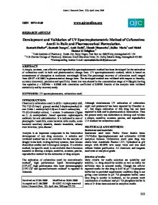
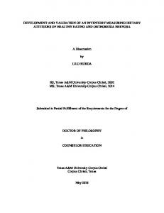
The constants C1, C2, ... C5 only depend on the switch temperature which separates the high and the low temperature ranges. In Figure 2, the so computed LTO collision frequency factor, normalized against the soot formation collision frequency As,f, has been plotted versus the molar fraction of oxygen within the zone, at the reference total pressure p = 120 bar. Figure 3, instead, shows the comparison among the considered soot oxidation models: the NSC model nonlinearly behaves on the Arrhenius plane, as the kinetic rate decreases in the high temperatures range; all the other one-reaction models, instead, are represented as a straight line. From the plot, it's clear that the combined approach NSC+LTO guarantees a higher oxidation rate in the low temperatures range than the simple NSC model, and it behaves similarly to most soot oxidation mechanisms, summarized by an averaged trend (cyan line with squares, in Figure 3) by Smith et al. [22]. Pressure dependence of LTO pre-exponential factor 200
As,o / As,f
150
100
50
0 0.1
0.15
0.2
0.25 0.3 0.35 O2 molar fraction, xO2
0.4
0.45
0.5
Figure 2 – LTO soot oxidation model collision frequency, normalized with respect to the soot formation collision frequency, vs. oxygen molar fraction, at the reference pressure p = 120 bar.
Page 7 of 27
Kinetic rates of soot oxidation
0
-1
log Rate (s )
5
-5
-10
NSC oxidation model [15] LTO oxidation model Ref. Jung [14] Ref. Smith [22] Temperature range switch
0.5
0.75 -1 -3 1/T (K x 10 )
1
1.25
Figure 3 – Arrhenius plot of the kinetic rates of soot gasification in air, following the two oxidation models considered in the soot model, in comparison with literature data, at the reference pressure p = 120 bar. The green line with diamond marks shows the kinetic law adopted by Jung and Assanis in [14]: it shows similar behavior with the NSC model at the extreme temperature values (>2000K,