Development and validation of the MC-Swift concept tire model

Development and validation of the MC-Swift concept tire model B.A.J. de Jong (0491090) DCT 2007.062

Master’s thesis Supervisor and member of graduation committee: Prof. Dr. H. Nijmeijer (Eindhoven University of Technology) Dr. Ir. I.J.M. Besselink (Eindhoven University of Technology / TNO Automotive) Ir. S.T.H. Jansen (TNO Automotive) Member of graduation committee: Dr. Ir. C.C.M. Luijten (Eindhoven University of Technology) Eindhoven University of Technology Department Mechanical Engineering Dynamics and Control Group Eindhoven, May, 2007

Samenvatting Om tegemoet te komen aan de vraag van de automotive industrie naar een goed bandmodel heeft TNO Automotive MF-Tyre/MF-Swift 6.0 ontwikkeld, een model dat het slip en relaxatie gedrag van een band beschrijft, maar daarnaast ook om kan gaan met wegoneffenheden van een korte golflengte en hoog frequente excitatie van de band dynamica. Omdat het model in eerste instantie ontwikkeld is voor autobanden, heeft het een aantal tekortkomingen in het geval van toepassing op motorfietsen. Deze tekortkomingen zitten voornamelijk in het verschil van camber hoek range tussen auto- en motorfietsbanden. Om tot verbeteringen van MF-Tyre/MF-Swift te komen voor motorfiets toepassingen is er allereerst een uitgebreid meetprogramma uitgevoerd. Het programma is gebaseerd op de standaard metingen die gedaan worden voor de parametrisering van MF-Tyre/MF-Swift aangevuld met camber hoek specifieke experimenten gevonden in de literatuur. De experimenten bestaan uit carcass stijfheidsmetingen, lage-snelheid enveloping metingen, slip gedrag tests en hoge-snelheid obstakel experimenten. De eerste twee metingen zijn uitgevoerd op de Flatplank test opstelling in Eindhoven en zijn uitvoerig beschreven. Wanneer het MF-Tyre/MF-Swift band model wordt geanalyseerd kunnen een aantal problemen onderscheiden worden. Allereerst wordt de dwarsdoorsnede van een motorfietsband beschreven door een ellips vorm, in tegenstelling tot een autoband. Hierdoor is ook de effectieve rolstraal camber hoek afhankelijk. Door de introductie van het dynamische gedrag van de band doormiddel van het Swift model ligt de focus van dit onderzoek daarnaast ook op het contact en enveloping model. Het contact model in het huidige MF-Tyre/MF-Swift is niet gecambered. In de literatuur is een beschrijving van een gecambered carcass band model gevonden, welke is gebruikt als basis voor ontwikkeling van een nieuw contact model voor het huidige TNO band model. Door een gecambered contact model worden de laterale en verticale stijfheid in het model benaderd door de radiale en axiale stijfheid van de band. Een nauwkeurige benadering van de verticale stijfheid leidt tot een goede benadering van de ashoogte, wat een belangrijke factor is in het weggedrag van een motorfiets. Daarnaast geeft een gecambered contact model de mogelijkheid om het bandgedrag onder grote camber hoeken beter te beschrijven. Het relaxatie gedrag is camber afhankelijk en ook de non-lagging effecten kunnen worden beschreven. Het enveloping model voor een motorfietsband heeft andere geometrische parameters dan van een autoband. Daarnaast is de contact lengte van de band camber hoek afhankelijk, wat een belangrijke factor is in het obstakel filter gedrag van het enveloping model. Om de voorgestelde ontwikkelingen te kunnen valideren is het MF-Tyre/MF-Swift model gereconstrueerd in Matlab/Simulink. Dit model wordt het MC-Swift concept bandmodel genoemd. Al de uitgevoerde metingen zijn gesimuleerd met dit model en met het originele MF-Tyre/MF-Swift 6.0 model voor verschillende camber hoeken. De resultaten zijn vergeleken met de metingen op basis van de ashoogte, non-lagging effecten, het relaxatie gedrag, enveloping gedrag en dynamische excitatie doormiddel van hoge-snelheid obstakel tests. Er kan worden geconcludeerd dat het MC-Swift concept model beter presteert met het gecamberde contact model. Daarnaast blijkt het dat de non-lagging effecten een belangrijke rol spelen in de metingen op de verschillende test opstellingen. Experimentele resultaten van de stijfheids, relaxatie en hoge-snelheid obstakel tests kunnen beter verklaard en benaderd worden door het introduceren van de non-lagging effecten in het bandmodel. Daarnaast is het enveloping model ook beter geworden.

i

Abstract To meet the demand from the automotive industry for tire models TNO Automotive has developed MF-Tyre/MF-Swift 6.0, a model widely used for car tire simulation. It describes the slip and relaxation behavior, but next to that it can also handle short wavelength road unevenness and other high-frequent excitation of the tire dynamics. Because the model is mainly developed for car tire simulation it has a few limitations with respect to motorcycle applications. These limitations are caused by the different operating range of a motorcycle tire compared to a car tire in terms of camber angle. To be able to develop improvements of the tire model for motorcycle applications, first of all an extensive test program is conducted. The measurements are based on the standard MF-Tyre/MFSwift program including test cases for large camber angles found in the literature. The experiments consist of static stiffness and low-speed enveloping tests, slip behavior measurements and high-speed obstacle tests. The static stiffness and low-speed enveloping tests are performed on the Flatplank test stand and are described in more detail. When the MF-Tyre/MF-Swift tire model is analyzed a couple of problems can be distinguished. First of all the cross section of a motorcycle is described by an ellipsoidal shape, in contradiction to a car tire. This also leads to a camber dependent effective rolling radius. Next to that, by introducing the dynamic behavior (Swift model) the focus of this research also lays on the contact and enveloping model. The current contact model in MF-Tyre/MF-Swift is not cambered. In the literature a description is found of a tire model with a cambered contact model. This is used as basis of the development of the new cambered contact model for the TNO tire model. By using a cambered contact model the lateral and vertical stiffness are approximated by the radial and lateral stiffness of the carcass of the tire. An accurate vertical stiffness determines the axle height of the tire better, which is an important factor in motorcycle simulation. Next to that, a cambered contact model gives the opportunity to better describe the tire behavior under large camber angles. The relaxation behavior is camber dependent and also the non-lagging effects for large camber angles can be approximated. The enveloping model for the motorcycle tire has different geometrical parameters compared to the car tire. Next to that, the contact length is camber dependent, which is an important factor in the obstacle filtering behavior of the enveloping model. To be able to validate the proposed changes, the MF-Tyre/MF-Swift code is reconstructed in a Matlab/Simulink model. This model is called the MC-Swift concept tire model. All the conducted measurements are simulated with this model and with the original MF-Tyre/MF-Swift 6.0 model for different camber angles. The models are compared with the measurement results on axle height, nonlagging effects, the relaxation behavior, enveloping behavior and high-speed obstacle response. It is concluded that the MC-Swift concept model performs better with the cambered contact model. It also appears that the non-lagging effects play an important role in the results obtained from the different test stands. Experimental results of stiffness, relaxation and high speed obstacle tests can be better explained and approximated with the introduction of the non-lagging effects in the tire model. Next to that the enveloping model performs better.

iii

Contents Samenvatting

i

Abstract

iii

Symbol and sign conventions

vii

1

Introduction 1.1 Background . . . . . . . . . . . . . . . . . . . . . . . . . . . . . . . . . . . . . . . . . . 1.2 Problem statement . . . . . . . . . . . . . . . . . . . . . . . . . . . . . . . . . . . . . . 1.3 Report layout . . . . . . . . . . . . . . . . . . . . . . . . . . . . . . . . . . . . . . . . .

2 Literature study 2.1 General tire modeling . . . . . . . . . . . . 2.1.1 Dynamic tire models . . . . . . . . 2.1.2 Motorcycle tire models . . . . . . . 2.2 The Pacejka based tire model development . 2.2.1 Dynamic tire models . . . . . . . . 2.2.2 Enveloping behavior . . . . . . . . . 2.2.3 Motorcycle tire models . . . . . . .

1 1 1 3

. . . . . . .

. . . . . . .

. . . . . . .

. . . . . . .

. . . . . . .

. . . . . . .

. . . . . . .

. . . . . . .

. . . . . . .

. . . . . . .

. . . . . . .

. . . . . . .

. . . . . . .

. . . . . . .

. . . . . . .

. . . . . . .

. . . . . . .

. . . . . . .

. . . . . . .

. . . . . . .

. . . . . . .

. . . . . . .

. . . . . . .

. . . . . . .

5 5 5 9 10 10 11 11

The tire experiments 3.1 Static tire carcass stiffness for zero camber . 3.2 Static tire carcass stiffness with camber . . 3.3 The relaxation behavior . . . . . . . . . . . 3.4 The enveloping behavior . . . . . . . . . . . 3.5 Tire footprint measurements . . . . . . . .

. . . . .

. . . . .

. . . . .

. . . . .

. . . . .

. . . . .

. . . . .

. . . . .

. . . . .

. . . . .

. . . . .

. . . . .

. . . . .

. . . . .

. . . . .

. . . . .

. . . . .

. . . . .

. . . . .

. . . . .

. . . . .

. . . . .

. . . . .

. . . . .

17 18 20 22 23 26

4 Analysis of MF-Tyre/MF-Swift 4.1 The current status of MF-Tyre/MF-Swift 6.0 4.2 Limitations and improvements . . . . . . . 4.2.1 The carcass stiffness/contact model 4.2.2 The enveloping model . . . . . . . .

. . . .

. . . .

. . . .

. . . .

. . . .

. . . .

. . . .

. . . .

. . . .

. . . .

. . . .

. . . .

. . . .

. . . .

. . . .

. . . .

. . . .

. . . .

. . . .

. . . .

. . . .

. . . .

. . . .

. . . .

29 29 29 30 34

The MC-Swift concept tire model 5.1 The rigid ring model . . . . . . . . . . . . . . . 5.2 The contact model . . . . . . . . . . . . . . . . 5.2.1 The shape of the cross section of the tire 5.2.2 The contact forces . . . . . . . . . . . . 5.2.3 The slip velocities . . . . . . . . . . . . 5.2.4 Describing the non-lagging effects . . . 5.3 The enveloping model . . . . . . . . . . . . . . 5.4 Summary . . . . . . . . . . . . . . . . . . . . .

. . . . . . . .

. . . . . . . .

. . . . . . . .

. . . . . . . .

. . . . . . . .

. . . . . . . .

. . . . . . . .

. . . . . . . .

. . . . . . . .

. . . . . . . .

. . . . . . . .

. . . . . . . .

. . . . . . . .

. . . . . . . .

. . . . . . . .

. . . . . . . .

. . . . . . . .

. . . . . . . .

. . . . . . . .

. . . . . . . .

. . . . . . . .

. . . . . . . .

37 39 42 42 44 46 47 50 52

3

5

v

vi

ABSTRACT

6 Comparison of both models with the measurements 6.1 Ellips shaped tire cross section and effective rolling radius 6.2 The loaded radius . . . . . . . . . . . . . . . . . . . . . . 6.3 Non-lagging tire forces and moments . . . . . . . . . . . 6.4 The relaxation behavior . . . . . . . . . . . . . . . . . . . 6.5 The enveloping behavior . . . . . . . . . . . . . . . . . . . 6.6 The dynamic behavior . . . . . . . . . . . . . . . . . . . . 7

. . . . . .

. . . . . .

. . . . . .

. . . . . .

. . . . . .

. . . . . .

. . . . . .

. . . . . .

. . . . . .

. . . . . .

. . . . . .

. . . . . .

. . . . . .

. . . . . .

. . . . . .

. . . . . .

53 54 55 56 58 60 62

Conclusions and recommendations 69 7.1 Conclusions . . . . . . . . . . . . . . . . . . . . . . . . . . . . . . . . . . . . . . . . . 69 7.2 Recommendations for future research . . . . . . . . . . . . . . . . . . . . . . . . . . . 71

Bibliography A The Magic Formula A.1 Slip characteristics . . . . . . . . . . A.1.1 Longitudinal force (pure slip) A.1.2 Lateral force (pure slip) . . . A.1.3 Aligning moment (pure slip) A.1.4 Overturning moment . . . . A.1.5 Rolling resistance moment . A.2 Tire model parameter determination

73 . . . . . . .

. . . . . . .

. . . . . . .

. . . . . . .

. . . . . . .

. . . . . . .

. . . . . . .

. . . . . . .

. . . . . . .

. . . . . . .

. . . . . . .

. . . . . . .

. . . . . . .

. . . . . . .

. . . . . . .

. . . . . . .

. . . . . . .

. . . . . . .

75 75 76 76 77 77 78 78

B Experiments B.1 Geometrical limitations of the Flatplank . . . . . . . . . B.2 The relaxation behavior . . . . . . . . . . . . . . . . . . B.3 The enveloping behavior . . . . . . . . . . . . . . . . . . B.4 MC-Swift parameter assessment measurement program

. . . .

. . . .

. . . .

. . . .

. . . .

. . . .

. . . .

. . . .

. . . .

. . . .

. . . .

. . . .

. . . .

. . . .

. . . .

. . . .

. . . .

81 81 83 84 86

C The MC-Swift concept tire model C.1 Test stand Simulink model . . . . . . . . . . . . . . . . . . . . . . . . . . . . . . . . . C.2 Contact model on a flat road surface . . . . . . . . . . . . . . . . . . . . . . . . . . . .

87 87 88

D Comparison of the models with the measurements D.1 Ellipsoidal cross section shape . . . . . . . . . . . . . . . . . . . . . . . . . . . . . . . D.2 Non-lagging effects of a statically loaded tire . . . . . . . . . . . . . . . . . . . . . . . . D.3 Dynamic behavior . . . . . . . . . . . . . . . . . . . . . . . . . . . . . . . . . . . . . .

89 89 90 93

. . . . . . .

. . . . . . .

. . . . . . .

. . . . . . .

. . . . . . .

. . . . . . .

. . . . . . .

. . . . . . .

. . . . . . .

. . . . . . .

Sign conventions In this report the translations and rotations are defined according to the right-handed ISO sign convention.

r e30

r e20

r e10

The axis of an arbitrary axis system are labeled as depicted above. These axes are defined with respect to the axis system ‘0’, which is placed in the superscript. The direction of the axis is labeled as subscript (1,2 or 3). This labeling sequence also holds for position and rotation vectors and their time-derivatives. Superscript 0 a b c r s θ

Description with respect to world axis system with respect to axle axis system with respect to belt (rigid ring) axis system with respect to contact model axis system with respect to road axis system with respect to slip axis system with respect to rotating axis system

Subscript 1 2 3

Description longitudinal (x) direction lateral/axial (y) direction vertical/radial (z) direction

To ensure unambiguously defined axis systems in all tire models and measurements the so-called TYDEX conventions are introduced by the tire (model) industry. Two axis systems are defined in TYDEX: The C-axis system, which is fixed in the wheel axle and is equal to the axle (‘a’) axis system in this report. Next to that the W-axis system is defined. This axis system is placed in the contact point and is equal to the road (‘r’) axis system in this report, with the XY-plane tangent to the road surface. All the different axis systems defined in this report are depicted in chapter 5.

vii

SYMBOL AND SIGN CONVENTIONS

vertical

viii

ra d

ia l

lateral

ax ial

For a better readability of the text the 2-direction (y) and 3-direction (z) in the local tire axis systems (‘a’, ‘b’, ‘c’) are called axial and radial respectively. In the global world (‘0’), slip (‘s’) and road (‘r’) axis systems these directions are called lateral and vertical respectively.

ix

Symbols Symbol Capital A1...6 C CF α0 CF αb CM αb CF κ0 Dy Fbx Fby Fbz Fcpe Fcx Fcy Fcz Fxw Fyw Fywss Fywnl Fz Fz0 Fzn Fzn0 Ia Ib Icz Mbx Mby Mbz Mcpe Mcz Qv R R0 R0y R0z Vbcx Vbcy Vbcz Vcpx Vcpy Vsx Vsy Vsy1 Vsy, ef f Vx Z Z1 Z2

Description empirically fitted non-lagging parameters load case (way of loading the tire) indication lateral slip stiffness lateral slip stiffness brush model aligning moment stiffness brush model longitudinal slip stiffness Magic Formula factor longitudinal rigid ring force axial rigid ring force radial rigid ring force force vector in contact patch elements longitudinal contact force axial contact force radial contact force longitudinal force in world coordinate system lateral force in world coordinate system steady-state lateral slip force in world coordinate system non-lagging lateral force in world coordinate system vertical load on tire nominal vertical load on tire vertical load on tire normal to the road initial vertical load on tire normal to the road inertia tensor of the axle inertia tensor of the belt yaw inertia of the contact body rigid ring overturning moment rigid ring roll moment rigid ring self-aligning moment moment vector in contact patch elements yaw contact moment deformation velocity scaling parameter for rigid ring stiffnesses load case (way of loading the tire) indication free rolling radius of tire undeformed axial distance between axle center and contact point undeformed radial distance between axle center and contact point longitudinal velocity rigid ring contact point axial velocity rigid ring contact point radial velocity rigid ring contact point longitudinal velocity of contact patch lateral velocity of contact patch longitudinal slip velocity in contact point lateral slip velocity in contact point lateral slip velocity in additional slip point effective lateral slip velocity longitudinal velocity load case (way of loading the tire) indication center height front ellips enveloping model center height rear ellips enveloping moddel

Unit [-] [-] [N.rad−1 ] [N.rad−1 ] [Nm.rad−1 ] [N] [-] [N] [N] [N] [N] [N] [N] [N] [N] [N] [N] [N] [N] [N] [N] [N] [kgm2 ] [kgm2 ] [kgm2 ] [Nm] [Nm] [Nm] [Nm] [Nm] [radms−1 ] [-] [m] [m] [m] [ms−1 ] [ms−1 ] [ms−1 ] [ms−1 ] [ms−1 ] [ms−1 ] [ms−1 ] [ms−1 ] [ms−1 ] [ms−1 ] [-] [m] [m]

x

SYMBOL AND SIGN CONVENTIONS Normal a b be bs cbx cbx0 cby cbz cbz0 cbγ cbθ cbθ0 cbψ cch ccpy ccx ccy ccz,0 ccz,1 ccψ ce crs crx cry crz crψ cresidual crigidring cs ctotal cγ cψ dzef f, wc dρr fco fr ha hobs hstep i kbx kby kbz kbγ kbθ kbψ krx kry krz krψ lb ls m ma mb mc n nc

half the contact length of the tire half the contact width of the tire longitudinal enveloping model ellips shape coefficient axial cross section ellips shape coefficient longitudinal rigid ring stiffness nominal longitudinal rigid ring stiffness axial rigid ring stiffness radial rigid ring stiffness nominal radial rigid ring stiffness rigid ring torsional camber stiffness rigid ring torsional wind-up stiffness rigid ring nominal torsional wind-up stiffness rigid ring torsional yaw stiffness total lateral stiffness carcass lateral contact patch elements stiffness total longitudinal carcass stiffness total axial carcass stiffness constant term in total radial carcass stiffness first order term in total radial carcass stiffness torsional yaw stiffness of carcass vertical ellips shape coefficient stiffness of spring representing the road surface residual longitudinal stiffness residual axial stiffness residual radial stiffness residual yaw stiffness residual stiffness in no specific direction rigid ring stiffness in no specific direction radial cross section ellips shape coefficient total carcass stiffness of tire in no specific direction torsional camber stiffness of carcass torsional yaw stiffness of carcass correction on vertical wheel centre displacement difference in radial deformation cut-off frequency rolling resistance coefficient axle height obstacle height height of step obstacle contact point grid number enveloping model rigid ring longitudinal damping constant rigid ring axial damping constant rigid ring radial damping constant rigid ring torsional camber damping constant rigid ring torsional wind-up damping constant rigid ring torsional yaw damping constant residual longitudinal damping constant residual axial damping constant residual radial damping constant residual yaw damping constant length of elliptical curve enveloping model tandem length enveloping model adhesion factor of contact patch mass of the axle mass of the belt mass of contact body number of grid points in ellips enveloping model number of cams per tandem in enveloping model

[m] [m] [m] [m] [Nm−1 ] [Nm−1 ] [Nm−1 ] [Nm−1 ] [Nm−1 ] [Nm.rad−1 ] [Nm.rad−1 ] [Nm.rad−1 ] [Nm.rad−1 ] [Nm−1 ] [Nm−1 ] [Nm−1 ] [Nm−1 ] [Nm−1 ] [Nm−2 ] [Nm.rad−1 ] [m] [m] [Nm−1 ] [Nm−1 ] [Nm−1 ] [Nm.rad−1 ] [Nm−1 ] [Nm−1 ] [m] [Nm−1 ] [Nm.rad−1 ] [Nm.rad−1 ] [mm] [mm] [Hz] [-] [m] [mm] [mm] [-] [Nsm−1 ] [Nsm−1 ] [Nsm−1 ] [Ns.rad−1 ] [Ns.rad−1 ] [Ns.rad−1 ] [Nsm−1 ] [Nsm−1 ] [Nsm−1 ] [Ns.rad−1 ] [m] [m] [-] [kg] [kg] [kg] [-] [-]

xi nt pbe pce qa1 qa2 qbV x qbV z qbV θ re rll rlr rsy u v w x xa xb xc xrb xrc y0 ya yb ycp yrb yrc z0 za zb zcm zef f zrb zrc Greek α βr βx βy γ γa γrb εc εlim ζy νrs θ θa θrb κ ρr ρy σb σc σy τc ψa ψrb ψrc Ωa

number of parallel tandems in enveloping model scaling parameter longitudinal ellips shape coefficient scaling parameter vertical ellips shape coefficient first order term in contact length as function of normal force second order term in contact length as function of normal force scaling factor longitudinal rigid ring stiffness scaling factor radial rigid ring stiffness scaling factor torsional wind-up rigid ring stiffness effective rolling radius axial part of loaded radius radial part of loaded radius additional slip point radius longitudinal deformation contact patch elements lateral deformation contact patch elements (effective) road height traveled longitudinal distance longitudinal position of axle center longitudinal velocity rigid ring center contact point position on ellips enveloping model longitudinal rigid ring deformation longitudinal residual deformation local y-coordinate cross section shape ellips lateral position of axle center axial velocity rigid ring center lateral displacement contact patch axial rigid ring deformation axial residual deformation local z-coordinate cross section shape ellips height of axle center radial velocity rigid ring center height of contact body effective road height radial rigid ring deformation radial residual deformation lateral slip angle of tire rolling resistance angle (effective) inclination angle of the road (effective) forward road slope camber angle of the tire camber angle of the axle rigid ring camber deformation non-lagging slip speed ratio limit value of rel. length contact patch elements equivalent transient side-slip compression of spring representing the road surface tire composite parameter rotation angle of the axle rigid ring wind-up deformation longitudinal slip coefficient radial deformation of the tire axial deformation of the tire lateral relaxation length brush model lateral relaxation length contact patch elements lateral relaxation length relaxation time-constant yaw angle of the axle rigid ring yaw deformation contact body yaw angle with respect to rigid ring rotation velocity of the axle

[-] [-] [-] [mmN−0.5 ] [mmN−1 ] [Nsm−2 .rad−1 ] [Nsm−2 .rad−1 ] [Ns.rad−2 ] [m] [m] [m] [m] [m] [m] [m] [m] [m] [ms−1 ] [m] [m] [m] [m] [m] [ms−1 ] [ms−1 ] [m] [m] [m] [m] [ms−1 ] [m] [m] [m] [m] [rad] [rad] [rad] [rad] [rad] [rad] [rad] [-] [m] [rad] [m] [-] [rad] [rad] [-] [mm] [mm] [m] [m] [m] [s] [rad] [rad] [rad] [rads−1 ]

xii

SYMBOL AND SIGN CONVENTIONS

Chapter 1

Introduction 1.1

Background

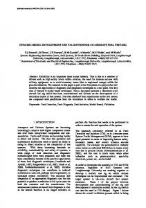
During the design period of a road vehicle, simulation has become an increasingly important part of the process. Because of the enormous increase in computer power more detailed and complex simulations can be done. This so-called virtual prototyping saves a lot of valuable testing time. To be able to simulate the dynamic behavior of the vehicle or motorcycle a detailed tire model is needed, which describes the interaction of the tires with the road given certain inputs like steer angle, brake input and road surface. Especially with single track vehicles like motorcycles a good tire model is important. Straight line and cornering stability are major issues for this kind of vehicles and the tire behavior plays an important role in this area. In the late eighties tire modeling firstly concentrated on car tires, because the automotive branch was leading in research and development with respect to motorcycle manufacturers in that time. Next to that, motorcycle modeling always has been more complicated which also has led to a smaller demand. At the TU Delft, in cooperation with few automotive companies, the so-called Magic Formula has been developed. The Magic Formula is a semi-empirical formula to describe the slip behavior of the tire. In 1996 this model was introduced on the commercial market by TNO-Automotive as MF-Tyre. Later on MF-Tyre has been extended with the SWIFT-model (Short Wavelength Intermediate Frequency Tyre - model) to describe the high frequency response, up to about 100 Hz, of the tire. Swift consists of a rigid ring model representing the tire belt body connected with spring/damper combinations to the axle. The mass of the belt and the spring/damper constants are tuned such that the rigid body modes of the tire are described accurately. Next to the rigid ring a road contact model has been introduced to describe the tire enveloping behavior over (discrete) 2D and 3D obstacles. MF-Tyre extended with Swift is called MF-Tyre/MF-Swift. Later on also the demand for tire models from the motorcycle industry has increased. Due to the completely different operating range of a motorcycle tire in terms of slip and camber angle compared to a car tire (see figure 1.1), the car tire slip model has to be revised in a couple of areas. Changes are developed for the Magic Formula to be able to handle large camber angles. Although the car Magic Formula has been the basis for the development of the motorcycle Magic Formula, the differences between the two models do not allow interchange of tire coefficients. The steady-state slip behavior of a motorcycle tire is described accurately in this way. However, for the contact model and the SWIFT extension of the tire model no analysis is done yet for a motorcycle tire application. In cooperation with Honda ASAKA and Bridgestone, TNO-Automotive has started a project to improve these parts of the MF-Tyre/MF-Swift tire model.

1.2

Problem statement

The commercial MF-Tyre/MF-Swift model is developed for car tires, and therefore it is possibly less suited for motorcycle tires. Especially large camber angles could prove to be a problem. The model 1

2

CHAPTER 1. INTRODUCTION

45

Camber angle [deg]

Motorcycles

30

Automobiles

15

5

10

Slip angle [deg]

Figure 1.1: The different operating ranges of a motorcycle and car tire

consists of four major subroutines. To be able to analyse the model in a clear manner, a distinction is made in these four subroutines. These are: • slip model (Magic Formula, slip forces) • carcass stiffness model (road contact model, contact forces) • short wavelength obstacle enveloping model (filtering short wavelength obstacles) • dynamic behavior model (tire belt vibration modes up to 100 Hz) As mentioned in the first paragraph the Magic Formula, which forms the slip routine of the model, is modified for the different operating range of motorcycle tires and the steady-state force and moment behavior is described accurately. The goal of this thesis is to analyze the other three routines for large camber angles and to propose possible improvements. With these improvements the tire model should be able to even better fit camber dependent Flatplank stiffness and low-speed cleat measurements as well as high speed obstacle tests for large camber angles. In a Matlab/Simulink model the four subroutines of MF-Tyre/MF-Swift, with the proposed adjustments, are reconstructed and they form the concept tire model. This model is used to simulate the performed measurements on the Flatplank at the Eindhoven University of Technology and the high speed cleat tests. Therefore also models of these test facilities are developed to be able to copy the experimental environments and to compare the measurement results with simulation results thoroughly. This analysis includes: • the axle height • the non-lagging lateral force • the relaxation behavior • the enveloping behavior • the dynamic behavior

1.3. REPORT LAYOUT

1.3

3

Report layout

First of all a literature survey is done to get insight in the current knowledge and research performed on dynamic and motorcycle tire modeling. General tire behavior from test and simulations found in the literature can also be used to compare with simulation results of the developments in the concept tire model. In chapter 3 the test program is described. The test program consists of measurements done by TNO and the experiments done at the Eindhoven University of Technology, which are treated in more detail. A standard measurement program for MF-Tyre/MF-Swift is performed. However, the camber range is larger as for car tires. This also leads to more specific motorcycle tire measurements as already found in the literature, which normally are not included in a standard data test. The measurements are used for parameter assessment as well as for model development. Relevant results are shown and analyzed. The current version of the TNO tire model, MF-Tyre/MF-Swift 6.0, is briefly analyzed and the limitations for motorcycle application are outlined in chapter 4. Also proposals for modifications are explained and to which improvements these have to lead. Then, in chapter 5 the new tire model, called the MC-Swift concept tire model, as developed in Simulink is depicted. This model contains the new developments as described in chapter 4. The implementation of these developments is treated. This model is used to test all proposed changes in the tire model and to validate these with the measurements and the original MF-Tyre/MF-Swift 6.0 tire model. After that, in chapter 6, the comparison between the MF-Tyre/MF-Swift 6.0 and the MC-Swift concept tire model is shown together with the validation of the models using the measurements. Differences are analyzed and explained. Finally conclusions are drawn about the proposed changes and recommendations are given for future research.

4

CHAPTER 1. INTRODUCTION

Chapter 2

Literature study Studying the already existing knowledge on dynamic tire models is a good starting point for developing a new tire model. Also the validity of the new model can be assessed by looking at similar research. This literature study is divided into two parts. Because this report will concentrate on the tire model of TNO, which is developed in the Pacejka research group, all research within this group is summarized in one paragraph. The first section concentrates on the general tire research done by other parties. Because the steady-state slip behavior forms the basics for every tire model both sections start with a short historic view on this subject.

2.1 2.1.1

General tire modeling Dynamic tire models

In 1956 Temple was the first to describe his ideas on steady-state tire modeling. Until then tires where seen as constraints on the movement of a vehicle and not as force producers. After that a lot of research is done on steady-state tire modeling, which later on also has concentrated on the dynamic behavior of the tire. From the past decades it has followed that there are three general ways to model the dynamic behavior of a tire. First of all the lumped parameter model is a commonly used approach. A lumped parameter model is a super simplified tire model where the tread of the tire is represented by an (elastic) string/beam/ring supported on a (visco) elastic foundation representing the sidewall. The rigid ring dynamic model is such a so-called lumped parameter model. Bruni discussed the vehicle comfort, braking and driving analysis with this model. Experiments have been carried out on a drum with a generic obstacle shape to determine the physical parameters of the model by considering the vertical and longitudinal axle forces on coast-down conditions (natural deceleration of the tire). Allison and Sharp also used the rigid ring model. The low frequent (up to 100 Hz) longitudinal in-plane vibration problems of vehicles are examined. Next to that, Takayama and Yamagishi [23] also modeled the carcass as a rigid ring. The model is used to analyze the tangential and radial axial forces that result from a tire hitting a cleat. Deflections from the cleat are absorbed by a vertical line spring and drive and roll resistance forces of the test wheel are absorbed by a horizontal spring in the rigid ring model. Calculated results agreed well with experimental results. As can be seen the rigid ring model is used to approximate all sorts of dynamic behavior tests of the tire. Another example of a lumped parameter model is proposed by Kim and Savkoor [11]. They have developed a model which consists of a thin circular elastic ring which is restrained by a continuous annulus of spring-damper elements. These elements act both in the radial and tangential direction and represent the membrane stiffness of the inflated torus enclosed by the carcass and the stiffness of the sidewall structure of the tire. An auxiliary elastic foundation with spring elements is attached to the outer ring surface to represent the radial and tangential flexibility of the tread rubber elements of the tire. The model is used to study the slip and traction distribution within the footprint of a 5

6

CHAPTER 2. LITERATURE STUDY

rolling tire, next to the design functions of supporting loads and cushioning road irregularities. Also interesting design requirements are the rolling resistance and tire wear. Loo [12] also describes a flexible ring model. This model consists of a flexible circular ring under tension with a nest of radially arranged linear springs and dampers (see figure 2.1). The aim of the

Figure 2.1: Flexible ring tire model [12]

model is to predict the tire’s vertical load deflection characteristics and its rolling resistance. The ring, which represents the tire belt, is assumed to be massless and completely flexible. The tension of the ring and the radial foundation stiffnesses, which depend on the inflation pressure of the tire, are determined by measuring the contact patch length and by doing static load tests. Eichler [5] has presented an elastic 1-ring belt model as can be seen in figure 2.2. The tire belt is modeled as a ring that

Figure 2.2: Elastic 1-ring belt tire model [5]

consists of a number of mass points interconnected by tensional and torsional springs to represent the tensile and bending stiffness. The torsional springs cγ and cφ represent the sidewall stiffness and the resistance of the belt to transverse displacement with respect to the rim. Next to the lumped parameter models a semi-analytical model approach can be distinguished. These hybrid models have been used in the earlier years because of the limited computational power and are regarded as a coarse FEM model approach. They are partly analyzed by a FEM algorithm, other parts of the model are simplified as with the lumped parameter models. Mastinu and Pairana [15] have employed a simple brush model combined with a finite-element (FE) algorithm. The FE algorithm computes the lateral deformation of the tire belt. The brush model computes the steady-state

2.1. GENERAL TIRE MODELING

7

longitudinal- and lateral force and self-aligning moment. This model is not able to describe the dynamical modes of the tire. Gipser [14] has developed the so-called BRIT model (see figure 2.3), the brush and ring tire model. A rigid ring is connected to the rim by massless elements with 6 degrees of freedom. The stress

Figure 2.3: BRIT model [14] distribution properties in the elements of the contact patch are determined with a FE approach. This model is able to determine the dynamical tire forces and moments response to road unevenness. Next to that Gipser also developed F-tyre [7]. In this model the belt is represented by 80 - 200 lumped mass nodes connected to the rim and each other by several nonlinear inflation-pressure-dependent stiffness, damping and friction elements. Each mass nodes has at least 5 degrees of freedom (see figure 2.4). It can be used for ride and handling analysis in steady-state and dynamic simulation. However, there

Figure 2.4: FTyre: degrees of freedom of the belt segments are limitations on the road surface input in terms of wave length. It also appeared from comparisons with measurement results that the calculated handling forces are not very accurate. Mastinu et al. [6] have introduced a semi-analytical model to describe the force-generation in the contact patch. The pneumatic tire is described by non-linear elastic elements connected to the rim and the tread pattern is modeled as linear longitudinal and lateral elastic elements as can be seen in figure 2.5. Finally, a lot of research is done on full finite-element models. These models demand a high computing power, but they also represent the real physical tire the best. Kao and Muthukrishan [10] have created a full FE model of a tire, with which it is possible to predict the tire dynamic response from the tire design data (geometry, material properties, fibre reinforcements, layout). Also the enveloping of the tire on obstacles can be observed very accurately (see figure 2.6). The whole model consists of 9600 elements and has 70800 degrees of freedom. This model is used in a simulation of an experiment on a rotating test drum with a cleat mounted on it. This experiment is also carried out in

8


Figure 2.5: Mastinu tire model [6]

Figure 2.6: tire enveloping of a FE model [10]

reality and the results are compared. From this comparison it can be concluded that the model shows a reasonable similarity with the real physical tire. Another commonly used full FE approach is the so-called membrane model. Such models require less nodes to obtain the same accuracy compared to the ordinary solid element models and therefore need less computing power. The carcass of the tire is modeled with membrane or shell elements as can be seen in figure 2.7. These shell elements are 2D, but they can be used as 3D elements because they can be given a certain width without adding nodes. Rhyne et al. [24] for example have proposed such a model. Their research focussed on the effect of rim imperfections like geometrical variations on the ride comfort and the resulting vertical force variation at the wheel axle. Scavuzzo et al. [19] used a membrane model to study the influence of the tire vibration modes on vehicle ride quality. They mainly have looked at the effect on these modes of parameters like tire size, tire construction, inflation pressure and operation conditions such as velocity, load and temperature. Simulations have been done with road irregularities like single impact bumps or chuckholes, but also with a series of small impacts from rough road surfaces. A lot of FEM software packages contain general purpose finite element tire models. Examples of these packages are ABAQUS and NASTRAN. These models have a good performance on dynamic tire behavior and are also used for tire noise modeling and analysis.

2.1. GENERAL TIRE MODELING

9

Figure 2.7: The membrane tire model

2.1.2

Motorcycle tire models

As described in the introduction the operating range of a motorcycle tire differs a lot from that of a car tire. Also the shape of the cross section of the tire is different. A car tire has an almost square cross section, however that of a motorcycle is round or elliptical shaped. This leads to a shift of the contact point when a tire is cambered. Lot [13] developed a motorcycle tire model in which the shape of the cross section is described. The forces on the tire are applied in the actual contact point. These forces are calculated with the basic uncombined Magic Formula and the instantaneous slip quantities in the actual contact point are used as input. This approach is closer to the physical tire behavior. To describe both the radial and axial stiffness and the resulting deformations of the tire when applying the forces in the actual contact point Lot developed a model as can be seen in figure 2.8. It can be seen that a normal force not only gives a radial deformation of the tire, but also an axial

Figure 2.8: The model developed by Lot to describe the carcass stiffnesses of the tire [13] deformation, due to the constraints imposed by the carcass spring model. This is different compared to the Pacejka models, where the axial deformation is not dependent on the vertical deformation and

10


vice versa. The relaxation of the carcass is incorporated in the model. This is achieved by taking the additional movement of the contact point due to the rolling on the contour of the motorcycle tire and the deformation of the tire in radial, tangential and lateral direction into account in the slip quantities. This is also an important difference with the Pacejka models. The equations for the slip quantities are linearized for small angles. Lot shows with sideslip and camber sweep measurements on the so-called DIM tire Meter Machine that this so-called linearized instantaneous slip model performs better than the transient tire model, with the standard first order relaxation filter. These results can be seen in figure 2.9. For the side slip experiments the same results are obtained for both models, but when

Figure 2.9: Comparison of real tire with the transient and instantaneous model [13] superimposing a camber angle on the wheel the instantaneous model shows no phase lag between the camber angle and lateral force. This also appears for the experiment with the real tire, while the transient model does show a phase lag for this experiment.

2.2 2.2.1

The Pacejka based tire model development Dynamic tire models

In 1987 H.B. Pacejka [2] introduced the Magic Formula for car tires. This model contains a set of mathematical formulae, partly based on empirical data and partly based on a physical background. After its first introduction, the Magic Formula has quickly gained a broad acceptance in the automotive industry for describing the non-linear steady-state force and moment reaction of a tire under combined slip conditions. By introducing the relaxation length of the tire the Magic Formula is able to describe the behavior up to 8 Hz accurately [17]. In 1997 the Magic Formula has been adapted by De Vries [4] to describe the steady-state behavior of motorcycle tires by introducing the effect of large camber angles. This formed the basis for the motorcycle Magic Formula, MF-MCTyre. For more and the latest information on the topic of steady-state tire modeling (Magic Formula) it is referred to [18]. In the early nineties a project was started at Delft University of Technology to develop a tire handling model that can be used for simulations with electronic control systems like anti-lock brake systems (ABS), traction control (ASR, TCS) and active yaw control systems (ESP, VDC). To be able to do reliable simulations with these systems the tire behavior has to be described for frequencies up to 30 Hz and for shorter wavelengths of the road surface. This project was carried out in close cooperation with TNO Automotive and nine automotive companies. Eventually this has resulted in the SWIFT

2.2. THE PACEJKA BASED TIRE MODEL DEVELOPMENT

11

(Short Wavelength Intermediate Frequency tire) model. This rigid ring tire model is able to describe the in-plane (longitudinal and vertical) and out-of-plane (lateral and yaw) tire behavior up to frequencies of 60 - 100 Hz [3]. The rigid ring model (see figure 2.10) consists of a rigid ring, which represents the tire belt, and this ring is suspended to the rim by spring-damper elements, which represent the sidewalls with pressurized air. Because the tire belt is modeled as a rigid body this model is only valid

Figure 2.10: Rigid ring tire model [21] for the rigid body modes of the tire. This means that only the primary modes are described and that the flexible belt modes are neglected. Other experimental approaches with the same rigid ring tire model are described by Bruni et al. [20] and Allison and Sharp [1].

2.2.2

Enveloping behavior

When a model with a single contact point is proposed, like the rigid ring model in the SWIFT tire model, also a model to describe the enveloping behavior of the tire on an obstacle is needed. This has an important influence on the excitation of the (dynamical) model. The enveloping model describes an effective road input for a single contact point, representing the tire reaction with a finite contact patch length rolling over an obstacle. The SWIFT-model for example is able to deal with short wavelengths of the road surface by using a contact model moving over empirically determined obstacle specific basic curves developed by Zegelaar [27] in 1998. Later this approach has been extended by Schmeitz [21] to describe the enveloping behavior of the tire over any arbitrary obstacle by a tandem model with elliptical cams which can be seen in figure 2.11. When a tire is rolling over an obstacle it appears that the radial stiffness of the tire at the front end and the rear end of the contact patch is much higher than at the center of the contact patch. Therefore, this enveloping model consists of two elliptical shapes describing the tire shape at the front and rear edge separated by a distance related to the contact patch length of the tire. For car tires this ratio is typically equal to 80% of the contact length. The effective road input described by this model is determined by averaging the height of both cams for every position on the obstacle. Also the effective road inclination angle can be determined. In figure 2.12 an effective road description can be seen for a step obstacle of 10 mm. This method is described in much more detail in [21].

2.2.3

Motorcycle tire models

Pacejka [17] describes the so-called non-lagging effects of a motorcycle tire for large camber angles. This non-lagging effect is a lateral force delivered by the tire due to the deformation of the carcass. It appears from this literature that the non-lagging lateral force, next to the normal load and camber angle, is also dependent on the way the tire is loaded. This means that the order of cambering and

12


Figure 2.11: The enveloping model described by Schmeitz [21]

Figure 2.12: Example of the description of an effective road for an step obstacle of 10 mm [21]

loading of the tire is important. Three load cases are described: first cambering and then loading the tire along the line perpendicular to the road surface (case Z), first cambering and then loading the tire along the line perpendicular to the horizontal wheel plane (radial loading, case R) and first loading and then cambering the tire (case C). The three cases are depicted in figure 3.4. Pacejka also introduces a

Figure 2.13: The three different load cases affecting the non-lagging lateral tire force [18]


13

model to describe the non-lagging part. It is stated that a tire response due to loading and/or tilting of the wheel while the longitudinal velocity Vx = 0 is the result of the integrated lateral velocity of the lower part of the wheel. A new slip point at a radius rsy is introduced, which is used as an additional component of the effective lateral slip speed Vsy, ef f . This can be seen in figure 2.14. The radius rsy is obtained by fitting a function proposed by Pacejka. It holds that:

Figure 2.14: The newly introduced slip point to approximate the non-lagging effects for different load cases [18]

Vsy, ef f = εc Vsy + (1 − εc )Vsy1

(2.1)

where: εc =

1 − A4 |γ| 1 + A5 Fz /Fz0 + A6 (Fz /Fz0 )2

(2.2)

The parameters A1 ...A6 are determined by a fitting procedure. With this approach the different responses of the non-lagging part for different load cases are handled. It can be seen from figure 2.14 that for case Z it holds that Vsy1 = 0 and Vsy = Vaz tan(γ). For case R Vsy = 0 and Vsy1 = −Vaz tan(γ) and for case C Vsy = 0 and Vsy1 = 0. Now, with the differences in the effective slip speed the deviations in the non-lagging response of the tire are tried to be explained. The computed non-lagging part of the side force shows reasonable correspondence with the experimental results of Higuchi [9]. Higuchi and Pacejka [9] describe a linear and non-linear relaxation model. Next to that, also measurements are performed on the non-lagging effects of the tire and a non-lagging part ratio is introduced. This is the ratio between the non-lagging lateral force and the steady-state lateral slip force. This ratio is dependent on the normal load, the camber angle and the load case as can be seen in figure 2.15. It is also shown by means of carcass deformation that a rolling cambered tire induces a lateral force without having a side-slip angle. Namely, due to the length of the contact patch a material point of the tire touching the road at the back edge of the contact patch tends to move laterally because of the camber angle of the wheel. However, because the material point is already touching the road surface it does not move because of friction and a lateral carcass deformation appears. This deformation induces a lagging lateral force. The space constant σy of this lagging force part is shown for different normal loads in figure 2.15. In [9] also the difference is shown of the linearized model and the non-linear model compared to experiments on the Flat Planck Tire Tester. Especially for a tire under a camber angle the non-linear model approximates the experiments very good, where the linearized model gives differences up to 50% for the lateral force. Maurice [16] has described a brush model attached to a flexible carcass. The brush model is coupled with two parallel springs at the two ends of the contact patch (see figure 2.16). Next to a lateral

non−lagging part ratio (−)


0

0



space constant tau (m)

14

1

0.5

0 −15

−10 −5 camber angle (deg) case R

1 0.5 0 −0.5 −1 −15

−10 −5 camber angle (deg)

case C 1

Fz = 2000 N

0.5

Fz = 4000 N

0

Fz = 6000 N

−0.5 −1 −15

−10 −5 camber angle (deg) case C

0

−10 −5 camber angle (deg)

0

1 0.5 0 −0.5 −1 −15

Figure 2.15: The lagging constant and the non-lagging part ratio are dependent on the camber angle, the normal load and the load case [18]

Figure 2.16: The brush model coupled with two parallel springs representing the carcass stiffness [16]

deflection of the carcass, also a torsional deflection appears when the lateral force is not acting in the center plane of the tire. This happens due to the pneumatic trail of the tire. Maurice gives the first-order differential equation derived from the brush model that gives a good approximation of the lateral tire response to side slip variations: H F y , αb =

CF αb σb jωs + 1

(2.3)

Now, because the relaxation length of the brush model σb underestimates the real relaxation length, the new relaxation length is derived for the model with the flexible carcass. To be able do to that a first


15

order approximation is used for the aligning moment. For the new relaxation length it then follows: σ=

ccψ CF α am + ccψ + CM αb ccy

(2.4)

where ccψ is the torsional stiffness of the carcass, ccy the lateral stiffness, am is the relaxation length of the brush model (σb ) and CF α and CM αb are the lateral force and aligning moment stiffness. Maurice shows that the lagging effect of the tire is also dependent on the torsional stiffness of the tire. De Vries [4] describes, next to proposals for large camber effects in the magic formula, also the relaxation behavior for motorcycle tires and large camber angles. It is shown that the relaxation length is camber dependent, but also velocity dependent. This gives velocity dependent tire parameters. By introducing the rigid ring dynamics it is demonstrated that this velocity dependency is caused by the gyroscopical effects of the belt of the tire. So by using the rigid ring dynamics the disadvantages of the velocity dependency of some parameters are canceled. In this literature study difference has been made in research performed in the ‘Pacejka group’ and tire research performed by other parties. The focus lays on the dynamic tire models and the contact models of tires. There has been research on motorcycle tires in these areas, but for large camber angle behavior little is explored or known. A good combination looks to be a physical description of the contact model like Lot [13] proposed, in combination with a lumped parameter approach (MF-tyre).

16


Chapter 3

The tire experiments An elaborate measurement program is performed with the available Bridgestone motorcycle front tire. These measurements are conducted to obtain the parameters of this tire for the current MF-Tyre/MFSwift tire model, but also to get a better insight in the tire behavior. For this research the focus lays on the tire behavior for large camber angles. Firstly, to obtain the total MF-Tyre/MF-Swift parameter set a standard measurement program is performed. It contains static stiffness tests, slip tests and low- and high-speed obstacle tests for a number of different operating conditions and which are run on different test setups. Next to that, extra measurements are done with the motorcycle tire based on ideas of possible problem areas of the tire model and experience with this model. These extra measurements concentrate on the camber behavior of the tire. In table 3.1 the different experiments can be seen and it is depicted whether it is used for parameter assessment or development/validation of the tire model. These developed adjustments are described in the next chapters. Table 3.1: The tire experiments Test device

Test conditions

Output

TNO Test Trailer

κ-sweep and α-sweep for different normal loads and camber angles cleat tests for different normal loads, camber angles and velocities stiffness, relaxation, enveloping and footprint tests for different normal loads and camber angles

Magic Formula parameters

drum test stand

Flatplank test stand

Rigid Ring parameters carcass stiffnesses, lateral relaxation length, enveloping model parameters

par. assess. √

model val.

√

√

√

√

The static and low-speed measurements are performed on the Flatplank test stand of the Eindhoven University of Technology, which is depicted in figure 3.1. These experiments include static carcass stiffness, relaxation behavior, enveloping and footprint measurements for different camber angles and zero side-slip. The non-lagging effects, as described in the literature, follow from the cambered static carcass stiffness tests. The Flatplank is very well suited for this kind of experiments, because of low road surface disturbances and good accuracy of the measurement device. In case of a motorcycle tire a relevant disadvantage of the Flatplank is the limited camber range with respect to the road surface. It is possible to camber the measurement hub (axle of the tire) and the road surface separately. With the specific Bridgestone tire mounted (R0 = 299 mm) both reach a maximum angle of approximately 15 17

18

CHAPTER 3. THE TIRE EXPERIMENTS

Figure 3.1: The Flatplanck test setup of the Eindhoven University of Technology

degrees due to geometrical constraints of the test setup. In appendix B an analysis of the geometrical limitations of the Flatplank is depicted in which the maximum camber angle range is shown. When performing a lot of different measurements with the tire it is important to use the same inflation pressure for every experiment. The nominal tire pressure for the Bridgestone front motorcycle tire used is 250 kPa (2.5 bar). Next to that, the ET-value of the rim which is used in the experiments is 38 mm and the length of the connector used to attach the rim to the measuring hub is 70 mm. These values are important when converting the measured hub moments to the correct tire axle moments. All experiments are done for three different positions on the tire 120 degrees apart from each other to minimize possible carcass non-uniformities. For every rolling test the same part of road surface is used, to rule out possible road disturbances. Table 3.2: Measurement conditions tire Bridgestone front 120/70ZR 17M/C (58 W) pressure 250 kPa ET-value rim 38 mm hub/rim connector length 70 mm

3.1

Static tire carcass stiffness for zero camber

First of all experiments are done to determine the static radial stiffness of the tire carcass for zero camber. This is done by loading the tire from 0 to approximately 3500 N (in a three loop sequence) for a zero camber angle and measuring the radial deformation of the carcass for the three different positions on the tire’s circumference 120 degrees apart (see figure 3.2). The results are depicted on the left side of figure 3.2. As can be seen a hysteresis loop appears due to the hysteresis present in the tire carcass. The different curves of the three test positions are hard to see, because there exists almost no difference for the radial stiffness around the circumference of the tire. The radial stiffness is now determined by fitting a curve through these loops. This fitted function contains second order terms. From literature it already has appeared that most tires show a second order dependency between radial force and radial deformation. For this tire with an inflation pressure of 250 kPa the radial stiffness is equal to: Fzn = 1.5000ρ2r + 163.0ρr

[N.mm−1 ]

(3.1)

where ρr is the radial deformation of the tire. The radial tire carcass stiffness is also determined for a longitudinal velocity of 25 mms−1 to look at possible effects of a rolling tire on the stiffness. No significant differences for the radial stiffness appears however. Next to that the axial stiffness of the tire carcass is determined. In most tire research this is called the lateral stiffness, but as depicted in the sign conventions chapter the lateral direction in the local

3.1. STATIC TIRE CARCASS STIFFNESS FOR ZERO CAMBER

19

Radial carcass stiffness static 4000

3500

pos1 pos2 pos3

3000

Fzn (N)

2500

2000

1500

1000

500

0 −5

0

5

10

15

ρr (mm)

20

25

Figure 3.2: The normal force vs the radial deformation of the carcass wheel plane is called the axial direction. In this way it is possible to make a difference between the lateral and axial direction when the tire is cambered. The axial stiffness is determined by inducing an axial displacement of the contact patch and measuring the resulting axial tire force for different normal loads on the tire. To be able to do this the tire is loaded and a side-slip angle of 90 degrees and a zero camber angle are applied. To determine the constant axial stiffness a linear function is fitted through the first part of the measurement. In this part it is assumed that the tire is in adhesion with the plank surface, so the plank displacement is equal to the axial tire deformation. The results can be seen in figure 3.3. In table 3.3 the axial stiffness for the three different vertical loads are depicted. The Lateral carcass stiffness 2500 Fz = 700 N Fz = 1300 N Fz = 2000 N 2000

Fyw (N)

1500

1000

500

0

0

5

10

15

ρy (mm)

20

25

30

Figure 3.3: The axial force vs the axial deformation deformation of the carcass resulting averaged axial carcass stiffness is 128 N.mm−1 . Also second and third order fits for the axial stiffness are tried, although this is not very commonly used. It can be questioned whether the non-

20

CHAPTER 3. THE TIRE EXPERIMENTS Table 3.3: Measured axial stiffness Fzn = 700 N 131 N.mm−1 Fzn = 1300 N 127 N.mm−1 Fzn = 2000 N 126 N.mm−1 average 128 N.mm−1

linear behavior of the axial force with respect to the axial deformation comes from the construction of the tire or that it is caused by the sliding of the tire with respect to the plank. If this last case applies then the assumption that the axial deformation of the tire is equal to the axial displacement of the plank does not hold anymore. This has a large influence on the obtained results. Because of this uncertainty, this method of determining the axial stiffness is not reliable and it is useful to look at different ways of obtaining this stiffness. Finally, the large fluctuations in the axial force at the end of the measurement are caused by stickslip effects of the contact patch when it is pulled in axial direction by the plank.

3.2

Static tire carcass stiffness with camber (non-lagging effects)

As already described in the literature three different ways of statically loading a cambered tire are defined, as depicted in figure 3.4. The experiments are carried out the same way as the static radial stiffness measurements. This means that the normal load is applied in a three loop sequence for every of the 3 different measurement positions on the circumference of the tire. However, in these experiments the forces are not plotted versus the deformation of the tire. Because of the so-called nonlagging effect of the tire the vertical loading of a cambered tire leads to a lateral force. This behavior is investigated in this section. Therefore the non-lagging lateral force is plotted against the vertical loading of the tire for every measurement.

Figure 3.4: The three load cases defined for the camber measurements First measurements are done for loading the tire according to load case Z (first cambering and then loading the tire). This is done by cambering the hub of the Flatplank. In figure 3.5 the results are depicted. These results also show the hysteresis of the damping of the tire. As can be seen in the left figure the non-lagging lateral force shows a second order behavior with respect to the vertical force. This is fitted by the curves in the right figure. These fitted curves are used to obtain data from the measurements and to be able to calculate the relative differences between these test results and the simulations of the model. For load case R (radial loading of the tire) the non-lagging lateral force is larger. These measurements are done by first cambering the road surface of the Flatplank and then applying the load. Finally, measurements for load case C (first loading and then cambering the tire) are done. The results are shown in figure 3.7. First of all it has to be noted that for this way of loading it is not possible to do a normal force sweep. Therefore no hysteresis loops are presented in this figure. However, it can be seen that the non-lagging lateral forces for this load case are lower than for load case R, although the

3.2. STATIC TIRE CARCASS STIFFNESS WITH CAMBER

Non−lagging lateral force load case Z

Non−lagging lateral force load case Z fit 100

0

0

−100

−100

−200

−200

F

yw

Fyw (N)

100

(N)

21

−300

−300

−400

−400

−500

−600

−500

camber = 0 deg camber = 5 deg camber = 10 deg camber = 15 deg 0

1000

2000

F

zn

3000

−600

4000

0

1000

(N)

2000

F

zn

3000

4000

(N)

Figure 3.5: The non-lagging lateral tire force vs the normal load for different camber angles

Non−lagging lateral force load case R

Non−lagging lateral force load case R fit

0

0

−100

−100

−200

−200

F

yw

Fyw (N)

100

(N)

100

−300

−300

−400

−400

−500

−600

−500


1000

2000

F

zn

(N)

3000

4000

−600

0

1000

2000

F

zn

3000

4000

(N)


position after loading and cambering the tire is the same. It has to be noted that these measurements are very sensitive for the initial lateral position of the tire with respect to the plank. When the road

22


Non−lagging lateral force load case C 100 camber = 5 deg camber = 10 deg camber = 15 deg 0

−100

F

yw

(N)

−200

−300

−400

−500

−600

0

1000

2000

F

zn

3000

4000

(N)


surface is cambered it rotates around the center x-axis. This means that the sides of the plank are moving upwards and downwards during rotation of the plank, while the axle position is fixed. If a motorcycle tire is placed exactly in the center of the plank, the vertical deformation increases because for increasing camber angle the contact point shifts laterally where the plank is moving upwards. This has influence on the measured vertical force, as well as on the lateral force due to the non-lagging effects. A lot of differences are seen in the obtained non-lagging part ratio and normal force for measurements performed by Pacejka [17], Uil [25] and these experiments, probably caused by this problem. This effect is also very important when camber sweep measurements will be done on the Flatplank in the near future. To be able to compare the three different load cases, the non-lagging lateral force is depicted for all three load cases with a camber angle of 15 degrees in figure 3.8. For other camber angles the relative difference between the three load cases is approximately the same, only the absolute values of the non-lagging lateral force differ.

3.3

The relaxation behavior

To determine the relaxation length of the tire on the Flatplank rolling measurements are done for different vertical loads and camber angles. Every experiment is done using the same part of the road surface because of possible road disturbances and with three different starting points on the tire, as depicted in figure 3.2. The forward velocity is 45 mms−1 . For vertical loads of 1300 and 2000 N the measurements with a camber angle of 15 degrees are not possible because of geometrical limitations of the Flatplank, as depicted in appendix B, figure B.2. The relaxation length is determined by fitting an exponential function through the data: F yw = F ywss + (F ywnl − F ywss ) · e

− σ1y ·x

(3.2)

3.4. THE ENVELOPING BEHAVIOR

23

Non−lagging lateral force for camber angle of 15 degrees 0 lc R lc C lc Z −100

−200

F

yw

(N)

−300

−400

−500

−600

−700

0

500

1000

1500

F

zn

2000

2500

3000

(N)

Figure 3.8: The non-lagging lateral tire force vs the normal load for the three different load cases with a camber angle of 15 degrees

with: Fyw = lateral slip force [N] Fywss = steady-state lateral slip force [N] Fywnl = non-lagging lateral force for the non-rolling tire [N] σy = lateral relaxation length [m] x = longitudinal displacement of tire The results of these measurements are depicted in appendix B. In table 3.4 the relaxation lengths are given for the different operating conditions of the tire. Table 3.4: The relaxation length for different operating conditions Fzn = 700 N Fzn = 1300 N Fzn = 2000 N camber = 5 deg 0.08 m 0.12 m 0.13 m camber = 10 deg 0.14 m 0.19 m 0.21 m camber = 15 deg 0.19 m n.a. n.a.

3.4

The enveloping behavior

To determine the enveloping behavior the tire is rolled over cleat and step obstacles with varying heights. These measurements are performed for different initial normal loads and camber angles. For the cleat experiments the axle height is fixed. In this way an accurate force profile of the tire is obtained when it rolls over the obstacle. For the step experiments the axle height is not fixed, because otherwise the vertical forces increase too much when the tire rolls onto the obstacle. In these step

24


experiments the tire is loaded with a constant vertical force. The Flatplank is fitted with an airspring device which keeps the vertical force as constant as possible when the tire hits the obstacle. The forward velocity in all experiments is 35 mm−1 . This low velocity is important, because the static enveloping behavior has to be measured and therefore the dynamic vibration modes of the tire have to be excluded from the measured forces and axle displacements. First measurements are done with the tire rolling over a cleat of 10 mm with a fixed axle height. The axle height correspondents with an initial vertical load on a flat road surface. For every experiment the tire is first rolled about 1.2 meters to cancel the initial relaxation behavior before hitting the cleat. These

cleat 10mm camber = 0 deg camber = 5 deg camber = 10 deg camber = 15 deg

Table 3.5: Cleat measurements Fzn0 = 700 N Fzn0 = 1300 N √ √ √ √ √ √ √ √

Fzn0 = 2000 N √ √ √ √

experiments are done for camber angles of 0, 5, 10 and 15 degrees to analyze the camber effects on the enveloping behavior. The Flatplank does not allow to do enveloping measurements for large camber angles, because of limitations on the test setup. In figure 3.9 the vertical load can be seen for the different conditions. The measurements are done for axle heights corresponding to an initial vertical load (Fzn0 ) of 700, 1300 and 2000 N. As can be seen the reaction of the vertical load is approximately the same for the different camber angles. During the course of hitting the cleat a maximum difference of 3% can be noticed, where the vertical load for the camber angle of 0 degree is the largest. This is a logical result, because the vertical stiffness of the tire slightly decreases when the tire is cambered. This is caused by the fact that the axial stiffness is smaller than the radial stiffness of the tire. When a tire is cambered the share of the axial stiffness component in the vertical stiffness is larger and that of the radial stiffness is smaller, which makes the vertical stiffness to decrease. In appendix B it can be seen that the difference in the lateral and longitudinal force reaction is also negligible for the different camber angles. To determine possible differences between the geometry parameters of the enveloping model for car and motorcycle tires measurements are done with the tire rolling over a step obstacle for a zero camber angle and with a constant normal load. Three different heights of 10, 20 and 30 mm are used. Step experiments are used to determine the geometry parameters, because in contrast with a Table 3.6: Step measurements Fz = 700 N Fz = 1300 N √ √ = 10mm √ √ = 20mm √ √ = 30mm

Step, camber 0 hstep hstep hstep

Fz = 2000 N √ √ √

(short) cleat experiment the enveloping behavior of the tire is fully developed during these tests. Next to that, in contrast with the cleat experiments the axle height is not fixed, but an airspring keeps the normal load on the tire constant. In this case the effective road height is measured directly and also the geometrical component of the enveloping response is isolated from the load effects (see the description of the enveloping model in [21]). However, due to the lag of the airspring the normal load is not fully constant during the measurement as can be seen in appendix B. Therefore the measured effective axle height is corrected for the unintended increase of the normal force. An increasing normal force is followed by a larger vertical deformation of the tire which leads to a smaller measured effective axle height. From the enveloping model in [21] it can be derived that for this correction on the effective road height in the wheel center it holds that: dzef f. wc = dρr cos (βy )

(3.3)

3.4. THE ENVELOPING BEHAVIOR

25

camber = 0 deg camber = 5 deg camber = 10 deg camber = 15 deg

2000 1000

F

zn

(N)

Fz~0700 N

0

0

0.2

0.4

0.6

0.8

1

1.2

1.4

1.6

1.8

1.2

1.4

1.6

1.8

1.2

1.4

1.6

1.8

1.2

1.4

1.6

1.8

x−displacement (m) F ~1300 N

F

zn

(N)

z

3000 2000 1000

0

0.2

0.4

0.6

0.8

1

F

zn

(N)

x−displacement (m) Fz~2000 N 3000 2000 1000

0

0.2

0.4

0.6

0.8

1

x−displacement (m)

h

obs

(mm)

cleat obstacle 15 10 5 0

0

0.2

0.4

0.6

0.8

1


Figure 3.9: The normal load for the cleat experiment with fixed axle height

where: dρr =

cos (βr ) Fzn − Fzn0 cos (βy + βr ) Cr

(3.4)

with: dρr = radial deflection of the carcass βr = rolling resistance angle (arctan(fr )) fr = rolling resistance coefficient Fzn = measured vertical axle force normal to road surface Fzn0 = desired (initial) vertical axle force normal to road surface Cr = radial stiffness of the carcass βy = effective forward slope of the tire’s axle over an obstacle For βy it holds that: µ βy = −βr + arctan with:

Fxw Fzn

¶ (3.5)

26


Fxw = longitudinal axle force in world coordinate system Fzn = vertical axle force normal to the road

z

eff. wc

(mm)

In figure 3.10 the corrected measured effective axle height in the wheel center is depicted. The original measured axle height on the Flatplank can be seen in appendix B. Applying this correction compen-

Fz = 700 N 50

0

step10 step20 step30 0

0.1

0.2

0.3

0.4

0.5

0.6

0.4

0.5

0.6

0.4

0.5

0.6

0.4

0.5

0.6

z

eff. wc

(mm)

z

eff. wc

(mm)

x−displacement (m) F = 1300 N z

50

0

0

0.1

0.2

0.3

x−displacement (m) Fz = 2000 N 50

0

0

0.1

0.2

0.3


h

obs

(mm)

step obstacles 50

0

0

0.1

0.2

0.3


Figure 3.10: The corrected effective axle height for the step experiment with constant normal load sates the deformation of the tire for the increasing normal load, however it neglects the increase of the contact length due to the increased vertical load. This affects the curve of the effective axle height somewhat. Therefore a fitting procedure for the enveloping model parameters is developed which is able to fit with the uncorrected measured effective axle height using the changing normal force as another input.

3.5

Tire footprint measurements

Also footprint measurements are done on the Flatplank. With these measurements the (effective) contact length can be obtained as function of the vertical load. The footprint is determined by loading the tire, wrapped in plastic and covered with black paint, on a piece of paper. In figure 3.11 the paint footprint for a vertical load of 2000 N and a camber angle of 0 degrees as made with the Flatplank

3.5. TIRE FOOTPRINT MEASUREMENTS

27

is depicted. By using image filters of the image analyzer toolbox of Matlab a black/white picture is plotted with which the dimensions can be obtained automatically. The footprints are measured for

2b

Fz = 2000, camber = 0, loadcase = Z

2a

Figure 3.11: The paint footprint and the filtered footprint normal loads of 700, 1300, 2000 and 2600 N with a camber angle of 0 degree and 10 degrees (load case Z). In tables 3.7 and 3.8 the obtained footprint dimensions are depicted. Table 3.7: The measured footprint length camber = 0 degrees camber Fz = 700 N 86 Fz = 1300 N 117 Fz = 2000 N 144 Fz = 2600 N 169

Footprint length (mm)

= 10 degrees 84 118 147 167

Table 3.8: The measured footprint width camber = 0 degrees camber = 10 degrees Fz = 700 N 31 32 Fz = 1300 N 44 44 Fz = 2000 N 56 55 Fz = 2600 N 66 66

Footprint width (mm)

28


These footprint dimensions are used to determine the effective contact length (2a) and contact width (2b). This is done by fitting a rectangular shape through the ellipsoidal shaped footprint, which is depicted in figure 3.11. The surface area of this rectangular (4ab) is the same as that of the ellips and next to that the ratio between the width (2b) and length (2a) is equal to the ratio of the width and length of the ellips. The effective contact length and width are fitted as function of the vertical load with the functions as described in [21]. It holds that: p a = qa2 Fzn + qa1 Fzn (3.6) p p 3 +q F b = qb3 Fzn Fzn (3.7) b2 zn + qb1 where the parameters q are empirically fitted values. These functions are used to describe the normal load dependency of the contact length and width in the enveloping model of the tire. As can be concluded from the measured dimensions a camber angle (up to 10 degrees) does not have a significant influence on the contact patch dimensions. This conclusion already appears from the low-speed enveloping measurements. In these experiments can be seen that the tire reaction on a cleat is approximately the same for different camber angles. Finally also footprints are made with a camber angle of 10 degrees, but for load case R. It appears that for this load case other contact patch dimensions are obtained than for load case Z. This is caused by the different deformation of the tire. Therefore, it is important to look at the way the tire is loaded when doing simulations of test stand experiments of a tire rolling over obstacles. Normally, it can be assumed that a tire rolling over an obstacle during enveloping measurements is loaded according to load case Z. This is because of the fact that an obstacle only causes a vertical deformation of the tire, like is the case when loading a tire according to load case Z.

Chapter 4

Analysis of the MF-Tyre/MF-Swift 6.0 tire model To examine the tire behavior for large camber angles estimated by the MF-Tyre/MF-Swift 6.0 tire model, the theoretical basics of this model are analyzed. Next to that, simple test simulations are performed and compared with the obtained results of the measurements. In this chapter first the contents of the MF-Tyre/MF-Swift 6.0 tire model are described. After that these contents, or subroutines, of the model are separately analyzed on their performance at large camber angles in case of motorcycle tire application. The limitations are described and the proposed improvements are given. These improvements are then used in the MC-Swift concept tire model. The implementation of these new developments is described in the next chapter.

4.1

The current status of MF-Tyre/MF-Swift 6.0

The current release of the TNO tire model software is MF-Tyre/MF-Swift 6.0. This model contains the Magic Formula, including (estimated) combined slip behavior and turn slip. Turn slip is an addition to estimate the tire behavior for low speed manoeuvres like parking situations or high speed shimmy behavior. Also the slip formulas for tires at large camber angles, like motorcycle tires, are included. To describe the belt dynamics of the tire the Swift model is included. High frequent excitation of this dynamics come from drive line vibrations, abs/esp braking and road irregularities. To describe the tire’s enveloping filter capabilities of 2D and 3D obstacles the two point contact follower and 3D enveloping model are used respectively. A parameter fitter, called MF-tool, is developed to fit the parameters of the model from specific experiments done with the tire. In figure 4.1 the different detail options for MF-Tyre 6.0 are shown with their suitable field of application.

4.2

Limitations and improvements of MF-Tyre/MF-Swift 6.0 with respect to motorcycle application

Because MF-Tyre/MF-Swift 6.0 is developed in the first place for car tire simulation, some aspects of the model can be improved to suit the motorcycle application better. Main cause of the difference between the tire model and the motorcycle tire is the different operating range of a motorcycle tire. This is already outlined in the introduction and figure 1.1. The model is analyzed for the four subroutines it contains: The slip behavior The Magic Formula in MF-Tyre/MF-Swift 6.0 contains formulas to describe the slip behavior for large camber angles, and research [4] proves that this model accurately approximates the force and moment generation of a motorcycle tire. Therefore no further proposals are done for the Magic Formula. 29

30

CHAPTER 4. ANALYSIS OF MF-TYRE/MF-SWIFT

Figure 4.1: MF-Tyre/MF-Swift 6.0 options [22]

The carcass stiffness/contact model The contact model surrounding the Magic Formula still contains some assumptions which are less suitable for large camber angles. The contact model describes the tire road contact behavior and determines the contact forces, like the normal force between tire and road surface. In the next subsection first the improvements of the contact model proposed by Versteden [26] in his research are depicted for the steady-state tire model. After that limitations of these proposals and still remaining shortcomings of the contact model are described when used in combination with the rigid ring dynamics. The enveloping model In the last subsection the enveloping model is analyzed for different camber angles. The enveloping model filters short wavelength obstacles and determines an effective single contact point input for the rigid ring model, which is able to match the physical enveloping behavior of the tire. The dynamic behavior The rigid ring model itself does not change. Therefore it is not further treated in this chapter. Only the excitation behavior of the rigid ring model is changed because of the developments in the contact model and the enveloping model. In the remainder of this chapter only the contact model and enveloping model are analyzed, because for the other two subroutines no new developments are proposed.

4.2.1

The carcass stiffness/contact model

Relevant improvements proposed by Versteden For the surrounding contact model of the Magic Formula Versteden [26] has proposed a couple of improvements. First of all an ellipsoidal shape is introduced to describe the contour of the cross section of the tire. This leads to a better approximation of the axle height. Also the description of the vertical stiffness is improved, which is not camber dependent in the original tire model. For large camber angles the axial stiffness of the tire also carries a part of the vertical force. Therefore the vertical stiffness is formed by the radial and axial stiffness together, which makes it camber dependent. By introducing an extra empirical parameter in the description of the vertical stiffness this is achieved. Next to that the effective rolling radius (re ), which is originally only normal load dependent, is fitted for different camber angles. Because of the ellipsoidal shaped cross section of the tire the effective rolling radius decreases for an increasing camber angle. For a more detailed description of these improvements it is referred to [26].

4.2. LIMITATIONS AND IMPROVEMENTS

31

Further improvements The proposals given by Versteden hold for the steady-state situation of the tire model, when the contact model provides the interaction of the Magic Formula and the road surface with the wheel axle. The Magic Formula describes the axle forces and moments. In this research also the rigid ring dynamics are introduced in the tire model. The contact model then provides the interaction of the Magic Formula, which now describes the forces and moments in the contact patch, with the rigid ring model. This is done by a set of a longitudinal, axial and radial spring, which are in series with the stiffnesses of the rigid ring for a camber angle of 0 degrees. The rigid ring springs, in combination with the rigid ring dampers and the belt mass, describe the vibration modes of the belt of the tire. The series connection of both rigid ring and contact model springs have to equal the total static stiffness of the tire. In this way the so-called ‘residual’ stiffnesses of the contact model can be obtained. It holds for a series connection of two springs that: µ ¶−1 1 1 ctotal = + (4.1) crigidring cresidual In figure 4.2 a cross section in the YZ-plane of the tire as represented in MF-Swift 6.0 is depicted. It

AXLE

rl re r0

Rigid Ring Dynamics

BELT

Fsy Fzn

Figure 4.2: Cross section of a motorcycle tire as represented in MF-Swift 6.0 can be seen that the contour in the YZ-plane of the tire is flat. This holds for a car tire, but as already outlined by Versteden the cross section of a motorcycle tire is approximated by an ellipsoidal shape. Next to that, in MF-Tyre/MF-Swift 6.0 the residual axial stiffness of the contact model doesn’t camber. This means that when the tire, and therefore the axle and rigid ring model, is cambered, the residual axial stiffness stays in its original lateral orientation. In figure 4.3 the cross sections of the cambered MF-Tyre/MF-Swift 6.0 and MC-Swift concept, containing the new proposals, are depicted. Because the axial stiffness is not cambered the vertical contact stiffness only consists of the cambered radial stiffness. Versteden therefore defined an empirically fitted vertical stiffness as function of the camber angle to accurately fit the vertical deformation of the tire for different normal loads. Two disadvantages of this method are that extra fitting parameters are introduced and that it not represents the real physics of the carcass of the tire.

32


With this camber dependent vertical stiffness the vertical deflection of the tire is determined accurately, and therefore also the axle height, but the radial and axial deflection of the carcass are not. This subsequently leads to a wrong non-lagging lateral force when the tire is statically loaded. In figure 4.4 the measured non-lagging lateral forces are depicted for a tire loaded according to loadcase Z at different camber angles. Next to that, the estimated non-lagging lateral forces of the MF-Tyre/MF-Swift contact model are shown for the same operating conditions. It can be seen that the model does not approximate the non-lagging lateral force well.

Rig id R

AXL E ing

Dyn am

rl r e r0

A XL E

ics Rig

id R

ing

rlr Dyn

amic

re r0

s

BEL T BEL T

rll

Figure 4.3: The cambered contact model of MF-SWIFT 6.0 (left) and MC-SWIFT concept with the ellipsoidal contact shape and cambered residual stiffnesses To be able to better suit the above outlined findings a more physical description of the contact model is chosen. Therefore also the axial stiffness of the contact model is cambered in the new model and the extra empirical fitting parameters to describe the camber dependency of the vertical stiffness introduced by Versteden can be excluded. In this way also the non-lagging lateral force can be estimated better. This is achieved by describing a constraint on the lateral movement of the contact point with respect to the road. At zero forward velocity of the tire, when the tire is statically loaded, the contact point can not move laterally anymore from the moment on it touches the road surface. This is because of the Coulomb friction between the road surface and the tire. The axial and radial deformation of the tire then lead to a non-lagging lateral force, if there exists a difference between the axial and radial stiffness of the carcass. The non-lagging lateral force due to loading of a tire under a certain camber angle is not only an important factor in static stiffness measurements at standstill. A better estimation of the non-lagging contact forces also leads to a more realistic relaxation behavior and excitation of the rigid ring dynamics when the tire is rolling. This is explained in the next chapter. Another advantage of cambering the residual axial stiffness is that obtaining this residual spring constant is more trivial. When the spring is not cambered it is not parallel to the rigid ring and total static tire stiffness any more and (4.1) does not hold. A cambered contact model also provides a camber dependent lateral stiffness, which has influence on the lateral relaxation length of the tire. Therefore, in theory, no empirical parameters have to be introduced to fit the relaxation length for different camber angles. However, the effects on the


33

THICK = meas., dotted = MF-Tyre/MF-Swift 6.0 0

-50

-100

-150

yw

F (N)

-200

-250

-300

-350

-400 camber = 0 deg camber = 5 deg camber = 10 deg camber = 15 deg

-450

-500 0

500

1000

1500

2000

2500

Fzn(N)

Figure 4.4: The measured non-lagging lateral force and the estimated force by MF-Tyre/MFSwift 6.0 for loadcase Z

relaxation length of the tire are only measured for camber angles up to 15 degrees and therefore it is not validated for large camber angles. For the measured range up to 15 degrees the lateral stiffness does not change significantly. However, an increase in lateral relaxation length can be seen (section 3.3), but this is caused by the larger lateral force for larger camber angles. Finally, another advantage is the fact that cambering the contact model provides an extra method to determine the axial stiffness of the carcass. Normally this is done by putting the tire perpendicular on the moving direction of the Flatplank (side-slip angle of 90 degrees) for a camber angle of 0 degrees. The results of such a measurement are shown in the previous chapter, figure 3.3. A disadvantage of this method is that the data range is very short and that the transition area between the adhesion, the first linear part in the figure in which the stiffness is obtained, and sliding part of the measurement is not clear. The transition point which is chosen has a big influence on the eventually obtained stiffness. By measuring the normal force and non-lagging lateral force during a cambered static stiffness test both radial and axial stiffnesses can be obtained from this data. In table 4.1 the limitations and corresponding new developments as described in this section are summarized.

34


Table 4.1: Limitations and proposed developments for the MF-Tyre/MF-Swift contact model

Limitation

Proposed development

Tire radius not camber dependent

Ellipsoidal cross section shape - Improved axle height approximation with camber

re not camber dependent

Empirically fitted camber dependent re - Improved rotation speeds with camber

Non-cambered axial carcass stiffness

Cambered axial carcass stiffness - More physical approach - Excluding the empirically fitted vertical stiffness - Improved lateral stiffness with camber - Calculation of residual stiffnesses more straightforward - Introduction of non-lagging lateral force description - New way of determining axial carcass stiffness from measurements - More realistic relaxation and dynamic behavior

4.2.2

The enveloping model

The tandem model used in MF-Tyre/MF-Swift 6.0 to describe the enveloping behavior of the tire when rolling over obstacles has never been analyzed for motorcycle tires or large camber angles. From early measurements it appears that the enveloping behavior of a motorcycle tire for a zero camber angle does not differ much from that of a car tire. It can therefore be assumed that the basic principles of the enveloping model also hold for motorcycle tires. The enveloping model is partly based on the fact that the carcass of the tire becomes very stiff at the front and rear end of the contact patch when it envelopes around an obstacle. Because the construction of a carcass of a motorcycle tire is approximately the same as for a car tire it is reasonably to assume that the tandem model also can be used to describe the enveloping behavior for a motorcycle tire. The shape parameters be and ce of the ellipsoids and the tandem length ls describe the geometry of the tire when rolling over an obstacle, which can be seen in figure 4.5. The output of the tandem model, the effective road w and the effective road slope βy , describing the enveloping behavior are also given in the figure. Next to that, the tandem length ls is also important for the dynamic filtering of the obstacle. This tandem length is the scaled contact patch length of the tire. For car tires this scale factor is typically 80%. The contact patch length is dependent on the vertical load, as described in chapter 3. The most important difference between a car tire and motorcycle tire, concerning the enveloping model, is the shape of the contact patch. Where the car tire contact patch is rather square, the motorcycle tire contact patch has the shape of a stretched ellips. The contact surface area is more distributed in the length of the contact patch. This longer contact length has influence on the obstacle filter properties of the tire, but also on the enveloping geometry of the tire with which the effective road and forward slope are determined. Fitting domains, different from that of car tires, are tried for the empirical identification of the geometry parameters of the tandem model. On top of this the camber influence on the enveloping behavior has to be analyzed. In the MFTyre/MF-Swift tire model the enveloping model parameters are not camber dependent. For the ellips geometry parameters this does not have a significant influence. However, the camber influence on the tandem length ls is important. This parameter determines the obstacle filtering properties of the tire and has a large influence on the obstacle filter frequency of the enveloping model. In table 4.2 the limitations and corresponding new developments as described in this section are summarized.


35

ce be

by

w ls

Figure 4.5: The tandem model in MF-Tyre/MF-Swift 6.0 to describe the enveloping behavior

Table 4.2: Limitations and proposed developments for the MF-Tyre/MF-Swift enveloping model

Limitation

Proposed development

Fitting range ellips geometry parameters

Defining new empirical fitting range - Ellips geometry parameters differ due to contact patch shape

Camber independent tandem length ls

Camber dependent tandem length ls - Has important influence on obstacle filtering behavior

36


Chapter 5

The MC-Swift concept tire model A Matlab/Simulink/Simmechanics tire model is made to be able to compare the new developments, proposed in chapter 4, with the MF-Tyre/MF-Swift 6.0 tire model and with the available measurement data. A short summary of the developments is depicted in table 5.1. Next to the fact that all model subroutines are reconstructed in Matlab/Simulink code, also the consequences of the developments in programming the model are shown. The newly obtained model, with the changed contact and

Table 5.1: Developments in subroutines and model programming consequences

Subroutine

Developments

Slip model Contact model

no changes ellips cross section contour, cambered contact stiffness, introduction of non-lagging effects new ellips geometry parameters, camber dependent tandem length no changes

Enveloping model

Rigid ring model

Consequences

changed series stiffness calculation, contact forces coordinate transformations, new slip calculations, introduction of constraints on contact point movement, interaction with rigid ring camber dependent variables

enveloping model, is called the MC-Swift concept tire model. To describe the slip behavior in this model, the Magic Formula is implemented with help of the original MF-Tyre Simulink interface. The general functions of the Magic Formula are depicted in appendix A. To the basics of the rigid ring model also nothing is changed, only in this model the rigid ring is built as a multi-body model. In the MF-Tyre/MF-Swift code the rigid ring is described by analytical equations of motion. Next to that a model is made of a test setup which represents the Flatplank or the drum tire tester, dependent on the chosen operating conditions. This model is explained in appendix C. Advantage of building the tire model in Simulink is the ease of changing and adding features due to the open programming possibilities. Besides that it also delivers a clear model structure, which in this particular case is very helpful because the tire model consists out of several subsystems. In this chapter the tire model is explained by discussing the different subroutines, starting at the axle and working down to the tire-road interaction. This means that first the rigid ring is treated, then the contact model, after that the slip velocities in the contact patch and finally the contact patch behavior itself. For a better understanding of the equations and used notations an overview of the concepts in the model is depicted in figure 5.1. Next to that, the reader is referred to the symbols and sign conventions chapter. 37

38

CHAPTER 5. THE MC-SWIFT CONCEPT TIRE MODEL Figure 5.1: The overview of the MC-Swift concept model MC-Swift concept 3D overview including tandem model

q rb q& rb

z rb z&rb

z rc z&rc

yrc y& rc

y rb y& rb

y rc y& rc

xrb x&rb

axle g rb g&rb y rb y& rb

z rb z&rb

belt

residual stiffness

total carcass of tire

yrb y& rb

2D view in the XZ-plane

rigid ring model

2D view in the YZ-plane

z rc z&rc

y rc y& rc

xrc x&rc

contact mass u u&

v v&

contact patch elements

5.1. THE RIGID RING MODEL

5.1

39

The rigid ring model

Whether a tire is fitted to a car, a motorcycle or a test setup, the axle defines the position of the center of the tire and its orientation. In this model the orientation of the axle with respect to the road is described by four different rotations (ψa , γa , βx and βy ), which can be seen in figure 5.2. The angles ψa and γa determine the orientation of the wheel body with respect to the world. The rotation ψa is the yaw or steer angle of the wheel and γa is the camber angle. The rotations βx and βy respectively describe the (effective) inclination angle and the (effective) forward slope of the road surface. First the coordinate system rotation of the wheel body with respect to the world axis system is described. When the wheel is steered, the axle is rotated for the angle ψa and the slip coordinate system is obtained: s 0 − → → e = As − e   cos(ψa ) sin(ψa ) 0 s 0 − → − e =  − sin(ψa ) cos(ψa ) 0  → e 0 0 1

(5.1)

after that the axle is rotated for an applied camber angle γa and the non-rotating axle coordinate system is obtained: a s − → → e = Aa − e   1 0 0 a s − → − e =  0 cos(γa ) sin(γa )  → e 0 − sin(γa ) cos(γa )

(5.2)

This axle orientation is called the non-rotating axle axis system, because it is not rotating along with the spin velocity of the axle/tire. For the rotation of world axis system to the non-rotating axle axis system it now holds that: Aa0 = Aa As Finally, for the rotating follows that:  cos(θa ) − → 0 eθ = sin(θa )

(5.3) T T → → axle axis system − e θ with respect to the non-rotating axle axis system − e a it

0 1 0

 − sin(θa ) → − 0 ea cos(θa )

(5.4)

where θa is the rotation angle of the axle. An arbitrary road surface used for the tire model is evaluated for the direction in which the tire is rolling. This means that the (effective) road surface orientation is described with respect to the slip sT → defined in (5.1). For the road axis system it holds that: axis system − e r s − → − e = Ar → e    cos(−βy ) 0 − sin(−βy ) 1 0 0 r s → − →   0 cos(βx ) sin(βx )  − 0 1 0 e e = sin(−βy ) 0 cos(−βy ) 0 − sin(βx ) cos(βx )

(5.5)

The (effective) forward rotation of the road βy is defined in the opposite direction as according to the right-handed ISO axis system. In figure 5.2 the axle and (effective) road surface axis systems are depicted. The grey square is the road surface. Attached to the axle is the rigid ring model. This model consists of a body representing the tire belt, with mass mb and inertia tensor Ib , and a set of spring/dampers which connect the belt with the axle body (mass ma and inertia tensor Ia ). This means that the belt has all 6 degrees of freedom with

40

CHAPTER 5. THE MC-SWIFT CONCEPT TIRE MODEL Figure 5.2: The rotations of the road and axle axis systems world / slip slip / axle s 0 a s − → − → − → − e = As e e = Aa → e

r e3s

r e30

r e3a

r e3s

ya

r e2s

r e1s

r e20

r e1a

r e2s

r e10

slip / road r s → − − e = Ar → e

r e1s

ga

steered (ψa ) and cambered (−γa ) tire with respect to the road (βx , βy )

r e3r

r e3a

r e3s

r e1a

r e2r b y bx

r e2s

r e2a

r e3r

r e1r r e2a

r e1s r e2r

r e1r

respect to the axle. In the Simulink model the rigid ring is modeled with help of the Simmechanics toolbox. In figure 5.3 this part of the model can be seen. The axle and belt are represented by two separate body blocks containing the specific mass properties. Between these two bodies the joint is attached defining the 6 degrees of freedoms. Every degree of freedom contains a spring/damper. The force and moment generation of these spring/dampers is described in a separate subsystem, because the in-plane stiffnesses of the rigid ring are a function of the rotation velocity Ωa of the tire. The inplane dof’s are the longitudinal (xarb ) and radial translation (zarb ) of the belt and the wind-up rotation a (θrb ). It holds that [21]: ³ p ´ cbx = cbx0 1 − qbV x Qv (5.6) ³ p ´ cbz = cbz0 1 − qbV z Qv ³ p ´ cbθ = cbθ0 1 − qbV θ Qv

(5.7) (5.8)

where: Qv = |Ωa |

q¡ ¢ a 2 xarb 2 + zrb

(5.9)

In Simmechanics the rigid ring spring/dampers rotate along with the axle. The states of the rigid → ring (xrb , yrb , zrb , γrb , θrb and ψrb ) are therefore defined in the rotating axis system − e θ (see (5.4)) in

41

Fbelt

Mbelt

5.1. THE RIGID RING MODEL

1

CS1

Sping stiffnesses equations (5.6) to (5.9)

Fslip

Fslip

Mslip

Mslip

Fcontact

CS2

CS1

-1

CS4

Gain3

wheel axle

Body Actuator1

Body Actuator7

Body Actuator2

Mcontact

CS5

CS3

CS2

-1

CS5

enveloping

Slip model enveloping

Gain4 Body Actuator8

Body Actuator6

Enveloping model Contact model

CS6 axle kinematics

CS4

B

F

CS3

Axle

CS6

Rigid Ring xrb

grb

yrb

trb

zrb

prb

rigid ring kinematics

Spring/dampers

Figure 5.3: The rigid ring representation in the Simulink model

the Simulink model. For a better understanding of this rotating multi-body model the equations of a − motion are derived in the non-rotating axle axis system → e . For that reason also the states of the rigid ring are defined in this axle axis system. To emphasize the difference with the Simulink model the states are labeled with an a. It holds that:  a    xrb xrb T → a   yrb =− e a ATθ  yrb  (5.10) a zrb zrb and:    a γrb γrb T − a   θrb =→ e a ATθ  θrb  a ψrb ψrb 

(5.11)

− For the rigid ring equations of motion in the non-rotating axle axis system → e it then yields that: ³ ´ a a Fbx = xarb cbx + x˙ arb kbx − zrb kbz sin(γa )ψ˙ a + Ωa (5.12) a

a a a Fby = yrb cby + y˙ rb kby

(5.13) ³

´

a a a Fbz = zrb cbz + z˙rb kbz + xarb kbx sin(γa )ψ˙ a + Ωa ³ ´ a a a a Mbx = γrb cbγ + γ˙ rb kbγ − ψrb kbψ sin(γa )ψ˙ a + Ωa

(5.15)

a a a = θrb cbθ + θ˙rb kbθ Mby

(5.16)

(5.14)

42

CHAPTER 5. THE MC-SWIFT CONCEPT TIRE MODEL ³ ´ a a a a Mbz = ψrb cbψ + ψ˙ rb kbψ + γrb kbγ sin(γa )ψ˙ a + Ωa

(5.17)

with: cbi (i = x, y, z, γ, θ, ψ) = side wall spring stiffness for specific dof kbi (i = x, y, z, γ, θ, ψ) = side wall damping for specific dof The first two terms in every expression are the linear spring and damper forces as also defined in the → rotating axle axis system − e θ . The last parts in the equations containing the rotation speed Ωa of the axle are the so-called rotating damper terms. These terms appear due to the a-centric position of the axle with respect to the belt. This for example results in a rolling resistance of the tire when it rotates as can be seen in (5.12). Also working on the axle are the gyroscopic moments around the local x and z-axis of the nonaT → rotating axle axis system − e due to the rotation velocity of the axle and belt: ³ ´³ ´ a a ˙a ˙ Mbx, cos(γa )ψ˙ a + ψ˙ rb (5.18) gyr = Iby Ωa + θrb + sin(γa )ψa ³ ´ a a ˙a ˙ Mbz, ˙ a + γ˙ rb ) gyr = Iby Ωa + θrb + sin(γa )ψa (γ

(5.19)

with: Iaby = inertia of the belt around the local y-axis (rotation) a a a The equations are linearized for second order terms of the small rotations γrb , θrb and ψrb . For a complete analysis and description of the equations of motion of the rigid ring the reader is referred to the dissertion of Schmeitz [21], page 50 - 55 .

5.2

The contact model

In this section the implementation of the new developments in the contact model is described. The contact model is attached to the belt of the rigid ring model. As described in the previous paragraph, the orientation of the axle is defined by three rotations (ψa , γa + βx and βy ). However, next to that the belt has three rotational degrees of freedom with respect to the axle (γrb , θrb and ψrb ). Therefore the orientation of the contact model also depends on the rigid ring deformations. Because of the high stiffnesses of the rigid ring model these relative rotations are small however and therefore can be linearized. Also second order terms (and higher) can be neglected. A non-rotating axis system is defined, which does not rotate along with the rotation angle of the belt (θa + θrb ). For this non-rotating b a → → belt axis system − e with respect to the non-rotating axle axis system − e from (5.3) it holds that: b a − → → e = Arb − e



1 = 0 0 

0 1 a −γrb

1 b − → a e =  −ψrb 0

5.2.1

(5.20)  a 1 ψrb 0 a a  −ψrb 1 γrb 1 0 0  a ψrb 0 a → a − 1 γrb e a −γrb 1

 0 a → 0 − e 1

The shape of the cross section of the tire

In figure 5.4 the representation of the cross section in the YZ-plane of the tire can be seen. To be able to determine the contact point of a cambered tire on a flat or inclined road surface the shape of the cross section is described. As shown in chapter 4 a good approximation of this shape is given by an

5.2. THE CONTACT MODEL

43

ga

a x le

R0

bs y0

cs z0

bx Figure 5.4: The ellips describing the shape of the cross section of the tire

ellips. For this ellips it holds that: Ã z0 = cs

µ 1−

|y0 | bs

¶2 ! 21 (5.21)

The parameters bs and cs are different for every specific tire and are determined by fitting the measured contour of the tire. y0 and z0 are the axial and radial distance from the ellips center to the contact point on the ellips contour. For the position of this contact point it follows that: ∂z0 (y0 ) = tan (γa − βx ) ∂y0

(5.22)

with: γa = camber angle of tire βx = (effective) inclination angle of road Solving this equation leads to: y0 = sµ ³

1

b2 − css

y 0 = − sµ ³

´−2 ³ ´2 ¶ tan(γa − βx ) + b1s 1

b2s cs

´−2 ³ ´2 ¶ tan(γa − βx ) + b1s

for γa − βx ≤ 0

(5.23)

for γa − βx > 0

(5.24)

By using (5.23) and (5.24) in (5.21) z0 is determined. In figure 5.4 it can be seen that for the free rolling radius of the tire it holds that: R0z = R0 − cs + z0

(5.25)

44

CHAPTER 5. THE MC-SWIFT CONCEPT TIRE MODEL

where R0 is the free rolling radius for γ = 0. For the axial distance between the contact point and the center of the axle it follows that: R0y = y0

(5.26)

When the tire model is used in a motorcycle simulation the camber velocity γ˙ a of the tire has influence on the lateral axle velocity Vay due to the tire rotating around the free rolling radius as well as rolling over its cross section shape. It holds that: Vay = −R0z γ˙ a + R˙ 0y cos(γa ) + R˙ 0z sin(γa )

(5.27)

Therefore also the time-derivatives of R0y and R0z are determined and implemented in the model. These derivatives can be found in appendix C.2.

5.2.2

The contact forces

The interaction forces and moments of the tire with the road surface are applied to the rigid ring by the contact model. This contact model consists of a longitudinal, lateral and a radial spring, which are in series with the spring/dampers of the rigid ring. Next to that the slip contact model also has a torsional stiffness in the yaw axis of the tire which is in serie with that of the rigid ring model. The slip forces and moments are applied to the contact mass (mass: mc , yaw-inertia: Icz ). Because this body has a torsional degree of freedom its orientation changes with respect to the belt of the rigid ring model to which it is connected. This rotation is assumed to be small, which leads to the following coordinate system transformation: c b − → → e = Arc − e  1 c − → e =  −ψrc 0

(5.28) ψrc 1 0



0 b → 0 − e 1

and: Ac0 = Arc Arb Aa0

(5.29)

As can be seen in figure 5.1 the residual stiffnesses of the contact model are determined by the total static tire stiffnesses, and the rigid ring and contact patch elements stiffnesses. For the longitudinal, lateral and yaw residual stiffness it holds that: µ ¶−1 1 1 r2 crx = − − lr (5.30) ccx cbx cbθ µ ¶−1 1 1 r2 cry = − − lr (5.31) ccy cby cbγ µ ¶−1 1 1 crψ = − (5.32) ccψ cbψ with: ccx = total longitudinal stiffness of the tire cbx = longitudinal stiffness of the rigid ring cbθ = wind-up stiffness of the rigid ring rlr = loaded radius of the tire ccy = total axial stiffness of the tire cby = axial stiffness of the rigid ring cbγ = camber stiffness of the rigid ring c0,ψ = total yaw stiffness of the tire cbψ = yaw stiffness of the rigid ring


45

Because the stiffness of the contact patch elements ccpy is large (> order 10) compared to the other stiffnesses, it is neglected in the series connection. The radial force is second order dependent on the radial deformation (see 3.1). The radial rigid ring stiffness is assumed constant. This makes the residual radial load deflection curve more complex and leads to third order terms in the residual radial force. The formula to determine this stiffness can be found in [21] on page 66, equation (3.123). cT → The equations of motion of the contact model are expressed in the contact axis system − e . The contact model describes the stiffness of the carcass, but for reasons of causality damper terms are added. This is needed to make the simulation model more stable and robust for high frequent inputs. The damping constants are small however so they don’t influence the behavior significantly. For the − → − → contact forces ( F c ) and moments (M c ) working on the rigid ring belt and contact mass it holds that: c Fcx = xrc crx + x˙ rc krx

(5.33)

c Fcy = yrc cry + y˙ rc kry

(5.34)

c Fcz = zrc crz + z˙rc krz c Mcz = ψrc crψ + ψ˙ rc krψ

(5.35) (5.36)

where xrc , yrc , zrc and ψrc are the translation and rotation of the contact mass with respect to the belt → − of the rigid ring model. Also working on the contact mass are the normal force ( F zn ), perpendicular − → to the road, the longitudinal and lateral forces in the contact patch elements ( F cpe ) and the moments − → rT → in the contact patch (M cpe ) These forces are determined in the road axis system − e . The contact patch elements interact with the road surface and transfer the slip forces to the contact mass.   x ¨rc ³− − → ´ − cT − → T c rT → → → mc · − e  y¨rc  = − e F zn + F cpe − → e Fc (5.37) z¨rc ¤ →r T − → → cT £ ¨ cT − → → Icz · − e e M cpe − − e Mc (5.38) ψrc = − with: mc = contact body mass Icz = yaw inertia of contact body The normal force on the tire is the vertical reaction force of the road on the tire, which constraints the vertical movement of the contact point. Normally this force is obtained by determining the radial deformation of the tire, which is equal to the difference between the axle height za , the (effective) road height (w) and the free radius R0 . It then holds that: Fzn = ccz,1 (R0 + w − za )2 + ccz,0 (R0 + w − za )

(5.39)

However, when the motorcycle tire is cambered the vertical movement of the axle is not only supported by the radial stiffness, but also by the axial stiffness. Next to that, the displacement of the contact point is not only constrained in the vertical direction, but also in the lateral direction perpendicular to the road surface. Due to this the direction in which the tire is loaded has influence on the combination of both axial and radial deformation, as was already shown in the literature and experiments. To be able to describe the normal force properly for all load circumstances the road surface is modeled as a very stiff spring, thereby describing it as a constraint on the vertical displacement of the contact point. It rT − that: now holds for the normal force in the road axis system → e ½ 0 0 vrs = w − zcm for zcm −w ≤0 Fzn = crs vrs cos(βx ) cos(βy ) (5.40) 0 vrs = 0 for zcm −w >0 with: crs = road surface stiffness

0T

→ z0cm = height of the contact mass with respect to the road surface in the world axis system − e w = (effective) road height

46


5.2.3

The slip velocities

The slip forces and moments are determined with the steady-state magic formula. To be able to calculate these forces and moments the longitudinal and lateral velocity of the contact point of the tire sT → have to be determined. These velocities are expressed in the slip axis system − e . First the velocities of the connection point of the contact model with the belt of the rigid ring model are defined:   Vbcx − → sT → V bc = − e  Vbcy  (5.41) Vbcz 

      0 x˙ b 0 T T T b s b − − − = e  y˙ b  + → e ω e  R˙ 0y  + → eb0 × → e  R0y  ˙ z˙b −R0z −R0z        0 x˙ b 0 − → sT sT sT → → → V bc = − e  y˙ b  + − e ATa ATrb  R˙ 0y  + − eb0 × ATa ATrb  R0y  e ω z˙b −R0z −R˙ 0z − →s T

where x˙ b , y˙ b and z˙b are the velocities of the center of the rigid ring. For these velocities it follows that:      a    a  x˙ b x˙ a x˙ rb xrb sT sT sT − → → a  a   y˙ b  = → e As  y˙ a  + − e ATa  y˙ rb +− e ω ea0 × ATa  yrb (5.42) a a z˙b z˙a z˙rb zrb For ω ea0 it follows that:  − →s T

ω ea0 = e

 γ˙ a   cos(γa )Ωa ˙ ψa + sin(γa )Ωa

(5.43)

and for ω eb0 it holds that:  − →s T

ω eb0 = e

 a γ˙ a + γ˙ rb − ψrb θ˙rb a a a a a   (5.44) cos(γa )Ωa + (cos(γa ) − γrb sin(γa ))θ˙rb + ψrb cos(γa )γ˙ rb − sin(γa )ψ˙ rb a a a a a ˙ ˙ ˙ ψa + sin(γa )Ωa + cos(γa )ψrb + ψrb sin(γa )γ˙ rb + (γrb cos(γa ) + sin(γa ))θrb

The free-rolling radius R0z (γa ) is replaced by: R0z (γa ) = re (Fzn , γa )

(5.45)

where re is the effective rolling radius of the tire. The effective rolling radius is normal load and camber angle dependent. In slip calculations the effective rolling radius is used in stead of the free rolling radius or the loaded radius. For the velocities of the contact patch of the tire on a flat road it then holds that: · ¸ − → Vcpx sT − → V cp = e (5.46) Vcpy 

   Vbcx x˙ rc sT cT → − e 1,2  y˙ rc  =→ e 1,2  Vbcy  + − Vbcz z˙rc     Vbcx x˙ rc sT sT − → =→ e 1,2  Vbcy  + − e 1,2 ATa ATrb ATc  y˙ rc  Vbcz z˙rc


47

· ¸ − → Vbcx sT − → V cp = e Vbcy · ¸ x˙ rc − (ψrb + ψrc )y˙ rc sT → − +e ((ψrb + ψrc ) cos(γa )) x˙ rc + (cos(γa ) − γrb sin(γa )) y˙ rc − (γrb cos(γa ) + sin(γa )) z˙rc The contact patch velocities shown in (5.46) hold for a flat road surface. However, as depicted in (5.5) the orientation of the road surface changes when the tire rolls on a sloped or inclined road surface. For example, a sloped road surface can be caused by the road going upwards or downwards, but also when the tire rolls up or down from a small obstacle. The road slope is then determined by the enveloping model (as described in the following section) and is called the effective forward road slope. Because the slip velocities are defined as the velocities of the contact patch of the tire with respect to the road surface, the contact patch velocities determined in (5.46) are transformed to the (effective) road axis system to obtain the slip velocities: · ¸ − → Vsx Vs= (5.47) Vsy − → − → T → Vs=− e r ATr V cp To be able to determine the longitudinal slip coefficient κ and the side-slip angle α also the longitudinal axle velocity Vx has to be known. For Vx it holds that:   x˙ a T → Vx = − e r 1 Ar As  y˙ a  (5.48) z˙a

5.2.4

Describing the non-lagging effects

As shown in (5.41) and (5.46) the contact patch velocities terms contain deformation velocities of the rigid ring and the contact model. These relations lead to a lagging behavior of the slip forces and moments with respect to steer and camber inputs, known as the relaxation behavior of the tire. Next to that, a small part of the lagging behavior of a tire comes from the deformation of the contact patch elements itself. This is described by Pacejka in [17]. As already stated, the stiffness of these contact patch elements ccpx and ccpy is large compared to the combined stiffness of the rigid ring and contact model, and therefore does not contribute much to the lag of the tire forces and moments with respect to the steer and camber inputs. However, to include this behavior in the tire model the contact patch slip velocities in (5.47) are filtered by a first order filter describing the relaxation of the contact patch. In the description of this first order filter the slip behavior is assumed linear: Fsx = CF κ κ

(5.49)

Fsy = CF α α

(5.50)

with: CF κ = longitudinal slip stiffness (N) κ = longitudinal slip coefficient (-) CF α = lateral slip stiffness (N.rad−1 ) α = side-slip angle (rad) The contact patch elements stiffnesses are parallel to the plane of the road surface. It then follows for rT → that: the filtered contact patch velocities in the (effective) road axis system − e

with:

u˙ +

|Vx | u = −Vsx , σc

0 Vsx = Vsx + u˙

(5.51)

v˙ +

|Vx | v = −Vsy , σc

0 Vsy = Vsy + v˙

(5.52)

48


u = longitudinal deformation contact patch elements v = lateral deformation contact patch elements σc = contact patch relaxation length For the contact patch element forces working on the contact mass (see (5.37)) described in the road rT → it then holds that: axis system − e ¸ · → ccpx u rT − − → e F cpe = (5.53) ccpy v When using the force equilibrium between the slip forces and the contact patch deformation it follows for the filtered longitudinal slip coefficient κ’ and lateral slip angle α’ that: κ0 =

u σc

α0 = −

v σc

(5.54) (5.55)

By using these relations the contact patch relaxations equations as found in Pacejka [17] are obtained: σc κ˙ 0 + |Vx |κ0 = −Vsx

(5.56)

σc α˙ 0 + |Vx |α0 = Vsy

(5.57)

The filtered contact patch velocities (Vsx ’ and Vsy ’), which can be seen as the real physical slip velocities of the contact point of the tire, are used as input for the steady-state magic formula to determine the slip forces and moments. The contact patch relaxation length σc is determined by the contact length 2a of the tire, which is incorporated in the enveloping model. It holds that: σc = max(a · m, ²lim )

(5.58)

The factor ²lim is introduced to limit the minimum relaxation length to avoid a zero pole frequency for the lateral force response. The factor m is called the adhesion fraction and is defined as: m = max(1 − θζy0 , 0)

(5.59)

for the tire composite parameter θ it holds that: θ=

CF α0 3Dy

ζy is the total magnitude of the equivalent transient sideslip and is defined as: s µ ¶ 1 CF κ0 0 2 ζy = (κ0 )2 (α ) + 1 + κ0 CF α0

(5.60)

(5.61)

with: CF κ0 = longitudinal slip stiffness CF α0 = lateral slip stiffness Dy = lateral slip force peak value An extensive treatment of the contact patch relaxation is depicted in Pacejka [17], sections 9.2.2 and 9.3.1. Using (5.50) and (5.57) it follows for the lateral force response of the tire with respect to the lateral velocity of the contact patch Vsy expressed in the frequency domain that: Fy (s) −ccpy = Vsy (s) s + |Vσxc |

(5.62)


49

It then holds for the lateral force response with respect to the lateral displacement of the contact patch ycp that: H(s) = H(s) =

Fy (s) ycp (s)

(5.63)

−ccpy s s+

|Vx | σc

In figure 5.5 the Bode plot of the transfer function in (5.63) is depicted for different forward velocities. It can be seen that for a zero velocity the relaxation filter behaves as a spring with contact patch eleBode diagram

H(s)

ccpy

-1

Vx = 0 ms

-1

Vx = 1 ms

V = 10 ms-1 x

-1

Vx = 50 ms

frequency (Hz)

f co =

| Vx | 2ps c

phase angle (deg)

-90

-180

frequency (Hz)

Figure 5.5: The Bode plot of the contact patch relaxation filter for different velocities ments stiffness ccpy . Because this stiffness is very high compared to the overall stiffness of the tire this can be seen as a constraint on the horizontal movement of the contact patch at zero velocity. It keeps the contact patch of the tire at almost the same position as where it first touches the road surface. As depicted in section 4.2.1 this constraint is also used to describe the non-lagging lateral force of the tire. Therefore, this linear contact patch relaxation filter also introduces the non-lagging force reaction of the tire. Next to that, when the tire starts rolling the contact patch filter behaves as a spring with respect to the contact patch displacement for frequencies larger than the inverse of the time-constant of the contact patch relaxation. This time constant τc is equal to: τc =

σc |Vx |

(5.64)

Below this cut-off frequency the contact patch filter behaves as a differentiator. This means that the lower the frequency, the more the lateral force is velocity dependent, which implies that the slip behavior is dominating. On the other side, the larger the frequency, the more influence the non-lagging lateral force has with respect to the slip-force, until it reaches the cut-off frequency fco where the lateral force is completely non-lagging. For example, this combined behavior is important when the tire is rolling at higher velocities over an obstacle for a certain camber angle. This leads to an excitation of the normal force with a certain frequency content and the lateral force then consists of a slip- and a

50


non-lagging response. The slip response shows a lag due to the total relaxation of the carcass, where the non-lagging response has no lag. The Bode-plot in figure 5.5 is depicted for the contact patch element relaxation filter. However, between the axle and the contact patch elements the carcass stiffness (rigid ring and residual stiffnesses) is also present. Therefore, when analyzing this behavior for the whole tire, the contact patch elements relaxation length σc is replaced by the total relaxation length of the tire. The cut-off frequency of the transition from lagging to non-lagging is then equal to the inverse of the relaxation time-constant of the total tire.

5.3

The enveloping model

The tandem model is used to determine the effective road inputs when the tire is rolling over an arbitrary obstacle. In figure 5.6 the basic 2D tandem model is depicted with the significant geometry parameters.

ce Z1 Z2

by ze+hobs

be

ze w xc

ls -lb

x

lb

Figure 5.6: The basic 2D tandem model First the shape of the elliptical cams is described: ¯ ¯ Ã ¯ µ ¶de ! d1e ¯ ¯ ¯ |x| ¯ ze = ¯¯ce 1 − ¯ be ¯ ¯

(5.65)

with: be = pbe R0 ce = pce R0 de = pde As can be seen the dimensions of the elliptical cams are scaled values of the free rolling radius of the tire. For a motorcycle tire this radius is camber dependent, which makes the tandem model geometry camber dependent. However, from simulations it appears that it does not make a big difference

5.3. THE ENVELOPING MODEL

51

whether the camber dependent free rolling radius is used or not. Yet, it does increase the simulation time. When an obstacle is filtered by the tandem model with a fixed geometry a simple two-point follower can be used to do the simulations. This makes the calculation of the effective road inputs less extensive. Therefore it is decided to scale the ellips parameters with the free rolling radius for a camber angle of 0 degrees, so that these geometry parameters of the tandem model are not camber dependent. The variable x in (5.65) is the local longitudinal ellips coordinate. The tandem model parameters (pbe , pce and pde ) are fitted for a maximum obstacle height (hstep = 40 mm) of 40 mm. Therefore it holds for the valid range of the local x: Ã −lb ≤ x ≥ lb ,

lb = be

µ ¶d ! d1 |hstep | e e 1− 1− ce

(5.66)

This range is divided in small steps dx: x = −lb : dx : lb ,

dx =

2lb n

(5.67)

where n is the number of points in the grid of x. The number of points have to be chosen carefully. Too few points lead to undesirable filtering of the obstacle. This depends on the forward velocity of the tire and the time steps chosen by the solver. A high velocity in combination with relatively large time steps leads to discrete filtering of the obstacle. However, too many points slow the simulation. It appears from simulations that if a variable time step solver is chosen the enveloping model works fine. Due to the variable time step the solver automatically decreases the time step when an obstacle is hit. Because of this the obstacle is accurately described by the enveloping model. For the grid of x the ellips heights ze are determined. Next to that, for the same coordinate range the height of an arbitrary obstacle (hobs ) is defined. It then holds for the point where the ellips is touching the obstacle that: i = max(ze + hobs ),

i=1:n

(5.68)

xc = x(i) The height of the ellips center can be determined now: Z = ze (xc ) + hobs (xc )

(5.69)

This leads to the effective road height (w) and forward slope (βy ): 1 (Z1 + Z2 ) − ce 2 µ ¶ Z1 − Z2 βy = − arctan ls w=

(5.70) (5.71)

where Z1 is the center height of the front cam and Z2 of the rear cam. For the tandem length ls it holds that: ls = pls (2a) where 2a is the contact length of the tire: p a = qa1 Fzn + qa2 Fzn

(5.72)

(5.73)

The parameters qa1 and qa2 are determined by footprint measurements. From result comparisons of the drum experiments and simulation it has followed that the parameters qa1 and qa2 are also camber dependent for this motorcycle tire.

52


The 3D enveloping model can also be used. Over the contact width 2b of the tire a number of parallel tandems are placed equally distanced. It is also possible to have more than 2 elliptical cams in one tandem. This improves the filtering of the obstacle. The number of elliptical cams (nc ) in a tandem and the number of parallel tandems (nt ) can be chosen freely. For the effective road height in then holds that: µ ¶ 1 w= (Z11 + Zj1 + Z1k + . . . + Zjk ) − ce , j = 1 : nc and k = 1 : nt (5.74) nc · nt and for the effective forward road slope: µµ ¶ ¶ 1 ((Z11 − Znc 1 ) + (Z1k − Znc k )) βy = − arctan , nc · nt ls

k = 1 : nt

(5.75)

With the 3D tandem model it is also possible to filter obstacles which are hit under an angle with respect to the rolling direction of the tire. This results in a lateral force. The effective road camber angle βx is used to describe this behavior and is defined as: ¶ ¶ µµ ((Z11 − Z1nt ) + (Zj1 − Zjnc )) 1 βx = − arctan , j = 1 : nc (5.76) nc · nt 2b

5.4

Summary

All the developments proposed in chapter 4 are implemented in the MC-Swift concept model. The contact model is cambered and the contact patch relaxation filter is implemented such that the nonlagging behavior can be described. Also the ellips tire contour and the changed enveloping model are introduced. The effective rolling radius is defined by an empirical function, which is load and camber angle dependent as described by Versteden [26]. The contact model is connected to the outside of the rigid ring. This means that the contact and slip forces are applied at the free rolling radius of the tire, which is also recommended in [26] to unambiguously define the moment conversion between measurements and tire model. This is especially important with respect to the obtained axle slip moments. Next to the recommended developments described in chapter 4, it is important to mention that the camber angle coordinate transformation is applied to all parts of the model. This is significant, because of the large camber angle range of motorcycle tires. For car tires the camber angle transformation is often linearized in the model to simplify certain functions because of the small camber angles, as can be seen in [21]. Due to the camber rotations new functions for the slip velocities are determined. The slip characteristics are included with help of the MF-Tyre Simulink interface block. The evaluation of the Magic Formula in this block is set to ‘steady-state’. The relaxation and dynamic effects are included in the contact and rigid ring model. During the implementation also the simulation speed of the model is optimized. This is done by defining the algorithms in the model as efficient as possible. However, a model containing a lot of subsystems which are also mutually dependent is computer capacity expensive. Next to that, the model is extensively tested on its robustness and numerical stability for a lot of situations. This often leads to problems in complex models. The measurement program to obtain all the parameters for the MC-Swift concept model is depicted in appendix B.

Chapter 6

Simulation comparison of both models with the measurements In the previous chapters new developments for MF-Tyre/MF-Swift (see table 5.1) are proposed and implemented in the MC-Swift concept model. These new developments lead to improvements in: • Free rolling and effective rolling radius – improved approximation of contact point position – improved approximation of rotation velocities with camber • Axle height – improved shape and implementation of tire cross section – cambered contact model leads to improved approximation of vertical stiffness • Non-lagging lateral tire force – cambered contact model leads to more realistic contact behavior – physical approach used for prediction of this lateral force • Relaxation – cambered contact model leads to better lateral stiffness – cambered contact model approximates vertical effects of lateral slip forces • Enveloping behavior – improved optimalization of tandem model parameters (search region) – camber influence of free tire radius is excluded – camber dependent tandem length • Dynamic behavior – non-lagging behavior leads to more realistic dynamic behavior for large camber angles For these 5 important factors in the performance of a tire model comparisons are made. The measurement data is compared with simulation results of both the current version of MF-Tyre/MF-Swift 6.0 and the MC-Swift concept model. 53

54

6.1

CHAPTER 6. COMPARISON OF BOTH MODELS WITH THE MEASUREMENTS

Ellips shaped tire cross section and effective rolling radius

In the current MF-Tyre/MF-Swift 6.0 model an option is available to use a circular cross section shape for motorcycle simulation. This option however isn’t available in combination with the short wavelength contact length option of the Swift model, as was already shown in chapter 4. A comparison of the measured ellips tire contour, as also implemented in the MC-Swift concept model, and a circular contour is given in figure 6.1. The ellipsoidal contour leads to a better approximation of the contact point position. The description of the contact point position is explained in appendix D. In figure 6.2 the measured effective rolling radius of a motorcycle tire is depicted for different camber angles. Next to that the effective rolling radius as approximated by MF-Tyre/MF-Swift is depicted. Empirically fitted parameters are determined to describe the camber dependency of the effective rolling radius in the MC-Swift concept tire model such that it matches the measurements. Round contour Ellipsoidal contour

Figure 6.1: A round cross section shape versus an ellipsoidal shape

Measured MF-Tyre

Figure 6.2: The effective rolling radius approximated in MF-Tyre/MF-Swift and as implemented in MC-Swift concept

6.2. THE LOADED RADIUS

6.2

55

The loaded radius

As depicted in chapter 4, the distance between the axle center and the contact point is described by → the contact point distance vector − r l . This vector determines the axle height of the tire, which is an important factor in simulating a motorcycle model. The position of the axle defines the positions of all masses of the motorcycle, which is of large influence on the cornering stability of a motorcycle. In figure 6.3 the measured axle height for different normal loads and camber angles is compared with the axle height obtained from the MC-Swift concept model and MF-Tyre/MF-Swift 6.0. The loading of the tire is according to load case Z.

THICK = meas., line = MC−Swift con., dotted = MF−Tyre/MF−Swift 6.0 0.3

0.295

ha (m)

0.29

0.285

0.28

0.275 0


1000

1500 Fzn (N)

2000

2500

3000

Figure 6.3: The axle height for different camber angles Because the stiffness of the tire is high, the vertical deformation is small compared to the unloaded axle height of the tire. This gives small relative errors (smaller than 1% for MC-Swift concept), also for the MF-Tyre/MF-Swift 6.0 model in which the ellips cross section shape and the cambered contact model are not taken into account. It can be seen however that, especially for increasing camber angle, this model shows larger differences (4% for a camber angle of 15 degrees). This is mainly caused by an inaccurate approximation of the shape of the cross section of the tire and the vertical stiffness for different camber angles. In appendix D both axial (rlr ) and radial shift (rll ) of the contact point position vector are compared separately. It can be seen that the lateral shift of the contact point is an important factor in the accuracy of the axle height approximation, because its relative error is very large compared to that of the radial part.

56

6.3


Non-lagging tire forces and moments of a statically loaded tire

As described before, three so-called load cases, different ways of loading a tire, are defined and can be seen in figure 6.4.

Figure 6.4: Three loadcases In figure 6.5 and 6.6 the measurements are compared with the simulation results of the current MFTyre/MF-Swift model and the MC-Swift concept. The non-lagging lateral force is plotted versus the

THICK = meas., line = MC−Swift con., dotted = MF−Tyre/MF−Swift 6.0 0 −100

−300

F

yw

(N)

−200

−400 −500 −600 −700 0


1000

1500 Fzn (N)

2000

2500

3000

Figure 6.5: The non-lagging lateral force for loadcase Z vs the normal force for different camber angles

6.3. NON-LAGGING TIRE FORCES AND MOMENTS

57

THICK = meas., line = MC−Swift con., dotted = MF−Tyre/MF−Swift 6.0 0 −100

−300

F

yw

(N)

−200

−400 −500 −600 −700 0


1000

1500 F (N)

2000

2500

3000

zn

Figure 6.6: The non-lagging lateral force for loadcase R vs the normal force for different camber angles normal force for different camber angles. In the top figure the comparison for load case Z is depicted and in the bottom figure for load case R. The thick lines are the measurement results, the normal lines the MC-Swift concept results and the dotted lines the MF-Tyre/MF-Swift results. Because of the new contact model and the constrained lateral displacement of the contact point on the road surface the MC-Swift concept approximates the non-lagging lateral force better for both the load cases. The measured non-lagging lateral force for load case Z is used to determine the axial stiffness of the tire, which leads to a near perfect estimation of this force. The value obtained for the axial stiffness in this way is 140 Nm−1 , where the value determined in the ‘traditional’ way is 130 Nm−1 . The non-linear behavior of the non-lagging lateral force versus the normal force for this load case is caused by the second order term in the radial stiffness of the tire. The maximum relative error of the MC-Swift concept model is 30%, where the maximum error of MF-Tyre/MF-Swift goes as far as 400%. These values are obtained for a low normal force, because then the absolute values of the non-lagging lateral force are small. For load case R the error in lateral force estimation of the MC-Swift concept is between 10 and 20%. A real explanation for this difference is not found, but it can be seen that is constant over the normal force domain. Therefore it is likely that a small inaccuracy in adjusting the camber angle on the Flatplank is a cause of this problem. However, the difference is too large to solely subscribe it to the camber angle adjustment. The difference can also be caused by inaccuracy of the measurement hub on the Flatplank and by model assumptions. MC-Swift concept however performs better than

58


MF-Tyre/MF-Swift 6.0, which shows relative errors of around 70%. For load case C these simulations are not carried out, because it is very hard to exactly match the physical conditions during the measurement in the simulation environment. As described in chapter 3 these particular test is very sensitive to the exact position of the tire and to the kinematics of the rotation mechanism of the road surface of the Flatplank. A better approximation of the non-lagging forces in combination with a better described loaded radius as described in the previous section also leads to improved approximation of the axle moments by the model. This can be seen in appendix D. The non-lagging effects during static loading of the tire are important to correctly estimate, because during relaxation and dynamic behavior experiments this also has influence on the results as is shown in the next sections.

6.4


The results of the relaxation simulations and measurements are depicted in the figures 6.7 and 6.8. In the first figure the lateral force can ban be seen for different camber angles with a normal load of 700 N. In the second figure the lateral force is shown for different normal loads with a camber angle of 10 degrees. It can be seen that the camber stiffness of the tire on the Flatplank is larger than the camber stiffness fitted in the Magic Formula, which is used in both models. Therefore the steady-state lateral force is larger for the measurements than for the simulations. This also makes the lateral relaxation length on the Flatplank larger. Both models preform almost equal in terms of lateral relaxation. However, the MC-Swift concept model shows a small lead on the lateral force, because of the (better)initial non-lagging force estimation. The effects of the camber angle and the normal force on the relaxation behavior are minimal, as can be seen in the figures. Small differences in the THICK = meas., line = MC−Swift con., dotted = MF−Tyre/MF−Swift 6.0 0 −20 −40 −60 Fyw (N)

−80 −100 −120 −140 −160 −180 −200 0

camber = 5 deg camber = 10 deg camber = 15 deg 0.2

0.4

0.6

0.8

1

x (m)

Figure 6.7: The relaxation behavior of the tire at a normal load of 700 N for different camber angles relaxation length between both models are caused by the lateral stiffness. In the new contact model of MC-Swift concept the lateral stiffness is composed of the axial and radial stiffness when a tire is

6.4. THE RELAXATION BEHAVIOR

59

THICK = meas., line = MC−Swift con., dotted = MF−Tyre/MF−Swift 6.0 0 −50 −100 −150 Fyw (N)

−200 −250 −300 −350 −400 −450

Fzn = 700 N F

= 1300 N

F

= 2000 N

zn zn

−500 0

0.2

0.4

0.6

0.8

1

x (m)

Figure 6.8: The relaxation behavior of the tire at a camber angle of 10 degrees for different normal loads

cambered: cch = ccy cos(γa )2 + ccr (dr) sin(γa )2

(6.1)

with: cch (dr) = lateral stiffness of tire ccy = axial stiffness of tire ccr (dr) = non-linear radial stiffness of tire γa = camber angle An interesting phenomenon observed in these measurements is an increasing normal force during the relaxation of the tire. This can be explained by the fact the the measurements are done with a fixed axle height. Knowing this, the observed phenomenon supports the earlier described theory of determining the non-lagging lateral force. The non-lagging lateral force originates due to a vertical force working on the tire in combination with the (reliable) assumption that the contact point can not move laterally with respect to the road. But this also works the other way around. When the axle can not move vertically, a lateral (slip) force leads to a changing vertical force. The MC-Swift concept model also shows this behavior. Because the original MF-Tyre/MF-Swift model has a axial stiffness which is parallel to the road surface for every camber angle, the phenomenon is not observed in simulations with this model. In figure 6.9 the vertical force is depicted for the measurements and both models. The situation for an initial vertical force of 2000 N is shown for camber angles of 5, 10 and 15 degrees. The measurements are shown for camber angles of 5 and 10 degrees only, because for 15 degrees not data is available. It can be seen that the increase in vertical force is estimated too low. This is caused by the camber stiffness of the tire, which is larger on the Flatplank than implemented in the Magic Formula of the model. Because of this the lateral slip force in the model is smaller, which leads to a smaller increase of the normal force. Another interesting phenomenon, which can not be observed on the Flatplank, is the velocity dependency of the relaxation length. De Vries [4] described that this partly can be explained by the

60

CHAPTER 6. COMPARISON OF BOTH MODELS WITH THE MEASUREMENTS THICK = meas., line = MC−Swift con., dotted = MF−Tyre/MF−Swift 6.0 2200

2150

Fzn (N)

2100

2050

2000

1950

1900 0

camber = 5 deg camber = 10 deg camber = 15 deg 0.2

0.4

0.6

0.8

1

x (m)

Figure 6.9: The vertical force during a relaxation measurement for different camber angles with an initial vertical force of 2000 N

gyroscopic behavior of the belt of the tire. By introducing the rigid ring in the model, this is incorporated. At the same time this gives an extra camber dependency to the relaxation behavior, because by cambering the rigid ring the gyroscopic behavior of the belt changes with respect to the slip axis system.

6.5


In the figures 6.10 to 6.12 the results of the enveloping measurements and simulations are depicted. In the shown experiments the tire is rolled onto a step obstacle of 3 different heights for a camber angle of zero degrees. In the top figures the effective axle height zef f is plotted and in the bottom figures the effective forward slope βy . These measurements are used to determine the tandem model parameters and to compare them with car tire parameters. As depicted in chapter 4 the range of the parameters is expected to be different than that from car tires, and therefore another fitting domain is used in determining the parameters for the motorcycle tire from the shown measurement results. In table 6.1 the obtained motorcycle parameters are compared with typical values for a car tire. In figure 6.13 the different shape of the ellips can be seen compared to the car tire ellips. Table 6.1: Tandem model parameters car longitudinal ellips shape factor tandem model pae 1.030 vertical ellips shape factor tandem model pbe 1.030 power of ellips tandem model pce 1.800 tandem length factor tandem model pls 0.800

motorcycle 1.800 1.000 1.340 0.730

6.5. THE ENVELOPING BEHAVIOR F = 700 N

F = 1300 N

z

F = 2000 N

z

z

0.012

0.012

0.01

0.01

0.01

0.008

0.008

0.008

0.006

zeff (m)

0.012

zeff (m)

zeff (m)

61

0.006

0.006

0.004

0.004

0.004

0.002

0.002

0.002

0 0 Measurements MC parameters car parameters 0

0 0.1

0.2

Measurements Measurements TU TUmodel model TNO TNOmodel model

0 0

0.1

0.2

0

0

0.1

0.2

0.1

0.2

0 -0.02

-0.1

eff

-0.1

-0.04

βeff (rad)

(rad)

-0.05

β

βeff (rad)

-0.05

-0.15

-0.06 -0.08 -0.1

-0.15

-0.12 -0.2

-0.2 0

0.1

0.2

-0.14 0

0.1

x (m)

0.2

0

x (m)

x (m)

Figure 6.10: The effective road height and slope for a step obstacle of 10 mm

F = 700 N

F = 1300 N

F = 2000 N

z

z

0.025

0.02

0.02

0.02

0.015 0.01 0.005

zeff (m)

0.025

zeff (m)

zeff (m)

z

0.025

0.015 0.01 0.005

0 0.1

0.2

0.01 0.005

0

0 Measurements MC parameters car parametersl 0

0.015

0 0

0.1

0.2

0

0.2

0.4

TNO model 0

0

-0.05

-0.05

-0.05

-0.2

βeff (rad)

(rad) eff

-0.15

β

βeff (rad)

-0.1 -0.1 -0.15

-0.1 -0.15

-0.25 -0.2

-0.2

-0.3 -0.35

-0.25 0

Measurements TU model Measurements TNO model TU model

0.1

x (m)

0.2

-0.25 0

0.1

x (m)

0.2

0

0.2

0.4

x (m)


62

CHAPTER 6. COMPARISON OF BOTH MODELS WITH THE MEASUREMENTS F = 700 N

F = 1300 N

z

0.015 0.01 0.005

0 0 Measurements MC parameters car parameters

0.035

0.03

0.03

0.025

0.025

zeff (m)

zeff (m)

0.02

0.02 0.015 0.01

0.01 0.005

0 0.1

0.2

0 0

0

-0.1

0.2

0.4

0

0

0

-0.05

-0.05

(rad)

-0.1

-0.2 -0.25

-0.3

-0.4 0

0.1

0.2

x (m)

0.2

0.4

0.2

0.4

Measurements Measurements TU model TU model TNO model TNO model

-0.1

-0.15

β

β

eff

eff

-0.2

0.02 0.015

0.005

βeff (rad)

zeff (m)

z

0.035

0.025

(rad)

F = 2000 N

z

0.03

-0.15 -0.2 -0.25

-0.3

-0.3

-0.35

-0.35 0

0.2

x (m)

0.4

0

x (m)


For the cleat measurements at different camber angles, as described in chapter 3, no comparison between both models is made. Because it can be concluded that the enveloping behavior within the measured camber range up to 15 degrees is not significantly different (see figure 3.9 in chapter 3), nothing can be said about the influence of the camber on the parameters. The same tandem model as used for a zero camber angle is valid for camber angle up to 15 degrees. In the next section more can be said on the enveloping behavior over cleats for large camber angles. In this section the dynamic behavior of the tire over cleats for large camber angles is treated. The enveloping behavior has a significant influence on the dynamic behavior in terms of dynamic filtering of the obstacle.

6.6

The dynamic behavior

In table 6.2 the different dynamic obstacle measurements performed on a drum are depicted. All tests are done with a nominal normal load of 1300 N. The obstacle is a cleat of 6 mm high and 25 mm long. Unfortunately the results of the measurements are not completely satisfying. Because of secondary effects of the test setup itself, the frequency content of the axle force responses of the tire are not clearly recognisably. However, the measurements are useful to show the general dynamic behavior

camber = 0 deg camber = 5 deg camber = 10 deg camber = 15 deg camber = 30 deg camber = 40 deg

Table 6.2: Drum measurements Vx = 30 kmh Vx = 50 kmh √ √ √ √ √ √ √ √ √ √ √ √

Vx = 70 kmh √ √ √ √ √ √

6.6. THE DYNAMIC BEHAVIOR

63

front ellips of motorcycle and car tire 0.9 tire motorcycle ellips car ellips

0.04

0.8 0.02

0.7

0

-0.02 0

0.02

0.04

0.06

0.08

0.1

0.12

0.14

0.16

0.18

0.2

0.6

z (m)

0.5

0.4

0.3

0.2

0.1

0

-0.1 -0.5

-0.4

-0.3

-0.2

-0.1

0 x (m)

0.1

0.2

0.3

0.4

0.5

Figure 6.13: The tire shape with the shapes of a motorcycle tandem ellips and a typical car tire ellips

of the tire, especially for large camber angels. This is important, because the developments in the MC-Swift concept model are concentrated on the behavior for large camber angles. To be able to make a good comparison, the slip behavior of the tire on the drum is fitted such that the Magic Formula in the models better suits the slip forces of the measurement. The enveloping and rigid ring parameters of the MF-Tyre/MF-Swift model are also fitted with help of these measurements. This is done by the tire model parameter fitter of TNO, called MF-Tool. The enveloping parameters of the MC-Swift concept model are determined with the enveloping measurements as described in the previous section. However, the tandem length (ls ), measured on a flat road surface, is adjusted for the round shape of the drum surface. This round surface leads to a smaller contact length of the tire compared to a flat surface. A typical ratio for this difference between a drum and a flat road surface, as described in Schmeitz [21], is 85%. Next to that, it appears from the drum results that the tandem length is camber dependent. As mentioned earlier, the Flatplank doesn’t allow to do contact length measurements (foot print dimensions) for camber angels larger than 15 degrees and therefore this behavior is not recognized in those experiments. But the drum tests are also performed for camber angles of 30 and 40 degrees. The tandem length of the enveloping

64


model is equal to the wave length of the obstacle filtering behavior of the tire and, in combination with the forward velocity, determines the obstacle filter frequency of the tire. This frequency can be distinguished in the PSD’s of the axle forces and with help of this it can be concluded that the tandem length increases for an increasing camber angle. At 30 degrees of the camber the tandem length is 20% larger than at zero camber and for 40 degrees of camber this is 27%. The increase of the tandem length can be physically explained by the fact that the vertical stiffness decreases for increasing camber angles, as described before. This gives a larger vertical deformation of the tire at the same normal load, which leads to a larger contact patch length and therefore to an increasing tandem length. The rigid ring parameters of the MC-Swift concept model are slightly adjusted compared to the TNO-fitted parameters. The fitting of these parameters is done manually with help of the measurements. The small difference in the rigid ring parameters between both models is mainly caused by the differences in the models itself. The MC-Swift concept model contains the new developments in the contact and enveloping model in contradiction to the MF-Tyre/MF-Swift model. Because the MC-Swift concept parameters are fitted manually it can be assumed that if a good fitting algorithm is developed, like MF-Tool, the performance is probably increased. In table 6.3 the enveloping and rigid ring parameters used in these simulations for the MFTyre/MF-Swift model and the MC-Swift model are depicted. The rigid ring parameters are given as eigenfrequencies and dimensionless damping ratios. Table 6.3: The enveloping and rigid ring parameters used in the drum simulations MF-Tyre/MF-Swift MC-Swift concept Enveloping pae 1.0 (-) 1.8 (-) pbe 1.0 (-) 1.0 (-) pce 1.80 (-) 1.34 (-) pls 0.80 (-) 0.74 (-) 2a (Fzn = 1300 N) 0.15 m 0.12 m (γ = 0) Rigid ring mb Ibx,z Iby fx,z fy fγ,ψ fθ ζx,z ζy ζγ,ψ ζθ

2.16 kg 0.10 kgm2 0.20 kgm2 207 Hz 56 Hz 70 Hz 188 Hz 0.0808 (-) 0.0400 (-) 0.0400 (-) 0.0226 (-)

3.50 kg 0.10 kgm2 0.20 kgm2 185 Hz 53 Hz 110 Hz 188 Hz 0.4542 (-) 0.0300 (-) 0.0400 (-) 0.0147 (-)

The contact length 2a of the MC-Swift concept model in the table is given for a camber angle of 0 degrees. As described earlier this contact length increases with increasing camber angle. In figure 6.14 the vertical force response is depicted. On the left side the time-response can be seen and on the right side the Power Spectral Densities (PSD) of this signal. The PSD is analyzed up to 100 Hz, because the rigid ring vibration mode is valid to approximately this frequency. It can be concluded that both models perform almost equally. The only small difference is that the MC-Swift concept model shows a less damped oscillation after the cleat obstacle. This oscillation comes from the contribution of the axial vibration mode of the rigid ring model due to the camber angle of 15 degrees. The vertical force responses for other camber angles all show approximately the same behavior as with a camber angle of 15 degrees (see appendix D). In figure 6.15 to 6.17 the lateral force responses for camber angles of 0, 15 and 30 degrees are de-


65

−1

−1

V = 50 kmh , γ = 15 deg

V = 50 kmh , γ = 15 deg

x

x

30 Measurements MF−Tyre/MF−Swift 6.0 MC−Swift concept N √ Hz µ

15

SFzn

1400

20

10

p

Fzn (N)

1600

Measurements MF−Tyre/MF−Swift 6.0 MC−Swift concept

25 ¶

1800

1200

1000 0

5 0.05

0.1

0 0

0.15

20

40

t (s)

60

80

100

80

100

f (Hz)

V = 70 kmh−1, γ = 15 deg

V = 70 kmh−1, γ = 15 deg

x

x

30 1800

N √ Hz

1400

20 15

p SFzn

Fzn (N)

1600

µ

¶

25

10

1200

1000 0

5 0.05

0.1 t (s)

0.15

0 0

20

40

60 f (Hz)

Figure 6.14: The vertical axle force and its PSD for a camber angle of 15 degrees picted. In these responses a clear difference can be seen between both models. This can be explained by the improved contact model which leads to a better estimation of the contact forces, especially in the lateral direction. Due to this lateral contact forces the lateral dynamics are excitated more than in the MF-Tyre/MF-Swift model. The lateral force response of the MC-Swift concept model better approximates the measurement results. However, it has to noticed that the secondary effects of the test setup have to be considered. For example, it can be seen in the lateral force response for a camber angle of zero degrees (figure 6.15) that a reaction of this force is measured when rolling over a cleat. This should not be possible and is most likely caused by plysteer or deformation of, or play in, the test setup which leads to small camber or slip angle variations when the tire hits the cleat. Especially for small camber angles, when the small variations have the most influence, a part of the response comes from this effect. With this in mind it can be explained that for small camber angles (5 and 10 degrees, see appendix D) the PSD of the lateral force response does not fit the peak at approximately 50 Hz well. Next to that, the vertical force response PSD shows a clear peak at 80 Hz which can not be explained by the tire dynamics. The vertical force response consists of the axial and radial vibration mode when the tire is cambered. However, the axial force response of the tire has an eigenfrequency of approximately 55 Hz and the radial force response eigenfrequency is around 200 Hz. Next to that, in the vertical and longitudinal force responses (see appendix D) not a clear eigenfrequency can be distinguished for the in-plane vibration of the belt. The PSD’s are reasonably flat, because the signals contain a lot of noise. This is most probably caused by the unevenness of the drum surface and the unroundness of the tire itself, which leads to noise when the tire has a large rotation velocity. The bad approximation of the longitudinal axle force by both models is most probably caused by a inaccurately fitted wind-up vibration mode of the tire. This leads to wrong longitudinal slip values and therefore to inaccurate longitudinal slip forces.

66


−1

−1

V = 50 kmh , γ = 0 deg

V = 50 kmh , γ = 0 deg

x

x

200

30 Measurements MF−Tyre/MF−Swift 6.0 MC−Swift concept

150

µ

¶ N √ Hz

20 15

SFyw

50 0

10

q

Fyw (N)

100


25

−50

5

−100 −150 0

0.05

0.1 t (s)

0.15

0 0

0.2

20

40

60

80

100

80

100

f (Hz)

V = 70 kmh−1, γ = 0 deg

V = 70 kmh−1, γ = 0 deg

x

x

200

30 25 µ ¶ q N SFyw √ Hz

100 Fyw (N)

20

0

15 10

−100

5 −200 0

0.05

0.1 t (s)

0.15

0 0

0.2

20

40

60 f (Hz)

Figure 6.15: The lateral axle force and its PSD for a camber angle of 0 degrees −1

−1

V = 50 kmh , γ = 15 deg

V = 50 kmh , γ = 15 deg

x

x

−200

30 Measurements MF−Tyre/MF−Swift 6.0 MC−Swift concept N √ Hz

20

µ

−400

15

SFyw

Fyw (N)

¶

−300

10

q

−500

5

−600 0


25

0.05

0.1 t (s)

0.15

0 0

0.2

20

80

100

80

100

Vx = 70 kmh−1, γ = 15 deg

−200

30 25 N √ Hz

20 15

SFyw

−400

µ

¶

−300

−500

10

q

Fyw (N)

60 f (Hz)

Vx = 70 kmh−1, γ = 15 deg

5

−600 0

40

0.05

0.1 t (s)

0.15

0.2

0 0

20

40

60 f (Hz)

Figure 6.16: The lateral axle force and its PSD for a camber angle of 15 degrees


67

−1

−1

V = 50 kmh , γ = 30 deg

V = 50 kmh , γ = 30 deg

x

x

−600


−700

µ

¶ N √ Hz

20 15

SFyw

−900 −1000

10

q

Fyw (N)

−800

−1100

5

−1200 −1300 0


25

0.05

0.1 t (s)

0.15

0 0

0.2

20

Vx = 70 kmh−1, γ = 30 deg

80

100

80

100

Vx = 70 kmh−1, γ = 30 deg

−800

25 N √ Hz

15

SFyw

−1000

20

µ

¶

30

−900

−1100

10

q

Fyw (N)

60 f (Hz)

−700

−1200 −1300 0

40

5 0.05

0.1 t (s)

0.15

0.2

0 0

20

40

60 f (Hz)

Figure 6.17: The lateral axle force and its PSD for a camber angle of 30 degrees

68


Chapter 7

Conclusions and recommendations 7.1

Conclusions

The goal of this thesis is to validate and improve the current MF-Tyre/MF-Swift 6.0 tire model of TNO for motorcycle applications. The research has concentrated on the contact forces and dynamic behavior for large camber angles. This has resulted in the MC-Swift concept model, in which the newly proposed developments of the model are implemented and tested. First of all two of the conclusions drawn by Versteden in [26] are also used and extended for the MC-Swift concept model: Cross section shape The contour of the undeformed cross section of a motorcycle tire is best described by an ellips shape. A good description of the shape of the tire leads to a better approximation of the axle height. For single track vehicles like motorcycles this has a large influence on the cornering stability. For the MC-Swift concept model the description of the cross section shape is extended with the time-derivative of the free rolling radius. This value becomes important in transient operating conditions when a camber velocity is present. For example in case of a camber sweep simulation, when the tire is rolling over its cross section shape. Effective rolling radius To be able to determine the effective rolling radius accurately its standard description is adjusted for large camber angles. This implies that the undeformed ellips contour is taken into account and next to that the radial deformation component is determined more accurately to obtain the correct radial rotation radius of the tire. A good approximation of the effective rolling radius leads to more accurate rotation velocities of the tire. This has, just like the axle height, an important influence on the stability of a motorcycle. Especially by the introduction of the rigid ring in the MF-Swift concept model, the approximation of the rotation speed is important. The rotation of the inertia of the rigid ring has for example influence on the relaxation behavior. Versteden only analyzed the steady-state tire behavior. By introducing the dynamic behavior as well, other aspects of the tire behavior also become important. It appears that two major parts of the MFTyre/MF-Swift model have to be reconsidered furthermore: Contact model The contact model is improved by introducing a contact routine of which the orientation of the stiffnesses changes along with the camber angle of the tire. With this new contact routine the empirical fitting procedure to obtain the correct vertical stiffness of the tire has become unnecessary. The new contact routine estimates the the vertical stiffness accurately. Advantage of this is that it saves measurement time needed to determine the empirical parameters. Next to that, the behavior of the model is better understandable, because it more approaches the physical reality. The cambered contact routine also gives the opportunity for a more physical determination of the contact forces. As described above the vertical force now consists of radial and axial deformation of the carcass. But next to that, by introducing the linear contact patch relaxation 69

70

CHAPTER 7. CONCLUSIONS AND RECOMMENDATIONS filter also the non-lagging lateral contact force, as present in the experiments, can be determined more accurately. It can be concluded from comparison of simulation with measurement results that this lateral contact force is induced by the simple physical fact that when a tire is loaded onto a surface the contact point can’t move laterally anymore because of Coulomb friction. If in that case there exists a difference between the axial and radial stiffness of the tire a lateral contact force is induced. The contact patch relaxation filter describes the constraint on the lateral movement of the contact point with respect to the road surface. For a tire at stand still the contact point can’t move at all. For any other forward velocity the lateral movement of the contact point, and therefore the non-lagging lateral forces, depends on the excitation frequency of the forces in the contact patch. For example, when a cambered tire rolls with a constant velocity onto a gradually increasing slope angle, the normal force increases slowly and therefore also the lateral slip force increases slowly. However, when the same tire rolls over a cleat obstacle, a highfrequent normal force fluctuation is observed. Because of the relaxation behavior of the tire the lateral slip force is lagging with respect to the normal force excitation. Due to this lag the lateral force now consists of a non-lagging part also. The non-lagging force experiments are all done at stand still of the tire, because for a rolling tire the lateral force goes to the steady-state slip force. However, the non-lagging lateral contact force also plays an important role in cleat tests on a high-speed drum, because of the high-frequent excitation of the forces in the contact patch when a tire hits a cleat at a certain velocity. In the drum simulations a clear difference in the lateral axle force excitation has been noticed between the current MF-Tyre/MF-Swift model and the MC-Swift concept model. The introduced theory of describing the non-lagging lateral force also gives an extra opportunity to determine the lateral stiffness of the tire. The current way of measuring this parameter is quite sensitive to errors. With a cambered stiffness test the difference between the radial and axial stiffness can be obtained. Finally, small effects for the relaxation behavior are observed. Next to the fact that the lateral stiffness of the tire increases with increasing camber angle (and therefore the relaxation length decreases), also an increase in normal force has been observed for simulations with a fixed axle height. An effect also seen in the measurements. During simulation of a motorcycle model this leads to an increasing axle height. This effect is seen because of the new description of the contact model.

Enveloping model The enveloping behavior has been compared with the standard tandem model of which the parameters are fitted in a range based on experience with car tires. It has appeared that the geometry parameters of the tandem model are significantly different when the measured effective road height and forward road plane angle are fitted for motorcycle tire measurements. The most logical explanation for this result are the different dimensions of the contact patch shape of a motorcycle tire. This is more ellipsoidal compared to the (near) square footprint of a car tire, which leads to a different distribution of the contact pressure over the length of the contact patch. Next to that, the geometry parameters of the original tandem model are scaled on the free-rolling radius. For a motorcycle tire the free-rolling radius changes when a tire is cambered, which means that the geometry parameters of the tandem model are camber dependent. However, from comparison of the simulations with the drum measurements under large camber angles it appears that this effect doesn’t have a large influence. Therefore it is canceled in the MC-Swift concept model, because it negatively affects the simulation speed. The enveloping model has also been validated for camber angles up to 15 degrees for different normal loads. Larger camber angles are not possible, because of restrictions of the Flatplank. It appears that in this camber range the enveloping behavior of the motorcycle tire doesn’t change significantly compared to the behavior at zero camber angle. The drum measurements performed at larger camber angles however shows that the tandem length increases for camber angles in the range of 30 to 40 degrees. The increase of the tandem length can be physically explained by the fact that the vertical stiffness decreases for increasing camber angles. This gives

7.2. RECOMMENDATIONS FOR FUTURE RESEARCH

71

a larger vertical deformation of the tire at the same normal load, which leads to a larger contact patch length and therefore to an increasing tandem length. In the next table the developments are summarized.

Contact model Development - more physical approach

Result - better understanding of tire behavior

- ellipsoidal cross section shape

- improved axle height approximation with camber

- effective rolling radius

- improved rotation speeds with camber

- vertical stiffness

- improved axle height approximation with camber

- introduction of non-lagging forces

- improved road contact force behavior with camber

- excitation of rigid ring

- improved excitation of tire dynamics due to non-lagging force approximation

- axial stiffness measurement

- other way of obtaining the axial stiffness

- relaxation behavior

- vertical effects of lateral slip force

Enveloping model Development - geometry par. fitting range

Result - improved obstacle filtering

- geometry par. not camber dependent

- improved simulation speed

- contact length camber dependent

- improved obstacle filtering

7.2

Recommendations for future research

After the measurements and simulations a couple of aspects of the tire model are still open for further research. The following recommendations are given: Measurements First of all it can be recommended that more motorcycle tires of different types and brands are being tested, so that the model can be validated for a number of tires. This is important to be able to guarantee the robustness of the model. Secondly, due to physical limitations of the Flatplank it has not been possible to do most of the static and enveloping experiments for camber angles larger than 15 to 20 degrees. Because the camber angle range of a motorcycle tire in use goes as far as 40 to 50 degrees, the model has to be validated for larger camber angles also. Adjustments to the construction of the Flatplank can resolve the problem of the limited camber range. Next to that, the Flatplank maximum velocity is 50 mms−1 . Therefore the relaxation tests on the Flatplank are only performed at very low velocities. However, due to the introduction of the rigid ring, which has a specific rotation inertia, it is interesting to investigate how this affects the relaxation behavior of the tire at large rotations speeds.

72

CHAPTER 7. CONCLUSIONS AND RECOMMENDATIONS Finally, the results of the dynamic measurements are not completely satisfying due to the secondary effects of the test setup. The eigenfrequencies of the force and moment response are difficult to be recognized, which is necessary to make a reliable fit for the rigid ring parameters. To solve this problem a more stiff construction has to be used in which the measurement hub with the tire is installed. There are drum test setups with very stiff constructions, however with those it is not possible to measure at large camber angles. At this moment also a new drum setup is realized at the Eindhoven University of Technology. It is recommendable to do dynamic tests for large camber angles on a very stiff drum setup.

Model development In the current MF-Tyre/MF-Swift model the axle moments are defined in the non-cambered axis system, because for car tires the camber range is small. Therefore also the measurements of the slip moments are fitted in this axis system in the Magic Formula. The slip moments of a tire are the overturning moment (Mx ), the rolling resistance moment (My ) and the self-aligning moment (Mz ). Due to the large camber angle range of a motorcycle tire the self-aligning moment Mz in the non-cambered axis system has a component working around the rotation (local y-axis) axle of a cambered tire. This leads to a varying drive moment when a self-aligning moment is induced, which has effect on the rotation velocity of the tire. A self-aligning moment is present when there exists a lateral slip component in the contact patch. Recapitulating this: the tire model shows a varying longitudinal axle force when it is steered or cambered due to the induced self-aligning moment. Slip measurement results don’t give an unambiguous answer whether this effect also can be seen in reality. Therefore it is recommended to perform more measurements with different motorcycle tires to investigate this effect so that the right moment transformation can be implemented in the tire model. Simulation To validate the model all the performed measurements are simulated. The next step is to look at motorcycle simulations and the effect on its behavior. The tire model is developed in the first place for this application field. In the static and slip experiments on the test setup the axle position is fixed with respect to the world, however on a motorcycle the axle is free to move in the 3D space. This leads to other behavior of the introduced camber effects as on a test setup. Therefore it is recommended to do an elaborate simulation research with a motorcycle model.

Bibliography [1] D.J. Allison and R.S. Sharp. On the low frequency in-plane forced vibrations of pneumatic tyre/wheel/suspension assemblies. In Proceedings 2nd International Colloquium on Tyre Models for Vehicle Dynamic Analysis, pages 151–162, 1997. [2] E. Bakker, L. Nyborg, and H.B. Pacejka. Tyre modelling for use in vehicle dynamic studies. SAE paper, (870421), 1987. [3] I.J.M. Besselink, H.B. Pacejka, A.J.C. Schmeitz, and S.T.H. Jansen. The swift tyre model: overview and applications. AVEC ’04, 2004. [4] E.J.H. de Vries and H.B. Pacejka. Motorcycle tyre measurements and models. In Proceedings of the 15th IAVSD Symposium, pages 280–298, 1997. [5] M. Eichler. A ride comfort tyre model for vibration analysis in full vehicle simulations. In Proceedings 2nd International Colloquium on Tyre Models for Vehicle Dynamic Analysis, pages 109–122, 1997. [6] F. Montanaro G. Mastinu, S. Gaiazzi and D. Pirola. A semi-analytical tyre model for steady- and transient-state simulations. In Proceedings 2nd International Colloqium on Tyre Models for Vehicle Dynamic Analysis, pages 2–21, 1997. [7] M. Gipser. Ftyre: a physically based application-oriented tyre model for use with detailed mbs and finite-elemant suspension models. 2005. [8] K. Guo and Q. Liu. Modelling and simulation of non-steady state cornering properties and identification of structure parameters of tyres. In Proceedings 2nd International Colloqium on Tyre Models for Vehicle Dynamic Analysis, pages 80–93, 1997. [9] A. Higuchi and H.B. Pacejka. The relaxation length concept at large wheel slip and camber. In Proceedings 2nd International Colloqium on Tyre Models for Vehicle Dynamic Analysis, pages 50–64, 1997. [10] B.G. Kao and M. Muthukrishan. Tire transient analysis with an explicit finite element program. Tire Science and Technology, 25(4):230–244, 1997. [11] S. Kim and A.R. Savkoor. The contact problem of in-plane rolling of tires on a flat road. In Proceedings 2nd International Colloquium on Tyre Models for Vehicle Dynamic Analysis, pages 189– 206, 1997. [12] M. Loo. A model analysis of tire behaviour under vertical loading and straight-line free rolling. Tire Science and Technology, 13(2):67–90, 1985. [13] R. Lot. A motorcylce tire model for dynamic simulations: Theoretical and experimental aspects. Meccanica, 39:207–210, 2004. [14] R. Hofer M. Gipser and P. Lugner. Dynamical tyre forces response to road unevenesses. In Proceedings 2nd International Colloqium on Tyre Models for Vehicle Dynamic Analysis, pages 94–108, 1997. 73

74

BIBLIOGRAPHY

[15] G. Mastinu and E. Pairana. Parameter identification and validation of a pneumatic tyre model. In Proceedings 1st International Colloquium on Tyre Models for Vehicle Dynamics Analysis, pages 58–81, 1991. [16] J.P. Maurice. Short Wavelength and Dynamic Tyre Behaviour under Lateral and Combined Slip Conditions. PhD thesis, Delft University of Technology, 1999. [17] H.B. Pacejka. Tyre and vehicle dynamics. Butterworth Heinemann, 2002. [18] H.B. Pacejka. Tyre and vehicle dynamics, second edition. Butterworth Heinemann, 2005. [19] T.R. Richards R.W. Scavuzzo and L.T. Charek. Tire vibration modes and effects on vehicle ride quality. Tire Science and Technology, 21(1):23–39, 1993. [20] F. Cheli S. Bruni and F. Resta. On the identification in time domain of the parameters of a tyre model for the study of in-plane dynamics. In Proceedings of the 2nd International Colloquium on Tyre Models for Vehicle Dynamic Analysis, pages 136–150, 1997. [21] A.J.C. Schmeitz. A semi-empirical three-dimensional model of the pneumatic tyre rolling over arbitrary uneven road surfaces. PhD thesis, Delft University of Technology, 2004. [22] Robert Cremers Antoine J.C. Schmeitz Sven T.H. Jansen, Lennard Verhoeff and Igo J.M. Besselink. Mf-swift simulation study using benchmark data. Vehicle System Dynamics, 43:92– 101, 2005. [23] M. Takayama and K. Yamagishi. Simulation model of tire vibration. Tire Science and Technology, 11(1):38–49, 1984. [24] R. Gall T.B. Rhyne and L.Y. Chang. Influence of rim run-out on the nonuniformity of tire-wheel assemblies. Tire Science and Technology, 22(2):99–120, 1994. [25] R.T. Uil. Non-lagging effect of motorcycle tyres. Technical report, Eindhoven University of Technology, 2006. [26] W.D. Versteden. Improving a tyre model for motorcycle simulations. Master’s thesis, Eindhoven University of Technology, 2005. [27] P.W.A. Zegelaar. The dynamic response of tyres to brake torque variations and road unevenesses. PhD thesis, Delft University of Technology, 1998.

Appendix A

The Magic Formula [26]

A.1

Slip characteristics

The tire forces and moments for a pneumatic tire due to slip are described by typical characteristics. These characteristics can be accurately approximated by a mathematical formula known as the ‘Magic Formula’. The parameters in the Magic Formula depend on the type of the tire and the road conditions. These parameters can be derived from experimental data obtained from tests. The tire is rolled over a road at various loads, orientations and motion conditions. The Magic Formula tire model is mainly of an empirical nature and contains a set of mathematical formula, which are partly based on a physical background. The Magic Formula generates the forces (Fx , Fy ) and moments (Mx , My , Mz ) acting on the tire at pure and combined slip conditions, using longitudinal- and lateral slip (κ, α), wheel camber (γ) and the vertical force (Fz ) as input quantities. The original form of the formula that holds for given values of vertical load and camber angle reads: y(x) = D sin[C arctan{Bx − E(Bx − arctan Bx)}]

(A.1)

Y (X) = y(x) + SV

(A.2)

x = X + SH

(A.3)

with

This original form is still being used for the representation of both the longitudinal (Fx ) and lateral forces (Fy ) of automobile tires. For motorcycle tires the original formula is only used for the longitudinal force. The Magic Formula y(x) typically produces a curve that passes through the origin, reaches a maximum and subsequently tends to a horizontal asymptote. For given values of the coefficients B, C, D and E the curve shows an anti-symmetric shape with respect to the origin. To allow the curve to have an offset with respect to the origin, two shifts SH and SV are introduced. A new set of coordinates Y (X) arises as shown in figure A.1. The formula is capable of producing characteristics that closely match measured curves for the longitudinal force as a function of the longitudinal slip κ with the effect of load Fz and camber angle γ included in the parameters. Figure A.1 illustrates the meaning of some of the factors used in the formula. Coefficient D represents the peak value (for C ≥ 1) and the product BCD corresponds to the slope at the origin. The shape factor C controls the limits of the range of the sine function appearing in formula A.1. Thereby it determines the shape of the resulting curve as also the height of the horizontal asymptote ya . The factor B determines the slope at the origin and is called the stiffness factor. The factor E is introduced to control the curvature at the peak and at the same time the horizontal position of the peak, xm . 75

76

APPENDIX A. THE MAGIC FORMULA y S

Y X

m

H

D S

a rc ta n (B C D ) V

y a

x X

Figure A.1: Basic curve of the Magic Formula

A.1.1

Longitudinal force (pure slip)

As said, the original form of the Magic Formula is still used for motorcycles to represent the longitudinal force, Fx for which the input κx is the longitudinal slip. Fx0 = Dx sin[Cx arctan{Bx κx − Ex (Bx κx − arctan(Bx κx ))} + SV x

(A.4)

Next to κ, also the momentary vertical load Fz and camber angle γ are used as an input as the coefficients of the Magic Formula are dependent on these values.

A.1.2

Lateral force (pure slip)

De Vries and Pacejka adapted the Magic Formula in order to make it suitable for use at large camber ranges [4]. In the automobile Magic Formula, the camber contribution was introduced at the horizontal and vertical shift. The disadvantage of this method is the strong interaction between camber angle and side slip angle which will not be included directly. To account for this interaction, the camber angle appears in the coefficients of the slip angle for the automobile tire model. Next to this, also a camber force introduced in the vertical shift will generate extra forces even if the peak value of the slip angle characteristic has already been reached. The peak coefficient D then loses its physical and quantitative meaning. To properly cover the characteristics also at large camber angles therefore a new approach was chosen. The maximum possible side force is the leading factor Dy in the basic Magic Formula. If all force contributions appear within the brackets of the sine function, they will all respect the friction limit. Introduction of a completely independent arctangent function for the camber contribution in the formula, with its own stiffness factor Bγ , shape factor Cγ , and curvature factor Eγ provides sufficient freedom to describe the pure camber characteristics accurately. The camber force will respect the friction limit, and strong interaction between camber and slip angle contributions are inherently build in. Fy0 = Dy sin(Cα arctan(Bα α − Eα (Bα α − arctan(Bα α)))+ Cγ arctan(Bγ γ − Eγ (Bγ γ − arctan(Bγ γ))))

(A.5)

A.1. SLIP CHARACTERISTICS

A.1.3

77

Aligning moment (pure slip)

In the nowadays motorcycle Magic Formula a part of the aligning moment Mz is obtained by multiplying the pneumatic trail t with the side force that is attributed to the side slip and not to the camber angle, Fy,γ=0 . This part of the side force is obtained form the side force calculations by setting γ = 0. The other part of the aligning moment consists of the residual torque; Mz0 = −t.Fy,γ=0 + Mzr0

(A.6)

The pneumatic trail on its turn is represented by the cosine version of the magic formula; t0 = Dt cos(Ct arctan(Bt αt − Et (Bt αt − arctan(Bt αt )))) cos(α)

(A.7)

With; αt = α + SHt

(A.8)

This version of the Magic Formula is able to produce the characteristic hill shaped curve, which can be seen in figure A.2. In this figure the basic properties of the cosine based curve have been indicated. Again, D is the peak value, C is a shape factor determining the level ya of the horizontal asymptote and now B influences the curvature at the peak (illustrated with the inserted parabola). Factor E modifies the shape at larger values of slip and governs the location x0 of the point where the curve intersects the x-axis.

Figure A.2: Curve produced by the cosine function of the Magic Formula

A.1.4

Overturning moment

The overturning moment for a motorcycle tire has contributions of both the lateral force Fy and the camber angle γ. Therefore it is implemented as; Mx = R0 Fz (qsx1 λV mx + (−qsx2 γ + qsx3

Fy )) Fz0

(A.9)

with qsx1 the factor with which a vertical offset can be introduced at 0 sideslip and camber. Furthermore qsx2 and qsx3 are the factors introducing the overturning couple induced by camber and lateral force respectively. Both λ values are scale factors. The main contribution of the overturning moment while cornering will be induced by the camber factor. This is because of the fact that the forces and moments are not exactly applied in the contact center A, but in the point C, as can be seen in figure A.3.

78

APPENDIX A. THE MAGIC FORMULA

Figure A.3: The actual contact point A and the contact point C used for the Magic Formula

A.1.5

Rolling resistance moment

With the measurement equipment which is presently used it is not possible to measure the moment around the y-axis in the wheel center (Myc ). As therefore only two moments are measured and three moments need to be known in the contact center, an assumption is made for the rolling resistance; My = −Fz Rl fr

(A.10)

The vertical load and the loaded radius are determined in the contact routine, the rolling resistance coefficient is determined as a function of the longitudinal force Fx and the longitudinal velocity Vx . This in contradiction to the processing of the measurements, where fr is taken as 1.5%.

A.2

Tire model parameter determination

As seen in the previous paragraph, several Magic Formula parameters need to be defined to obtain a correct representation of the tire behavior. These parameters can be derived from experimental data obtained from tests. The tire is rolled over a road at various loads, orientations and motion conditions. During these tests the forces (Fx , Fy , Fz ) and moments (Mx , Mz ) are measured with respect to the C-axis system in the wheel center. Next to the forces and moments also several other parameters are being measured, for example the camber angle, slip angle, forward velocity, rotational velocity and wheel center height. All data is recorded in a Matab *.mat file. The process from measurement data to a so-called tire property file which contains all Magic Formula parameters is depicted in figure A.4. With the measurement data in the *.mat files, the program M-tire generates TYDEX (*.tdx) files.

Figure A.4: The processing of the measurement data to obtain the Magic Formula paramters These files contain the forces and moments that are converted to the contact point C. Next to these

A.2. TIRE MODEL PARAMETER DETERMINATION

79

forces and moments also other variables derived from the measurements are present, for example the loaded radius, longitudinal slip etc. On their turn all TYDEX files are loaded in MF-Tool, which is a fitting program. In this program all Magic Formula parameters are fitted to the measurement data and saved in a *.tir file. This file is used by the MF-MCTire model to read the Magic Formula parameters during simulations.

80

APPENDIX A. THE MAGIC FORMULA

Appendix B

Experiments B.1

Geometrical limitations of the Flatplank

As described in chapter 3 the camber angle of the tire on the Flatplank can be adjusted by cambering the measurement hub or by cambering the road surface. Separately these adjustments have a maximum camber angle of approximately 15 degrees. Combining these two camber angles however delivers a netto maximum camber angle of 40 degrees. This is due to the fact that one side of the road moves upwards when it is cambered, which gives the hub extra space to reach a larger camber angle. However, for most measurements it is not possible to combine both camber adjustments, because this has unwanted influence on the results. In figure B.1 the front view of the tire on the Flatplank can be seen. To increase the camber range of the tire on the Flatplank plates are manufactured which shift the rotation point of the hub in the construction of the Flatplank. This leads to an extra 5 degrees of camber range. However, because the effort of installing the plates compared to the little extra measurement data it delivers is large, these plates are not used. In figure B.2 an analysis is depicted of the maximum camber range of this tire on the Flatplank for cambering only the hub (left figure) and combined camber adjustments (right figure), with the road surface rotated for an angle of 15 degrees. The dotted lines are the trajectories described by the center of the tire when the hub of the Flatplank is cambered. The dashed lines are the corresponding trajectories of the contact point of the tire. When the contact point hits the road surface of the Flatplank, the maximum hub camber angle is reached. For situation 1, 3 and 5 the plates are installed to bring the tire closer to the rotation point of the hub. In table B.1 the netto maximum camber angles of the tire for the different adjustment situations are depicted.

Table B.1: Maximum netto camber angles of the Flatplank with the specific Bridgestone motorcycle tire (front view) situation netto maximum camber angle (deg) 1 16.4 2 10.4 3 -21.0 4 -15.3 5 30.8 + 15.0 = 45.8 6 16.8 + 15.0 = 31.8

81

82

APPENDIX B. EXPERIMENTS

plank road surface contact point meas. hub tire center

tire

Figure B.1: The front view of the tire on the Flatplank

Flatplanck camber range, combined hub and road camber

Flatplanck camber range, hub camber only 1.5

1.5 Wheel centre Tire contact point Road surface Hub rotation point

1.4

3

4 1.4

1.3

1.3 2

6

z (m)

1

z (m)

Wheel centre Tire contact point Road surface Hub rotation point

1.2 negative camber angle of hub

3

5

1.2

4

1.1

1.1

1

1 positive camber angle of hub

1

2

-0.3

0

0.1

6

positive camber angle of hub

0.9

5

0.9 -0.4

-0.2

-0.1 y (m)

0.2

-0.4

-0.3

-0.2

-0.1 y (m)

Figure B.2: The camber range of the Flatplank for the specific tire used

0

0.1

0.2

B.2. THE RELAXATION BEHAVIOR

B.2

83


In figure B.3 the results of the relaxation measurements on the Flatplank for different camber angles are depicted. It can be seen that the curves show a small variation of the steady-state lateral slip force. This is caused by small unevenness of the tire and Flatplank surface. The relaxation of the tire is clearly visible, and by fitting an exponential function through the data the measured relaxation length can be determined properly. Also the non-lagging lateral force can be seen at the start of the measurement when the tire is loaded onto the road surface. Lagging lateral force, F = 700 N z

Fyw (N)

0 camber = 5 deg camber = 10 deg camber = 15 deg

−100

−200

0

0.5

1

1.5

2

2.5

3

2.5

3

2.5

3

x−displacement (m) Lagging lateral force, Fz = 1300 N Fyw (N)

0 −100 −200 −300

0

0.5

1

1.5

2

x−displacement (m) Lagging lateral force, F = 2000 N z

Fyw (N)

0 −200 −400 −600

0

0.5

1

1.5

2


Figure B.3: The lagging lateral force for different camber angles

84


B.3


In figure B.4 and B.5 the lateral and longitudinal axle force response are depicted for the tire rolling over a cleat of 10 mm for different camber angles. As was already concluded by means of the vertical force response the enveloping behavior doesn’t change significantly for camber angles up to 15 degrees. camber = 0 deg camber = 5 deg camber = 10 deg camber = 15 deg

Fyw (N)

Fz~0700 N 500 0 −500

0

0.2

0.4

0.6

0.8

1

1.2

1.4

1.6

1.8

1.2

1.4

1.6

1.8

1.2

1.4

1.6

1.8

1.2

1.4

1.6

1.8

x−displacement (m) F ~1300 N z

(N)

1000

F

yw

0 −1000

0

0.2

0.4

0.6

0.8

1

x−displacement (m) Fz~2000 N (N)

1000

F

yw

0 −1000

0

0.2

0.4

0.6

0.8

1


h

obs

(mm)


0

0.2

0.4

0.6

0.8

1


Figure B.4: The lateral axle force for the cleat experiment with a fixed axle height

camber = 0 deg camber = 5 deg camber = 10 deg camber = 15 deg

Fxw (N)

Fz~0700 N 400 200 0 −200 −400

0

0.2

0.4

0.6

0.8

1

1.2

1.4

1.6

1.8

1.2

1.4

1.6

1.8

1.2

1.4

1.6

1.8

1.2

1.4

1.6

1.8

x−displacement (m) F ~1300 N Fxw (N)

z

400 200 0 −200 −400

0

0.2

0.4

0.6

0.8

1

Fxw (N)

x−displacement (m) Fz~2000 N 400 200 0 −200 −400

0

0.2

0.4

0.6

0.8

1


h

obs

(mm)


0

0.2

0.4

0.6

0.8

1


Figure B.5: The longitudinal axle force for the cleat experiment with a fixed axle height

B.3. THE ENVELOPING BEHAVIOR

85

In figure B.6 the normal force of the step experiment with intended constant normal load is depicted. As explained, the normal force is tried to be kept constant by an airsping which supports the tire and measurement hub with a preset load. However, due the lag of this device the normal load does change. Therefore the measured axle height, as depicted in figure B.7, has to be corrected for this. The corrected axle height can be seen in chapter 3.

Fzn (N)

Fz (t = 0) = 700 N 2000 1500 1000 500


0.1

0.2

0.3

0.4

0.5

0.6

0.4

0.5

0.6

0.4

0.5

0.6

0.4

0.5

0.6

x−displacement (m) F (t = 0) = 1300 N Fzn (N)

z

2500 2000 1500 1000

0

0.1

0.2

0.3

Fzn (N)

x−displacement (m) Fz (t = 0) = 2000 N 3000 2500 2000 1500

0

0.1

0.2

0.3


h

obs

(mm)

step obstacles 50

0

0

0.1

0.2

0.3


z

eff. wc

(mm)

Figure B.6: The normal force for the step experiment with an intended constant normal load

Fz (t = 0) = 700 N 50

0


0.1

0.2

0.3

0.4

0.5

0.6

0.4

0.5

0.6

0.4

0.5

0.6

0.4

0.5

0.6

z

eff. wc

(mm)

z

eff. wc

(mm)

x−displacement (m) F (t = 0) = 1300 N z

50

0

0

0.1

0.2

0.3

x−displacement (m) Fz (t = 0) = 2000 N 50

0

0

0.1

0.2

0.3


h

obs

(mm)

step obstacles 50

0

0

0.1

0.2

0.3


Figure B.7: The measured effective axle height of the step experiment with an intended constant normal load

86

B.4


MC-Swift parameter assessment measurement program

An advantage of the MC-Swift concept model is that it is based on the MF-Tyre/MF-Swift model and therefore almost all parameters are the same. Next to that, the developments in the model are primarily physically based, which does not lead to an introduction of new empirical parameters. Therefore the parameter assessment measurement program is not changed much compared to the standard program. The only difference is that all tests are also done for large camber angles. The only main difference which is proposed is the determination of the axial stiffness. With the static stiffness tests under large camber angles it is possible to determine the axial stiffness of the tire in these experiments. This replaces the ‘standard’ way, where the tire is placed under a slip angle of 90 degrees. As explained in chapter 4 this measurement is very sensitive to errors an assessments of the researcher. In the next table the summarized measurement program is shown as used for the Bridgestone motorcycle front tire. When a certain measurement domain is depicted with ‘sweep’ it means that that domain is measured continuously. Table B.2: The experiments Parameters

side-slip (deg)

long. slip (-)

camber angle (deg) -50 - 50, 5 deg. interval

normal load (N)

velocity

obstacle

Magic Formula

-8 sweep

-0.3 - 0.3 sweep

700, 1300, 2000

60 kmh−1

none

Carcass stiffnesses and Footprint

0

0

0, 5, 10, 15

0 - 3000 700, 1300, 2000, 2600

0 kmh−1

none

Enveloping model

0

0

0, 5, 10, 15

700, 1300, 2000

35 mms−1

cleat and step

Rigid ring parameters

0

0

0, 5, 10, 15, 30, 40

1300

30, 50, kmh−1

8

70

cleat

Appendix C

The MC-Swift concept tire model C.1

Test stand Simulink model

To be able to simulate the performed experiments the kinematics of the test stands are modeled in Simulink with help of the Simmechanics toolbox. The stands are assumed infinite stiff. In figure C.1 the model of the Flatplank is depicted. In the left bottom the ground reference (black block) is placed.

F

B

CS2

wheel connection

Joint Initial Condition

CS1 F

1

measurement hub B

hub yaw and camber CS2

Out1

camber

In1

hub camber

measured forces and moments

yaw

Out1

Joint Initial Condition2

axle

hub yaw

hub construction

CS3

F

CS1

tire forces and moments

air spring for constant normal load B

axle height B

Env

F

Machine Environment

CS1

CS2

Ground

Constant

0

-1

Gain

road surface Joint Initial Condition3

ramp

Out1

planck/drum displacement longitudinal

Out1

Joint Initial Condition1 road camber

camber1

road disp. and camber

Figure C.1: Simulink/Simmechanics model of the Flatplank The green joint block connected to that describes the longitudinal displacement and camber setup of the plank (blue road surface block). A pre-described displacement and road camber angle (trajectory) can be applied. The support construction (blue block on the right side) can move in the vertical 87

88

APPENDIX C. THE MC-SWIFT CONCEPT TIRE MODEL

direction perpendicular to the road surface. This joint describes the axle height of the tire. To the measurement hub itself (top blue block) a yaw and camber angle can be applied with respect to the hub construction. The dark blue block connects the axle body of the tire with the measurement hub. The rotational degree of freedom of the tire is described by the green axle joint. In the yellow block the reaction forces and moments of the tire on the axle are determined. These values are compared with the results of the performed measurements.

C.2

Contact model on a flat road surface

To be able to determine the time-derivatives of R0y and R0z first the derivatives of y0 and z0 in equation (5.23), (5.24) and (5.21) are defined. It holds that: 1 y˙ 0 = − 2

¶−2 µ ¶2 !−1.5 b2s 1 + − tan(γ) cs bs

Ãµ

(C.1)

Ãµ

¶! µ 2 ¶¶−2 µ 2 ¢ bs bs ¡ 2 1 + tan (γ) γ˙ −2 − tan(γ) − cs cs

cs z˙0 = 2

Ã

cs z˙0 = − 2

µ 1−

|y0 | bs

Ã

µ

1−

¶2 !− 12 µ

|y0 | bs

¶ 2 − 2 |y0 | y˙ 0 bs

¶ ¶2 !− 12 µ 2 − 2 |y0 | y˙ 0 bs

for γ ≤ 0

for γ > 0

(C.2)

(C.3)

It then follows that: R˙ 0y = y˙ 0

(C.4)

R˙ 0z = z˙0

(C.5)

Appendix D

Comparison of the models with the measurements D.1

Ellipsoidal cross section shape

To define the contact point position in the cambered contact model, the contact point position vector is described. This is the distance of the center of the axle to the contact point of the tire. The contact point position for a cambered tire can be seen in figure D.1. It holds that:   0 − → r l =  rll  (D.1) rlr   0 − → r l = r l  el  er The contact point distance vector is described as a vector with length rl , which is the loaded radius. The elements el and er define the direction of the unit vector.

89

90

APPENDIX D. COMPARISON OF THE MODELS WITH THE MEASUREMENTS

A XL E Rig

id R

ing

rlr Dyn

amic

re r0

s

BEL T

rll

Figure D.1: The contact point position vector in the cambered tire model

D.2

Non-lagging effects of a statically loaded tire

In the next figures both components of the loaded radius vector are depicted which follow from the measurements (thick markers), the MC-Swift concept model and MF-Tyre/MF-Swift 6.0. For the experiment the two parts of the loaded radius vector (rll and rlr ) are determined by using the measured axle height (ha ), the moment around the x-axis in the axle (Mx ) and the lateral and radial force on the tire in the contact point (Fl and Fr ). Fl · rlr + Fr · rll = Mx rll sin(γa ) + rlr cos(γa ) = ha The absolute values can be seen as function of the normal load for different camber angles.

(D.2)

D.2. NON-LAGGING EFFECTS OF A STATICALLY LOADED TIRE

91

THICK = meas., line = MC−Swift con., dotted = MF−Tyre/MF−Swift 6.0 camber = 0 deg camber = 5 deg camber = 10 deg camber = 15 deg

0.298 0.296 0.294

rlr (m)

0.292 0.29 0.288 0.286 0.284 0.282 0.28 0

500

1000

1500 Fzn (N)

2000

2500

3000

Figure D.2: The radial component of the contact point position vector for different camber angles

THICK = meas., line = MC−Swift con., dotted = MF−Tyre/MF−Swift 6.0 0 −0.005 −0.01

rll (m)

−0.015 −0.02 −0.025 −0.03 −0.035 −0.04 0


1000

1500 Fzn (N)

2000

2500

3000

Figure D.3: The lateral component of the contact point position vector for different camber angles

92


In figure D.4 and D.5 the overturning moment is shown for statically loading a tire. The MFTyre/MF-Swift model and the MC-Swift concept model are compared with the measurements. It can THICK = meas., line = MC−Swift con., dotted = MF−Tyre/MF−Swift 6.0 150 camber = 0 deg camber = 5 deg camber = 10 deg camber = 15 deg

Mx (Nm)

100

50

0 0

500

1000

1500 Fzn (N)

2000

2500

3000

Figure D.4: The axle overturning moment vs the normal load for different camber angles for loadcase Z be seen that the relative difference for load case Z is approximately 20% for the MC-Swift concept model, which is caused by the combined inaccuracy of the non-lagging forces and the components of the loaded radius. The error however is 2 times smaller than that of MF-Tyre/MF-Swift 6.0. The relative differences for load case R are large, because the absolute value of the measured moment is small. A probable cause of this difference can be the inaccuracy in the determination of the ellips shaped contour of the cross section. This leads to a difference in the position of the contact point of the tire, which has a large influence because the moment around the axle is small in this case. Because of the inaccuracy of the non-lagging lateral force approximation of the MF-Tyre/MF-Swift model the overturning moment even becomes positive for this model, while negative moments are measured.

D.3. DYNAMIC BEHAVIOR

93

THICK = meas., line = MC−Swift con., dotted = MF−Tyre/MF−Swift 6.0 150

Mx (Nm)

100

50

0

−50

−100 0


1000

1500 Fzn (N)

2000

2500

3000

Figure D.5: The axle overturning moment vs the normal load for different camber angles for loadcase R

D.3

Dynamic behavior

In the figures D.6 and D.7 the lateral force response of the dynamic behavior drum simulations and experiments is depicted for camber angles of 5 and 10 degrees. In the figures D.8 and D.9 the vertical force response of the dynamic behavior drum tests is depicted for camber angles of 0 and 30 degrees. And in the figures D.10 to D.12 the longitudinal force response is depicted for camber angles of 0, 15 and 30 degrees. For explanation of the results the reader is referred to chapter 6.

94


−1

−1

V = 50 kmh , γ = 5 deg

V = 50 kmh , γ = 5 deg

x

x

0


−150

20 15

SFyw

Fyw (N)

−100

10

q

−200


25 ¶

−50

−250

5

−300 0

0.05

0.1 t (s)

0.15

0 0

0.2

20

60

80

100

80

100

f (Hz)

V = 70 kmh−1, γ = 5 deg

V = 70 kmh−1, γ = 5 deg

x

x

50

30

0

25 µ ¶ q N SFyw √ Hz

−50 Fyw (N)

40

20

−100

15

−150

10

−200

5

−250 −300 0

0.05

0.1 t (s)

0.15

0 0

0.2

20

40

60 f (Hz)

Figure D.6: The lateral axle force and its PSD for a camber angle of 5 degrees

−1

−1

Vx = 50 kmh , γ = 10 deg

Vx = 50 kmh , γ = 10 deg

−50


−100

N √ Hz

20

−250

µ

15

−300

SFyw

¶

−200

10

q

Fyw (N)

−150

−350

5

−400 −450 0


25

0.05

0.1 t (s)

0.15

0 0

0.2

20

−1

80

100

80

100

−1

Vx = 70 kmh , γ = 10 deg

−50

30

−100

25

−200

N √ Hz

20

−250

µ

15

−300

SFyw

¶

−150

10

q

Fyw (N)

60 f (Hz)

Vx = 70 kmh , γ = 10 deg

−350

5

−400 −450 0

40

0.05

0.1 t (s)

0.15

0.2

0 0

20

40

60 f (Hz)

Figure D.7: The lateral axle force and its PSD for a camber angle of 10 degrees


95

−1

−1

V = 50 kmh , γ = 0 deg

V = 50 kmh , γ = 0 deg

x

x


15

SFzn

1400

20

10

p

Fzn (N)

1600


25 ¶

1800

1200

1000 0

5 0.05

0.1

0 0

0.15

20

40

t (s)

60

80

100

80

100

f (Hz)

V = 70 kmh−1, γ = 0 deg

V = 70 kmh−1, γ = 0 deg

x

x

30 1800

N √ Hz

1400

20 15

p SFzn

Fzn (N)

1600

µ

¶

25

10

1200

1000 0

5 0.05

0.1

0 0

0.15

20

40

t (s)

60 f (Hz)

Figure D.8: The vertical axle force and its PSD for a camber angle of 0 degrees

−1

−1

Vx = 50 kmh , γ = 30 deg

Vx = 50 kmh , γ = 30 deg 30

Measurements MF−Tyre/MF−Swift 6.0 MC−Swift concept N √ Hz µ

15

SFzn

1400

20

10

p

Fzn (N)

1600


25 ¶

1800

1200

1000 0

5 0.05

0.1

0 0

0.15

20

40

60

t (s)

f (Hz)

−1

Vx = 70 kmh , γ = 30 deg

80

100

80

100

−1

Vx = 70 kmh , γ = 30 deg 30 1800

N √ Hz

1400

20 15

p SFzn

Fzn (N)

1600

µ

¶

25

10

1200

1000 0

5 0.05

0.1 t (s)

0.15

0 0

20

40

60 f (Hz)

Figure D.9: The vertical axle force and its PSD for a camber angle of 30 degrees

96


−1

−1

V = 50 kmh , γ = 0 deg

V = 50 kmh , γ = 0 deg

x

x

500

30 Measurements MF−Tyre/MF−Swift 6.0 MC−Swift concept ¶ N √ Hz µ

15

SFxw

20

10

p

Fxw (N)

0


25

5 −500 0

0.05

0.1

0 0

0.15

20

40

t (s)

60

80

100

80

100

f (Hz)

V = 70 kmh−1, γ = 0 deg

V = 70 kmh−1, γ = 0 deg

x

x

500

30

N √ Hz µ

15

SFxw

0

20

10

p

Fxw (N)

¶

25

5 −500 0

0.05

0.1

0 0

0.15

20

40

t (s)

60 f (Hz)

Figure D.10: The longitudinal axle force and its PSD for a camber angle of 0 degrees

−1

−1

Vx = 50 kmh , γ = 15 deg

Vx = 50 kmh , γ = 15 deg

500


15

SFxw

20

10

p

Fxw (N)

0


25

5 −500 0

0.05

0.1

0 0

0.15

20

40

60

t (s)

f (Hz)

−1

Vx = 70 kmh , γ = 15 deg

80

100

80

100

−1

Vx = 70 kmh , γ = 15 deg 500

30

N √ Hz µ

15

SFxw

0

20

10

p

Fxw (N)

¶

25

5 −500 0

0.05

0.1 t (s)

0.15

0 0

20

40

60 f (Hz)



97

−1

−1

Vx = 50 kmh , γ = 30 deg

Vx = 50 kmh , γ = 30 deg

500


15

SFxw

20

10

p

Fxw (N)

0


25

5 −500 0

0.05

0.1

0 0

0.15

20

40

t (s)

60

80

100

80

100

f (Hz)

−1

−1

Vx = 70 kmh , γ = 30 deg

Vx = 70 kmh , γ = 30 deg

500

30

N √ Hz µ

0

20 15

p SFxw

Fxw (N)

¶

25

10 5

−500 0

0.05

0.1 t (s)

0.15

0 0

20

40

60 f (Hz)


Development and validation of the MC-Swift concept tire model

Development and validation of the MC-Swift concept tire model

Suggest Documents

Development and Validation of the Light and Spectroscopy Concept

Development and Validation of the Calculus Concept Inventory

Development and Validation of a Mathematical Model

Wheel & tire validation system - Leoni

Wheel & tire validation system - LEONI

Model Development and Validation Governance and Standards

Development and validation of a concept inventory for introductory

DYNAMIC MODEL DEVELOPMENT AND VALIDATION FOR AN ...

Simulink model development, validation and analysis ...

Development and validation of a mathematical model for the moving ...

Development and Validation of a Materials Preparation Model from the

Development and Validation of a Simulation Model for the ... - MDPI

Development and Validation of a Materials Preparation Model from the ...

Development and Validation of a Model for Hydrogen Reduction of ...

Development and Validation of a Predicting Model of ... - Diabetes Care

Development and Validation of Functional Model of a Cruise ... - arXiv

Development and Validation of a Predicting Model of All-Cause ...

development of camera model and geometric calibration/validation of ...

Development and Validation of an Agent-Based Simulation Model of

Development and validation of a 2Ã2 model of time

Development and validation of a model of ICT

The Concept of Development and the Development of ... - CiteSeerX

The Concept of Development and the Development of ... - CiteSeerX

Concept Design and Development Model of Underground ... - JESTR

Development and validation of the MC-Swift concept tire model