Development for an efficient model for pantograph ...

Politecnico di Torino

Development for an efficient model for pantograph/rigid catenary system dynamic by Daniele Guarnera directed by Prof. Nicola Bosso Prof. Robert Arcos Villamarín Prof. Antonio Gugliotta A thesis developed for the degree of Mechanical Engineering in the Escola Tècnica Superior d’Enginyeries Industrial i Aeronàutica de Terrassa Department of Mechanical Engineering Universitat Politècnica de Catalunya

Abstract Department of Mechanical Engineering Master Degree in Mechanical Engineering by Daniele Guarnera

Overhead power supply system used in railway infrastructures consists of pantograph current collector and overhead line equipment. Overhead rigid conductor arrangements for current collection for railway traction have some advantages compared to other, more conventional, traditional catenary-based overhead system. Rigid catenary is simple, robust and easy to maintain, not to mention its flexibility as to the required height for installation, which makes it, particularly suitable for underground railway infrastructures. The present master thesis aims to develop a computationally efficient model for the dynamic simulation of the pantograph/rigid catenary system. The thesis is being developed at the Acoustical and Mechanical Engineering Laboratory (LEAM) from the Universitat Politecnica de Catalunya, under solicitation of some Spanish railway operators. The resulting model will be a key to achieve improvements of the contact quality and of energy supplying, in terms of contact losses and reducing the wear of catenary wire. The first part of the thesis focuses on the state of the art, analyzing both studies on pantograph and traditional catenary and the results obtained by using rigid conductor all over the world. The second part of the work is the development of the computational model itself. The first step is the construction of the semi-analytical model. In this model the rigid catenary is modeled as an Euler-Bernoulli beam supported by a periodic distribution of damped-linear springs, as a model of the droppers, and excited by a moving point load, which is the pantograph/catenary contact force. The pantograph is assumed to be a system of lumped masses, as modal model of the real pantograph only considering three degrees of freedom: the rotation of the framework, the vertical displacement and the frontal rotation of head mass. The pantograph is subjected to an aerodynamic load, to an uplift force and it normally undergoes the track irregularities. The semi-analytical model will be completed by using a suitable contact model between the pantograph and the catenary. As a second step, this semi-analytical model will be implemented in MATLAB. MATLAB routines for the numerical evaluation of partial differential equations will be used. The use of a semi-analytical modeling of the system will give very efficient computational performance of the algorithm. Finally, the semianalytical model results will be validated by comparing them with the results that can be obtained using finite element modeling of the system. i

Ringraziamenti Essendo l’ultimo capitolo in termini di tempo, vorrei ringraziare innanzitutto le persone che hanno contribuito alla stesura di questa tesi. Ringrazio il prof. Bosso per la sua disponibilitá al confronto e per la libertá di ’movimento’ concessami in questi mesi; grazie al prof. Jordi Romeu per avermi accolto nel suo team ma sopratutto grazie a Robert, contemporaneamente professore e amico, riferimento di quest’avventura Catalana per l’aiuto e per le belle serate in compagnia. A Torino ho riempito un bagaglio ricco di esperienze e incontri importantissimi. Non posso che ringraziare Alessio e Daniele con cui ho riscoperto il senso dell’amicizia, per tutti i momenti che resteranno indelebili nella mia mente. Grazie ad Ale, amico di una vita a Motta e a Torino, spalla e compagno di mille avventure. Ringrazio Peppe di Mauro, eravamo criccu e croccu, e con lui i ’Biologi’ per aver trasformato in belle amicizie le serate di via Belfiore. Grazie a Casa Legnano e a Cappel Verde, destinazioni abituali per lunghissimi caffé, grazie a Lidia e Pietro, molto piú che coinquilini, che presto parleranno il Siciliano. Ma non sarei stato capace di nulla senza la spinta costante in arrivo da Casa: grazie a Chiara, Narcisi, Salvo, i Campagnoli e alle persone che non hanno mai smesso di credere in me, facendomi sempre sentire come se non me ne fossi mai andato. Ma grazie lo dico soprattutto alla mia famiglia. Millo e Sere riferimenti immensi qui a Torino, Dario sempre presente col sorriso, mamma Pina, papá Franco e tutta la mia famiglia, sempre pronti a dare tutto, ad aiutarmi dopo le cadute, ad insegnarmi a dare il meglio e a non arrendermi mai. Grazie.

ii

Contents Abstract

i

Acknowledgements

ii

List of Figures

v

List of Tables

vii

1 Introduction 1.1 Presentation . . . . . . . . . . . . . . 1.2 Modelling . . . . . . . . . . . . . . . 1.2.1 Catenary . . . . . . . . . . . 1.2.2 Dynamic Analysis . . . . . . 1.2.3 Pantograph . . . . . . . . . . 1.3 Pantograph-catenary contact models 1.4 Thesis outline . . . . . . . . . . . . . 2 State of the Art 2.1 State of the Art . . . . . . . . . . 2.1.1 Profiles and geometry . . 2.1.2 Contact force and Current 2.1.3 System Dynamic . . . . . 2.2 Aim of the thesis . . . . . . . . .

. . . . . . .

. . . . . . .

. . . . . . .

. . . . . . .

. . . . . . . . . . . . Collection . . . . . . . . . . . .

. . . . . . . . . . . .

3 Base of the model 3.1 Scheme of the system . . . . . . . . . . . . . . 3.2 Partial Differential Equations . . . . . . . . . 3.2.1 Matlab function pdepe . . . . . . . . . 3.3 Using pdepe solver for Euler-Bernoulli beams 3.4 Comparison with an analytical solution . . . . 3.4.1 Comparison . . . . . . . . . . . . . . .

. . . . . . . . . . . .

. . . . . . . . . . . .

. . . . . . . . . . . .

. . . . . . . . . . . .

. . . . . . . . . . . .

. . . . . . . . . . . .

. . . . . . . . . . . .

. . . . . . . . . . . .

. . . . . . . . . . . .

. . . . . . . . . . . .

. . . . . . . . . . . .

. . . . . . . . . . . .

. . . . . . . . . . . .

. . . . . . . . . . . .

. . . . . . . . . . . .

. . . . . . .

1 1 2 2 3 4 7 7

. . . . .

9 9 9 10 12 14

. . . . . .

. . . . . .

. . . . . .

. . . . . .

. . . . . .

. . . . . .

. . . . . .

. . . . . .

. . . . . .

. . . . . .

. . . . . .

. . . . . .

. . . . . .

. . . . . .

15 15 16 16 18 20 21

4 A model with discrete supports and moving load 4.1 Discrete Supports . . . . . . . . . . . . . . . . . . . 4.2 Model with moving load . . . . . . . . . . . . . . . 4.2.1 Analytical approach . . . . . . . . . . . . . 4.2.2 Applying to the model . . . . . . . . . . . .

. . . .

. . . .

. . . .

. . . .

. . . .

. . . .

. . . .

. . . .

. . . .

. . . .

. . . .

. . . .

. . . .

23 23 29 29 32

iii

. . . . . .

. . . . . .

iv

Contents

4.3

4.2.2.1 Case with = cr . . . . . . . . . . . . . . . . . . . . . . 34 Comparison with a FEM model . . . . . . . . . . . . . . . . . . . . . . . . 36

5 Interaction pantograph-catenary 5.1 Contact force: the theoretical model 5.2 Modeling of the Pantograph . . . . . 5.3 Applying to the model using pdepe . 5.3.1 Results . . . . . . . . . . . . 5.3.2 Simulation Times . . . . . . . 5.4 Conclusions . . . . . . . . . . . . . .

. . . . . .

. . . . . .

. . . . . .

. . . . . .

. . . . . .

. . . . . .

. . . . . .

. . . . . .

. . . . . .

. . . . . .

. . . . . .

. . . . . .

. . . . . .

. . . . . .

. . . . . .

. . . . . .

. . . . . .

. . . . . .

. . . . . .

. . . . . .

. . . . . .

40 40 42 44 46 50 51

A Superstructure model without subgrade coupling

52

B Beam under moving load: the theory

56

C Linear Elasticity 60 C.1 Main . . . . . . . . . . . . . . . . . . . . . . . . . . . . . . . . . . . . . . . 60 C.2 Solver . . . . . . . . . . . . . . . . . . . . . . . . . . . . . . . . . . . . . . 61 Bibliography

64

List of Figures 1.1 1.2 1.3 1.4

Draw of the system . . . . . . . . . . . . . . . . . . . . . . . . . . . . . . . Image of railway catenary . . . . . . . . . . . . . . . . . . . . . . . . . . . Two different schemes of possible modeling of pantograph as lumped masses Scheme of a multi body model of pantograph . . . . . . . . . . . . . . . .

2.1 2.2 2.3 2.4

Different profiles of Rigid Catenary . . . . . . . . . . . . . . . . . . . . . Different kind of supports of Rigid Catenary . . . . . . . . . . . . . . . . Example of contact force behavior . . . . . . . . . . . . . . . . . . . . . Percentages of contact loss for different values of speed and different kinds of catenary . . . . . . . . . . . . . . . . . . . . . . . . . . . . . . . . . . Percentages of contact loss evaluated with tests . . . . . . . . . . . . . . Scheme of pantograph used for testing . . . . . . . . . . . . . . . . . . . Simplified scheme . . . . . . . . . . . . . . . . . . . . . . . . . . . . . . Bifurcation diagram and diplacements for ⌦ < 7.5 and for ⌦ > 7.5 . . .

. 9 . 10 . 11

Simplified scheme of periodically supported beam . . . . . . . . Beam with uniformly distributed spring-damper supports . . . Shape in time and in space of the beam after an unitary input tributed supports . . . . . . . . . . . . . . . . . . . . . . . . . . Response in time of one point of the beam . . . . . . . . . . . . Response in space in a particular moment . . . . . . . . . . . . 2-layers continuos support model without coupling . . . . . . . Comparison between analytical and numerical models . . . . .

. . . . . . . . . . and dis. . . . . . . . . . . . . . . . . . . . . . . . .

. 15 . 18

Discrete supports . . . . . . . . . . . . . . . . . . . . . . . . . . . . . . . Receptances H(f) for uniform (blu line) and discrete supports(red line). . Behavior of the beam in four different moments of the proof. . . . . . . . Time evolution for two specific points of the bar 1) where there is the support; 2) casual point. . . . . . . . . . . . . . . . . . . . . . . . . . . Effect of the impulsive load in four different moments, with only three supports . . . . . . . . . . . . . . . . . . . . . . . . . . . . . . . . . . . . Evolution in time for 1) point of the bar where is the support 2) casual point . . . . . . . . . . . . . . . . . . . . . . . . . . . . . . . . . . . . . Effect of the impulsive load in four different moments, with only three supports and stiffness increased . . . . . . . . . . . . . . . . . . . . . . . Evolution in time for 1) point of the bar where is the support 2) casual point . . . . . . . . . . . . . . . . . . . . . . . . . . . . . . . . . . . . . Infinite beam on elastic (Winkler) foundation under moving load . . . .

. 23 . 25 . 26

2.5 2.6 2.7 2.8 3.1 3.2 3.3 3.4 3.5 3.6 3.7 4.1 4.2 4.3 4.4 4.5 4.6 4.7 4.8 4.9

v

. . . . .

. . . . .

2 3 5 6

11 12 12 13 13

19 19 20 20 21

. 26 . 27 . 27 . 28 . 28 . 29

vi

List of Figures 4.10 4.11 4.12 4.13 4.14 4.15 4.16 4.17 4.18 4.19 4.20 5.1 5.2 5.3 5.4 5.5 5.6 5.7 5.8

Constant load applied on the beam. . . . . . . . . . . . . . . . . . . . . . Deflection z(s) with ↵ = 0 and = 0 . . . . . . . . . . . . . . . . . . . . Deflection z(s) with ↵ = 1 and = 0.1 . . . . . . . . . . . . . . . . . . . Deflection of u (z(s)) with = 0.1 and three different values of ↵, 0.5, 1, 2 Deflection of the beam in three different moments with =0.1 and ↵=1 . Dependance of critical damping cr on speed ↵ . . . . . . . . . . . . . . . Deflection of u (z(s)) with = cr and three different values of ↵, 0.5, 1, 2 3D model of the beam, in time-space domain . . . . . . . . . . . . . . . . The equivalent forces of the element s subjected to a concentrated force P Scheme of a 100 meters bar with ten supports under moving load . . . . . Shape of the beam in three different instants under moving load . . . . . .

Contact scheme . . . . . . . . . . . . . . . . . . . . . . . . . . . . . . . . Different schemes of pantograph modeling . . . . . . . . . . . . . . . . . Lumped masses schemes adopted in our model . . . . . . . . . . . . . . Interaction scheme between train and his pantograph with rigid catenary Contact force (1) and pantograph deflection (2) at 20 m/s . . . . . . . . Contact force (1) and pantograph deflection (2) at 50 m/s . . . . . . . . Fourier Transform of the contact force at 20 m/s (1) and at 50 m/s . . . Contact force (1) and pantograph deflection (2) at 20 m/s for 2DOF pantograph . . . . . . . . . . . . . . . . . . . . . . . . . . . . . . . . . . . . 5.9 Contact force (1) and pantograph deflection (2) at 50 m/s for 2DOF pantograph . . . . . . . . . . . . . . . . . . . . . . . . . . . . . . . . . . . . 5.10 Fourier Transform of the contact force at 20 m/s (1) and at 50 m/s for 2DOF pantograph . . . . . . . . . . . . . . . . . . . . . . . . . . . . . . 5.11 Values of for different systems and velocities . . . . . . . . . . . . . . .

. . . . . . .

30 31 31 33 34 34 35 36 37 38 38 41 42 43 46 47 47 48

. 48 . 49 . 49 . 50

A.1 2-layers continuos support model without coupling . . . . . . . . . . . . . 52 A.2 Poles distribution for k0 located in the first quadrant of the complex plane and integration paths . . . . . . . . . . . . . . . . . . . . . . . . . . . . . . 54 B.1 A general position of the poles in the complex plane . . . . . . . . . . . . 58 B.2 Deflection z(s) with ↵ = 0 and = 0 . . . . . . . . . . . . . . . . . . . . 59 B.3 Deflection z(s) with ↵ = 1 and = 0.1 . . . . . . . . . . . . . . . . . . . 59

List of Tables 2.1

Typic values of a rigid ⇡

type catenary . . . . . . . . . . . . . . . . . . . 10

4.1

Values used for modeling with discrete supports . . . . . . . . . . . . . . . 24

5.1 5.2

Values of pantograph and others used for simulations . . . . . . . . . . . . 45 Values of computational time for each case analyzed . . . . . . . . . . . . 50

vii

Alla mia famiglia.

viii

Chapter 1

Introduction 1.1

Presentation

Modelling and simulation of the dynamic behavior of catenary-pantograph interaction is an important part when assessing the capability of a current collection system for railway traffic. The large variation in infrastructure characteristics in different countries and railway companies, different types of traffic, designs of pantographs etc. makes it almost impossible to develop a final simulation model of such a system. Instead, it would be favourable to have a tool that has the ability to set up models of such systems, choose relevant detail of the models, run simulations and finally visualise the results. To make the tool useful for engineers, design experts as well as simulation experts, the functionality of the tool must be worked out. Aspects on computer simulation such as developed models, simulation methods and computer tools are presented. The aim is to develop a scenario that considers different designs, models, solution methods and user levels. The scenario focuses on how to structure the use of simulation of dynamics in catenary-pantograph development. Overhead lines, a complex arrangement of wires and cables, are disturbed by passage of pantographs, an interaction of two dynamic systems take place. Studying of such an interaction is fundamental to localize the criticisms and to answer to growing demand of speed and inter-operability. It is the function of the pantograph/catenary system, to provide uninterrupted and reliable transmission of the electric energy supplied via the contact wire to the electrical driving units of traction vehicles.

1

Chapter 1. Introduction

2

Fig. 1.1: Draw of the system

The decisive criterion for assessing the contact quality and therefore the quality of the energy transmission is the contact-force time response occurring between the pantograph slipper and the contact wire. Too low contact forces lead to frequent separations (contact loss) and therefore to electric arcs formation which wears the materials; by the contrast, too high contact forces lead to a more rapid consume both of the wire and strips for abrasion. So, the aim of the designer is to keep the fluctuations of the contact force as low as possible. Key parameters for checking such a contact are: • Mean contact force M • Action range M+/-3 • Statistical occurrence of contact loss • Decreasing of contact force under a threshold • Max displacement of the contact wire Moreover, designs need to be very ’robust’ (parameter insensitive) versus real world fluctuating conditions.

1.2

Modelling

Pantograph-catenary system is object of study since many years, passing from very simple assembly to more and more complex system. Normally, wire components are separated from the pantograph during the model construction; successively such a models are kept in touch by means a suitable contact force design.

1.2.1

Catenary

In all of the studies it is possible to find many different techniques to model the catenary, but essentially just two of these are more commons, string model and Euler-Bernoulli beam model.


3

Fig. 1.2: Image of railway catenary

The string model is the most common mathematical model that can be used in case of wires (not only in railways system), whose equation of motion is given, considering the x index means the derivative in space, by: ⇢Aw ¨=

w˙ + T wxx + q(x, t)

(1.1)

describing the wire as a homogeneous string of mass per unit length ⇢A, with tensile force T and viscous damping determined by the parameter . The term q(x,t) expresses the external forces acting such as registration arms and droppers ones, and contact force. The Euler-Bernoulli beam model is also used; it takes into account the bending stiffness and its equation of motion is given by: ⇢Aw ¨=

w˙ + T wxx

EIwxxxx + q(x, t)

(1.2)

where EI denotes the bending stiffness of the wire. The string model has the advantage of allowing the easy PDEs (partial differential equation) solution and, if damping is low enough, wave equation is almost non-dispersive. Nevertheless the Euler-Bernoulli model has given better results above all when the train velocity is similar to wave propagation one; moreover the experience suggests that the bending stiffness is a much important parameter during high-frequency processes like corrugation and contact breaks.

1.2.2

Dynamic Analysis

Many different numerical methods have been used for catenary simulation. Until recently, there has been no consensus which of these offers best performance. An important characteristic of each method is the dependency of computational effort on the resolution of the method which will be characterized by the number N of degrees of freedom (DOF).


4

For "global" methods like modal analysis, N denotes the number of eigenfunctions used to approximate the system behavior, for "local" methods like the Finite Difference Method and the Finite Element Method N is equivalent to the number of space discretization points. A criterion for estimating the efficiency of a method can be obtained by relating the accuracy of results to the computational work, both expressed in terms of N. • Modal Analysis is a method in which the catenaries vibrations are represented by

a superposition of a finite number of exact or estimated eigenfunctions which are continuous in space; the displacement of the contact point can be calculated without interpolation, and the contact force can be described as a concentrated point force. The drawbacks of modal analysis are essentially a lack of flexibility when the structural design of the catenary needs to be changed and the assumption of system linearity which is violated by the slackening of droppers, but its computational effort is lower than other methods, so it is appreciable for a qualitative and fast analysis.

• Finite Differences or Finite Elements methods are not restricted to special physical

models and therefore both offer a high degree of flexibility. Both methods lead to a high computational load when a high space resolution is used, since the stepsize used for time integration needs to be chosen in dependence on the stepsize of space discretization. While FDM leads to explicit differential equations resolvable with explicit integration, FEM leads to implicit equations that provide a good approximation of the problem but require a more time-consuming computation.

Independent of the method used, the PDEs describing the dynamical behavior cause most of the computational work. For a fast comparison among the methods it is easy saying that modal analysis gives a qualitative (and therefore quick) result as an idea of the situation; but from the accuracy point of view FEM and FDM are now considered the best. There is also another method, the d’Alembert wave traveling method. The method makes use of known solution properties (non-dispersive wave propagation). The solution is given by two waves traveling in opposite directions. From the calculations performance point of view this way is very good but it is adaptable just for string models so it seems to be limited.

1.2.3

Pantograph

Investigation on the pantograph is fundamental to obtain information about the dynamic of the whole system and about the contact force history. Although it is a complex device, its kinematic (and its function) depends on essentially three degrees of freedom:


5

• Lifting up the head, turning the rotational movements of the arm in a translational one of the head; just for low frequencies.

• Levelling out the displacements at middle-high frequencies with flexible suspensions.

• Compensating displacements at high frequencies thanks to elasticity of contact strip itself.

Naturally, there are a lot of different studies with many different ways to model and handle the pantograph and above all during last years, thanks to new calculation techniques, it has been object to modification. However, there are basically two ways to model the collector, the low-order model based on lumped masses and 3D-Multibody model realized with different tools. • Low order model. Real pantographs contain non-linear force elements as well

as non-linear kinematics, so the models with linear DOF and often with linear force laws would be less realistic. However, taking into account some aspects and doing opportune consideration this model can help us to understand the layout and could be sufficient to obtain good results. The most general lumped masses layout contains, obviously, 9 DOF; nevertheless, it is very hard to find a publication in which are considered all DOF; in fact most of the study using this model, leave only 3 or 4 DOF, as we can see from following figures:

Fig. 1.3: Two different schemes of possible modeling of pantograph as lumped masses


6

where in the right one it is possible to see the rotation of the head. In these cases we have to manage the classic equation of motion in matrix form: [M ]¨ y + [C]y˙ + [K]y = fext

(1.3)

where in fext is included the interaction force with the catenary. • 3D Multibody Model. For more realistic simulation model, non-linear 3D models

become necessary. Moreover, due to very high costs for prototypes and measurements, multibody model of pantograph helps to perform any modifications and new design concepts based on dynamical simulation. Normally, in this kind of analysis we get this equations system: 2 4

M

T

0

32 3 2 3 q¨ g 5 4 r5 = 4 5

(1.4)

where M is the system mass matrix, q¨ is the vector with the state acceleration, g is the generalized force vector, matrix and

are the Lagrangian multipliers,

is the Jacobian

is the right side of acceleration equation containing info about velocity,

position and time. In the following image there is a possible multibody model of a pantograph.

Fig. 1.4: Scheme of a multi body model of pantograph


1.3

7

Pantograph-catenary contact models

Since a wide variety of different methods is used for the simulation of both catenary and pantograph, differences are also to be found in the treatment of the dynamic coupling. The coupling of both systems is described by coupling equations, which form a connection between state variables of the two systems. These equations usually lead to differential-algebraic equations that characterize the overall system. Here we can speak about methods mostly adopted: • One method consists in equating also the displacements of both systems. This

approach makes no assumption on the contact wire model and can be used for strings as well as for beam models; the interpolation is used to determine the contact wire deflection.

• Another popular approach is the use of left-hand and right-hand spatial derivatives

of the contact wire displacement at the contact point. However the results seem to have too much oscillatory components in the contact force, more than real situation.

• Recently, a method based on the penalty factor has been considered. By using this method we can calculate the contact force as:

fc = Kc · g(v)

(1.5)

where the contact force is proportional to a penalty factor Kc and to a displacement function, including pan-head and contact wire displacements. It is important to say that at the moment other method is used too, like the Hertzian elastic contact, similar enough to this one.

1.4

Thesis outline

After this introduction, useful to comprehend the context, the thesis is developed in five chapters. In the following chapter there is a small state of the art, based on what it is possible to find on the web explaining some features of this kind of system like geometry and analyzing some results gained by others. In the end of the chapter there is a section related to the importance of studying this system. In the Chap.3 there is a simply explanation to the system from the theoretical point of view, in order to understand the system and its characteristics (and limitations) before


8

moving to the calculation and to the study. Moreover here is the preliminary part of the study in which firstly is explained the pdepe Matlab solver and than is done a simpler model of the beam using this function. The end of the chapter regards a comparison between our numerical model and an analytical one, in order to validate the method. The Chap.4 is the heart of the project. Here there is an implementation of the beam code respect to the previous one, taking into account some real features like the discretization of the supports instead of the visco-elastic foundation and above all the analysis of the system under a moving load; in each step there is a part relative to the validation of the code, respect to other codes and to the literature. Chap.5 is the last step of the project. Here, two different scheme of pantograph are modeled, 1DOF and 2DOF, and then are integrated to the system thanks to the Hertz contact theory. In this way we got a three equations system useful to achieve the goal of the dissertation that is to know the shape of the contact force acting in the model. Finally, there is a simple model developed in Ansys, by using the FEM method good to make a comparison.

head Rigid Conductor Line to Mountain Tunnel of Conventional Lines

Chapter 2

Institute ivision Tokyo, Japan

Kentaro Nishi

East Japan Railway Company Research and Development Center of JR East Group Technical Center 2-0, Nisshin-cho, Saitama-shi, Saitama-ken, Japan

State of the Art

u

Institute ivision

Masaaki Tago

East Japan Railway Company Research and Development Center of JR East Group Technical Center

rch Institute ivision

As it is known, there are no many studies on this kind of system although it is used in It is the possible for the rigid allover conductorthe lineworld. to makeThis chapter shows what is possible to find about undergrounds maintenance facility height lower and to reduce The final, definitive version of this paper has been published in Proceedings of the Eight International a catenary overheadhow contact line. on compared it, with trying to explain others managed with the problem. In the and one& Signaling; can findStructures the Conference Maintenance & Renewal of Permanent Way; Power & Moreover, since the maximum speed was set at 90 km/h Earthworks, London, U.K., 29-30 June, 2005 aim of this or less by a statute withdissertation. a recent date for application of the rigid conductor line, examination of performance of the rigid conductor line corresponding to high-speed operation As mentioned before, thisfinal, work has been realised means of advanced simulation techniques. The definitive version of thisby paper has been published in Proceedings of the Eight I of more than 90 km/h has not been carried out. Conference on Maintenance & Renewal of Permanent & Signaling; Structures Particularly, the ANSYS program was used for finite element modelling, andWay; the Power SIMPACK program for Recently, the ministerial ordinance has been revisedEarthworks, and London, U.K., 29-30 June, 2005 multibody systems analysis. 2.1 State of the Art high-speed operation of more than 90 km/h will be permitted in case prescribed performance can be proved by RAILFurthermore, CURRENT COLLECTION FORtoRAILWAY TRACTION the classic design. the force required open the conductor rail during the the examination. OVERHEADinCONDUCTOR However, generally limited express is maximum speed process should be low enough in order to avoid any plastic deformation of the material. 2.1.1 Profiles geometry Main 130 km/h, and other trainsfeatures are theand unsuitable pantographs New design for the rigid conductor line.The It is classic to solve necessary overheadthese conductor rail [3-7, 9-12, 23] consists of two solidly joined conductor problems to apply the rigid conductor line to mountain elements: an aluminium conductor railsince and along copper contact wire. Finally, a reversed “Y”-shaped profile was adopted fornormal prototype manufacturing and Rigid catenary, as we said, has been used time therefore it is quite that tunnel. We constructed the new rigid conductor line for the patent application. The new profile presents a horizontal area moment of inertia its current testing equipment, and examined collecting HOR = 738 c The catenary crossdifferent section (Fig. 1) remains unchanged all of its length. The (I aluminium now exist different profiles and configurations, eachprofile. with along its peculiar features. characteristics. is a 74 % higher than that of the classic However, the transversal area conductor rail has a hollow2pentagonal shape that presents an opening in the lower end consisting ofremains two (Aor ≈ 2118 mmwhich ).Thishold profile, called “METRO_730”, is support shown inthe Fig. 6. wire firmly along clamping arms flanges, the contact wire. Both flanges contact 2 The Conventional Rigid Conductor Line its grooves, retaining it through elastic deflection pre-stressing. This way, a correct fastening between both conductor elementsline is ensured. At present, the rigid (Fig. 1) of T-type aluminum mount and a contact wire compound system is widely used, and is adopted by subway of many cities. In subways, pantographs suitable for running in the rigid conductor line have been used.

head contact line ype, are currently of the mountain ess trains pass is facility in view of

are superior in atenary overhead the performance

l ordinance, the m/h or less for the , examination of corresponding to the ministerial speed operation of in case prescribed amination. gid conductor line order to mitigate line system. gid conductor line quality of current n be used in the

120

w development and or line applied to e overhead contact ch a limited express t line systems, such Since in catenary n is loaded to lines act wire. e breaking of their al maintenance is necessary to secure

Contact wire Fig. 1: T-type aluminum mount and contact wire compound system F i g . 1 . C l a sFsiigc . o6v. e N r heewa dd ecsoi ng dn u: c“t M o rErTaRi lO(_37-3D0 ”v i (ecwr oasnsds ce rc ot isosns ea cntdi o3n-)D v i e w )

ble for the rigid in a train, and the

PiecesNew ofFig. the conductor rail with a nominal length of 10 m, which may vary between 5 and 12 m, bridles In addition, two or more pantographs are connected each 2.1: Different profiles of Rigid Catenary 170

are manufactured by aluminium extrusion. These pieces are connected to each other by means of joint For the new profile proper joining bridles were also designed (Fig. 7). These bridles c elements, called bridles, thus forming longer spans up to 500 m, called overlap sections. aluminium pieces, forming 9 a section overlap. As well as the conductor rail, the inner Between two adjoining overlap sections a mechanical discontinuity is introduced, which allows manufactured by aluminium extrusion. for the free thermal expansion of both ends. If electrical continuity is required, the two overlap sections can be shortcut. In order to guaranty continuity throughout the passing of the pantograph, the ends of both sections overlap longitudinally. The ends of each section are curved upwards so that a smooth passing of the pantograph is guaranteed.

d.c. 3000A OCS, a total ng 2 x 120mm2 contact r/auxiliary feeder wires apacity. In addition, the out 40% less than OCS er resistance.

Chapter 2.State of the Art

464

10

The one mostly adopted is the ⇡ type, of which we show the table with main values, Adoption of Overhead Rigid Conductor Rail System in MTR Extensions Fig. 2. Arrangement of transition section. from Cariboni web site.

capacity is required. For the 1500V d.c. 3000A OCS, a total Characteristic of six overhead copper wires including 2 x 120mm2 contact wires plus 4 x 150mm2 messenger/auxiliary feeder wires Cross Section Area are needed to achieve the required capacity. In addition, the copper loss of ORCR systemEquivalent is about 40% less than OCS Copper Cross for 1500V d.c. system due to its lower resistance.

20C Resistance

Downloaded by [Univ Politec Cat] at 03:17 14 April 2015

a zig-zag manner on tem to spread the wear l be configured in a system. A maximum 00mm from track centre e evenly on the carbon nd 25kV a.c. system

on arrangements which enary system to ORCR ating hard points in the

reduces the inertia and gets near the convene by the progressively smooth transition from This transition section 2 and has been widely

s – The two systems are anically separated from shown in Fig. 3. In the ontact wire is gradually xibility to match with on from one system to

Values

mm2

2294

mm2

1254

kg/m

6,19

µ! · cm

3,25

Section

Theoretical Weight

m conductor profile.

U.M.

Linear Expansion Coefficient

Fig. 2. Arrangement of transition section.

1/K

24 ·10

6

Tensile Strength Rm

N/mm2

2% Proof Strength (Rp 0.2)

N/mm2

145

m

12

Fig. 3. Paralleling the two systems as transition.

Length of Current Bar Profile Table 2.1: Typic values of a rigid ⇡

Fig.1. Cross section of aluminium conductor there profile. are Even regarding the supports,

185

type catenary

several kind like these.

Hinged 25kV manner a.c. System Staggers, whichArm are Arrangement arranged in aforzig-zag on conventional overhead catenary system to spread the wear Fig. 3. Paralleling the two systems as transition. on pantograph carbon strips, will be configured in a sinusoidal curved shape in ORCR system. A maximum off-set value of about 250mm and 400mm from track centre is normally adopted to spread more evenly on the carbon strips for 1500V d.c. system and 25kV a.c. system respectively. There are two types of transition arrangements which will allow smooth passage from catenary system to ORCR Hinged Arm Arrangement for 25kV a.c. System Roof Mounted Arrangement forhard 1500V d.c. System system and vice versa without creating points in the Fig. 2.2: Different kind of supports of Rigid Catenary system: Fig. 4. Supports for ORCR system. (1) Transition Section – It gradually reduces the inertia and increases the flexibility as are it gets near the convenThese transition devices proven in numerous d.c. and tionally suspended contact wire by the progressively a.c. traction railway projects for passing from OCS Normally theytoare located according to tothe characteristic of the track, to the speed alcutting ORCR out andthe viceprofile versa. enable smooth transition from OCS to aluminium ORCR vice versa. This transition section lowed andand to conductor other aspects. it is impossible having the same span of traditional The profile as Naturally adopted in 1500V arrangement is shown in Fig. 2 and has been widely d.c. system is similar to the 25kV a.c. system. The only catenary. used. difference between 1500V d.c. system and 25kV a.c. (2) Parallel Running of Two Systems – The two systems are Roof Mounted Arrangement for 1500V d.c. System arranged in parallel and mechanically separated from Fig. 4. Supports for ORCR system. each other. The arrangement is shown in Fig. 3. In the 2.1.2 Contact and Current Collection overlap section, the catenary force contact wire is gradually These transition devices are proven in numerous d.c. and increasing its inertia and flexibility to match with a.c. traction railway projects for passing from OCS to ORCR to allow smooth transition from one system to As underlined in the first chapter, the most important ORCR and vice versa. parameter to control in the another. The aluminium conductor profile as adopted in 1500V catenary-pantograph system is the behavior of the contact force and consequently of d.c. system is similar to the 25kV a.c. system. The only difference 1500V d.c. system andto25kV the quality of the contact, from which we derive thebetween way the current arrives the a.c. train.

At level of simulations, Vera, Paulin et al. [[31] ] proposed an Ansys- Simpack model in which they made a comparison between the classic ⇡

type profile and a new one.

The final, definitive version of this paper has been published in Proceedings of the Eight International

Conference on Maintenance & Renewal of Permanent Way; Power & Signaling; Structures & Chapter 2.State of the Art Earthworks, London, U.K., 29-30 June, 2005

11

Contact Force 140

FN [N]

120 100 80 60 35

Classic - 10m 110kmh New - 10m 110kmh

40

45 s [m]

50

55

Fig. 11. Contact forces for the classic ( -) and new (--) profiles (10m, 110 km/h)

Fig. 2.3: Example of contact force behavior

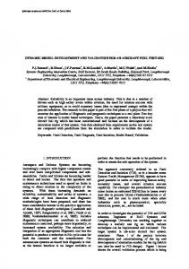
It can be seen in Fig. 11 that the contact force of the new design has a smoother curve. A statistical analysis showed that the standard deviation of the contact force was reduced to almost half the original value, being the corresponding values for the classic and the new profiles: One can see easily the range values of the contact force and the better course of the new σclassic = 8.3 N σnew = 4.5 N profile. It should kept in mind that low values for the standard deviation indicate a good dynamic behaviour of the interaction between pantograph and conductor rail. Many results instead, arrive from test and direct proof on existent infrastructure. Huang Determination of thegave maximum distance example between in supports and Chen a significative [16]: they applied a Hall-effect current probe to

Since the new a better dynamic behaviourfor than the classic one, it was wondered the first side design of the had transformer of the locomotive capture the current warring from to what degree the distance between supports could be increased for the new conductor rail without lineresults and some In this it was profile. possibleDistances to evaluate the contact obtainingthe worse in theaccelerometers. dynamic behaviour thanway, the classic of 10, and 14 m 166 H-H Huang and12 T-H Chen were simulated with the pantograph passing at a constant speed of 110 km/h. It could be shown that the quality in terms of ’contact loss’ as we can see in the figure. dynamic behaviour of the new profile with 12 to 14 m between supports is similar to the one of the classic case with 10 m. Fig. 12 shows the contact force obtained when analysing these cases.

travel speeds. Beside occurs at a speed o explained as that th the pantograph has r the vertical oscillatin value [12]

Contact Force 150

FN [N]

125 100 75 50 35

Classic - 10m 110kmh New - 12m 110kmh New - 14m 110kmh

40

45 s [m]

50

vertical oscillating 55

where v is the train sp ness of the contact w Fig. 12. Contact forces for 110 km/h conductor rail. This i As can be seen in the figure, the peaks of the contact forces do not coincide for theconductor three cases, rail in tu since the catenary supports are spaced differently (10, 12 and 14 m) and the velocity is the same. Fig. 13 pantographs are used shows the corresponding standard deviation of the contact forces. The statistical results for both profiles In addition to fin Theofpercentages contact for each speed 2.4:Fig. Percentages contact loss forofdifferent speed and are presentedFig. together, for 12 distances between supports of 10, values 12loss andof 14 m and adifferent constantkinds velocity of the current collection range of both OCSs and the equivalent probabilof catenary 110 km/h. speed, it is also neces ity for the critical standard difference among th Mandai and Shimizu did other experiments [30]. They installed 500 meters of new-profile rail OCS is installed mean rigid catenary in RTRI; by using a PS205 pantograph with 64 N of static uplift, theyand standard waveform in each tun an explanation of this transformation using a speed of evaluated that the time rate of contact loss respect the standards and that this new in Fig. 13. The mean 100 km/h. profile is better up to 200 km/h. all current collection As the speed of motion was 100 km/h, it took 3.6 s for the standard deviati the train to travel 100 m. During this period, the spark variability of the curr duration shall not exceed 25 ms, so the probability the mean level and th of contact loss is 25 ms/3.65 s = 6.95‰ for the critical the resulting power s standard at this speed. For other speeds, the equivalent Fig. 13(a), it can be probabilities of contact loss to the critical standard can

50 (km/h)

Table 3 Measurement item and standard valucs

200

Contact loss rate

ct loss rate

Maximum time length of Chapter 2.State of the Art

(20

6Omsec)

12

io

5

0

-

15

Frequency (Hz) Case of 5m span

I

100

I

I

150 200 Speed (krn/h)

I

250

Fig. 16: Appearance ofthe pan

Fig. 17: Compliance characteristics of PSZOS

Although the upward force ofthe pantograph is always fixed on this aerodynamic upward 100 equipment, an 150 200 force 150 200 Speed (km/h) on a pantograph when it is actually running. For that occurs d (km/h) reason, we measured the aerodynamic upward force of the Fig. 14: Contact loss rateevaluated with tests Fig. 2.5: Percentages of contact test pantograph by using the loss current collection test length of contact loss equipment at RTRI. Fig. 18 shows the measuring method 50 of the aerodynamic upward force, and Fig. 19 the The pantograph equipment consists on a rotating disk and a table on which it is possible measurement results of the aerodynamic upward force that 40 of the collector during the operation with the catenary. 0 the vibrations nce characteristics ofto measure works on the pantograph. "

f

5 type pantograph on the t RTRI, and measured its g. 16 shows the appearance ent. This equipment consists ntograph vibration table to an actual pantograph sliding ire. We set the upward force g. 17 shows the measurement acteristics.

E

30

Load cell

Case of 5m span

5

Freque I

100

v

2 20

.c

Fig. 17: Compliance char

10 0 100

150 Speed (km/h)

200

Fig. 15: Maximum time length of contact loss

Fig.Measurement 18: Measuring method o f an aerodynamic upward Fig. 2.6: Scheme of pantograph used for testing 5.2 of compliance characteristics offorce

pantograph

Although the upward force fixed on this equipment, an a occurs on a pantograph when it i reason, we measured the aerody test pantograph by using th equipment at RTRI. Fig. 18 sh of the aerodynamic upward measurement results of the aero works on the pantograph. Load cell

Wetheinstalled the PS205 typethepantograph the This study underlined relationship between complianceoncharacteristics of the pantograph test equipment at RTRI, and measured its pantograph and the quality of the contact. Fig. 16 shows the appearance compliance characteristics. 591 of the pantograph test equipment. This equipment consists of a rotating disk and a pantograph vibration table to a vibration test with an actual pantograph sliding 2.1.3 Systemperform Dynamic against the simulated contact wire. We set the upward force of the pantograph at 64 N.Fig. 17 shows the measurement As it concern theresults dynamic analysis of these systems, Vera, Paulin et al. [31] propose a of the compliance characteristics. study trough Finite Element Method by using Ansys, that although it is optimum for a

Fig. 18: Measuring method o f an

local analysis.

Something more similar to our idea of the model is in which Yoshizawa and Kawamura [20] propose, that is a model so schematized: 591

2.2.2 Non-contact State W lost (P(t)  0), the pantograph separate tor line. Substituting P(t) = 0 into Eqn osscilation for the deflection of the beam


13

Bow spring

(b)

The displacement of body is given as E

Figure 3. RIGID CONDUCTOR LINE PANTOGRAPH SYSTEM

Rigid conductor line

2.2.3 State Before Impact A give a definition of the contact point as

are written as follows:

y t =∆ sin ωt - d

Pan-head Pantograph-arm

2∆

y,yt

∂3 yl 1 ∂2 yl x=± : 2 = 3 =0 2 ∂x ∂x 0

Bow spring

x=0:

ρ,l,A,I,E Main spring

(a)

where τm is the time at which the mth i relationship of the velocities of the bea y(τ ˙ m ) and one of the beam after imp follows:

Fig. 2.7: Simplified

8 ∂yl ∂2 yr ∂yr ∂2 yl > > > < yl = yr , ∂x = ∂x , ∂x2 = ∂x2

k

> 3 > > : ∂ yr ∂x3

∂3 yl = ∂x3

y(0, τm ) = yt (τm

(3)

-d

Supporter

∂2 y ∂4 y + =0 ∂t 2 ∂x4

(4)

y(τ ˙ m+ ) =

Using impulse f (t), the equation flection of the beam is expressed as foll

2.2.1 Contact State At the contact state, the equations Figure 4. ANALYTICAL MODEL scheme of motion are obtained as Eqn.(1). The relationship between the ∂2 y ∂4 y displacement of the body and the beam is given as + 4 = 2 ∂t

Pan-head

ey(τ ˙ m ) + (1 +

αyl

y(0, t) = yt (t) = ε sinΩt

1

∂x

f (t)δ(x

(5)

3

Copy

in which the undulating profile of the catenary (related to the wear) is like an harmonic 2.2.2 Non-contact State When the contact force is

lost (P(t)  0), the pantograph separates from the rigid conducload on the pantograph with ! as the excitation frequency. Considering the pantograph tor line. Substituting P(t) = 0 into Eqn.(1), the equation of free osscilation for the deflection of the beam is given as follows:

like a beam on a spring, we get this equation: @ 2 q1 @ 2 q2 + 1 (b) @t2 @t2

∂2 y ∂4 y + =0 ∂t 2 ∂x4

Bow spring

2

=

(6)

(2.1)

f (x, t) The (x displacement 0)⌃ (t of body⌧is)given as Eqn.(2).

Figure 3. RIGID CONDUCTOR LINE PANTOGRAPH SYSTEM

2.2.3 State Before Impact And After Impact We

give aand definition of the contact the point asdisplacement follows: solved analytically by using the method of mapping assuming of y t =∆ sin ωt - d y,yt y(0, τm ) = yt (τm ) (7) the catenary equal to 1 and so

0

Y1 + Y2 = 1 where τm is the time at which the mth impulse was applied. (2.2) The relationship of the velocities of the beam before the mth impact -d y(τ ˙ m ) and one of the beam after impact y(τ ˙ m+ ) is written as , where Yi are the amplitudes of the modes. The solution of this ’impact problem’ follows:

k

y,yt

Phase difference 2π π

0 −π

y,yt

Phase difference Phase difference

confirms that the motion of each mode is decided by both the ˙ impact time and the y(τ ˙ m+ ) = ey(τ (8) m ) + (1 + e)y˙t (τm ) ρ,l,A,I,E π Phase difference velocity of each mode after the impact. −π

0

0 4. ANALYTICAL Figure model some dates MODEL and

Putting on the Rigid conductor line π

Using impulse f (t), the equation of oscillation for the deflection of the beam is expressed as follows:

π

2π

Center of pan-head Rigid conductor line

0

using the ’bifurcation diagram’ one can see that up ∂2 y

∂4 y

∞

+ 4 =firstly f (t)δ(x there 0) ∑ δ(t ) (9) 2 to ⌦ < 7.5 does not occur any contact loss and after this ∂tvalue, areτmperiodic ∂x -π m=1 -π

and than aperiodic.

0

0

10

RIGID CONDUCTOR LINE AND PAN-HEAD

20

Ω

Ω

20

30

30

Phase difference Phase difference

Copyright c 2008 by ASME

3

(a) 0҇Ω҇30 (a) 0҇Ω҇30 ππ

π /2

π /2 0 7.5

8 Ω

0 7.5 Figure 8.

yt (t) , y (0 , t)yt (t) , y (0 , t)

3 NUMERICAL EXAMPLES 3 NUMERICAL EXAMPLES Numerical examples are performed in order to consider the Numerical examples are performed in order to consider the relationship between the motion of the elastic model and the rigid relationship between the motion of thee elastic andthethe rigid model. (α = 4.47, ε = 0.068, = 0.8) Inmodel our study, phase difmodel. (α = 4.47, =given 0.068, e =modulo 0.8) In study, the phase differenceε is as Ωt 2π.our Figure 7 shows time histories of impact oscillation between the rigid conductor line and the ference is given as Ωt modulo 2π. Figure 7 shows time histories center of the pan-head,the andrigid also, the physical meaning of phase of impact oscillation between conductor line and the difference. center of the pan-head, also, the thebifurcation physical diagram meaning Figure 8and (a) shows on of the phase modulo difference. plane at 0  Ω  30. Numerical examples at high moving velocthe body shown in thediagram cited reference [6]. modulo Therefore, Figure 8 ities (a) of shows thearebifurcation on the numerical examples examples at at lowhigh moving velocities of the plane at 0  Ωwewill 30.show Numerical moving velocbody. Figure 8 (b) shows the bifurcation diagram on the modulo ities of the body are theFigures cited 9,reference [6]. plane at shown 7.5  Ω in  8. 10, 11, and 12 Therefore, show the time we will show histories numerical examples at low moving velocities of the of the elastic model. Fig. 8 (b), low moving diagram velocities of < 7.51) body. Figure 8 (b)Inshows thefor bifurcation onbody the (Ω modulo doesn’t9,occur shown Fig.9, and the the contact plane at 7.5 theΩcontact  8. loss Figures 10, as11, andin12 show time loss occurs at Ω = 7.51. The center of the pan-head separates histories of the elastic model. from the rigid conductor line when the displacement of the rigid In Fig. 8conductor (b), for low velocities of body (Ω 7.51) line ismoving at a minimum. This phenomenon was 7.5 y(t),yt (t)

yt (t) , y (0 , t)

Figure 9.

y (0 , t)

TIME HISTORIES OF ELASTIC MODEL AT Ω -1.5 = 7.0

10000

10002

1

10004

t

t Copyright c 2008 by ASME

Figure 11.

Rigid conductor line yt (t) Center of pan-head

Figure 14.

y (0 , t)

TIME HISTORIES OF ELASTIC MODEL AT Ω = 8.3

Rigid conductor line Center of pan-head

2 20000 20002 20004 20006 20008 20010

(t)

5

Rigid conductor line yt-1(t)

Copyright 2008 by ASME Centerc of pan-head

1

0)

TIME HISTORIES OF RIGID MODEL AT Ω

= 5.0


14

Naturally they validated the model with real experiments.

2.2

Aim of the thesis

As illustrated in the introduction, the problem of the interaction pantograph-catenary is object of study since many years; because of this thesis does not want to present something better to the others, but only wants to contribute in this field of research. Effectively, as seen before, the advantages showed by this system are relevant, so it has a lot of potentiality to explore. This work therefore wants to give an ulterior piece of the puzzle from a very general point of view; by studying this kind of system with an analytical approach in fact, allows us to analyze the behavior of the catenary, wherever it is applied in whatever conditions, avoiding computational cost related to FEM and FDM methods. This approach and his universality resends us to a more wide and general problem, one related to response of a beam under moving load, a typical case study adaptable to several real problems.

Chapter 3

Base of the model This chapter shows the theoretical scheme built for the thesis and the base of the model. This consists essentially on an infinite Euler - Bernoulli beam lumped by a periodic distribution of damper- spring supports and forced by a moving and vibrating load. This simplified model of the system is built by using the pdepe built-in function of MATLAB, a particular tool useful for partial differential equations, like the Euler-Bernoulli one. Than, in order to check the effectiveness of the results, the model is compared to an analytical solution of a similar system.

3.1

Scheme of the system

Fig. 3.1: Simplified scheme of periodically supported beam

As we can see in the figure, the rigid catenary is not so different from a beam, and the expression governing the vertical displacement zc is ⇢S

@ 2 zc @ 4 zc + EI = @t2 @x4 15

q(x, t)

(3.1)

Chapter 3.Base of the model

16

where E is the beam’s Young’s modulus, I is the second moment of inertia of the beam’s cross-sectional area, ⇢ is the the density and S is the surface of the same section of the beam. The term q represents the external factors which can be expressed as: +1 X

q(x, t) =

(k + c

n= 1

@ )zc (x @t

xn )

p˜cont (x

vt)

(3.2)

where v is the train speed p˜ is the pantograph/catenary contact force (here assumed as point load in the moving frame of reference) and xn is the position of the nth dropper; the terms k and c are referred to, respectively, the stiffness and the damping factor of the droppers. Studying this model allows us to analyze the displacement of the catenary zc useful to calculate, together with other factors, the contact force.

3.2 3.2.1

Partial Differential Equations Matlab function pdepe

The function pdepe is a built-in solver of Matlab which obtains the numerical solutions to the partial differential equation c(x, t, u, @u/@x)

where u = u(x, t),

@u =x @t

m

@ m (x f (x, t, u, @u/@x)) + s(x, t, u, @u/@x), @x

a  x  b,

m = 0, 1, 2 (3.3)

t0  t  tend the initial condition is u(x, t0 ) = u0 (x)

(3.4)

and the boundary condition at x = a and x = b are, respectively, pa (a, t, u) + qa (a, t)f (x, t, u, @u/@x) = 0

(3.5)

pb (b, t, u) + qb (b, t)f (x, t, u, @u/@x) = 0

(3.6)

The function pdepe is invoked with sol = pdepe(m, @pdeID, @pdeIC, @pdeBC, x, t,options)

(3.7)

where m = 0, 1, 2 defines the coordinate system with 0 corresponding to a Cartesian system, 1 to a cylindrical system, and 2 to a spherical system, x is a vector of values


17

for which pdepe will provide the corresponding values of u such that x(1) = a and x(end) = b, t is a vector of values for which pdepe will provide the corresponding values of u such that t(1) = t0 and t(end) = te nd, p1, p2, ... are parameters that are passed to pdeID, pdeIC, and pdeBC (they must appear in each of these functions whether or not they are used by that function), and options is set by odeset. The quantity sol(= u(t, x)) is an array sol(i, j), where i is the element number of the temporal mesh and j is the element number of the spatial mesh. Thus, sol(i, :) approximates u(t, x) at time ti at all mesh points from x(1) = a to x(end) = b. The function pde1D specifies c, f, s in Eq. (3.1) as follows: function[c, f, s] = pde1D(x, t, u, dudx) c = c(x, t, u, @u/@x)

@u ; @t

@ m f =x (x f (x, t, u, @u/@x)); @x s = s(x, t, u, @u/@x);

(3.8)

m

where dudx is the partial derivative of u with respect to x and is provided by pdepe. The function pdeIC specifies uo (x) in Eq. (3.2) as follows: functionu0 = pde1C(x) u0 = u(x, 0);

(3.9)

The function pdeBC specifies the elements pa , qa , pb , and qb , of the boundary conditions in Eq. (3.3) as follows: function[pa , qa , qb , pb ] = pdeBC(xa , ua , xb , ub , t) pa = u(a, t); qa = u(a, ˙ t);

(3.10)

pb = u(b, t); qb = u(b, ˙ t); where ua is the current solution at xa = a and ub is the current solution at xb = b, two extremes of the domain.


3.3

18

Using pdepe solver for Euler-Bernoulli beams

As seen on 3.1, the simplest model of our system is an Euler-Bernoulli beam subject to a punctual load and supported by a uniformed distribution of spring and damper (Winkler foundation).

Fig. 3.2: Beam with uniformly distributed spring-damper supports

Although this is just a simplification of the real system, it is not so easy using the pdepe built-in solver since this function doesn’t work with a 4th grade equation in space and 2nd grade in time, like our beam. This problem drove us to build a 3 unknown system like this:

8 > @ @ > 0 = @x u1 ; > @x u3 > < @ @ @ ⇢S @t u2 = EI @x @x u1 + q; > > > > : @ u3 = u2 ; @t

where q in this case represents the source term s which includes the distribution of the droppers and the input force, exactly in this way :

ku3

cu2

(x

x0 )sin(!t); terms

with the time derivation are our c and terms with space derivative are our f . Obviously, our interest is concentrated on the second equation and the main unknown is u3 related to the beam vertical displacement. In this case, we defined three naturally different boundary conditions and three initial conditions, all zeros for this preliminary phase. By using this particular solver, it easy to study the behavior both in time and in space of the beam, as we can see in the following figure, avoiding the construction of algorithms and avoiding the utilization of FEM in case of infinite elements.


19

Fig. 3.3: Shape in time and in space of the beam after an unitary input and distributed supports

In this case the input is located on the middle of the bar, naturally it is possible put it everywhere, and it also important to underline that in this phase we discretize x in ’only’ 200 points, due to high sensibility of the function to this parameter in time consuming. Naturally it is possible split the first, more general, graphic to two different ones, one shows the solution of a particular x point in the whole time domain while the other explains the behavior of the entire bar in a particular moment. 2

×10 -7

Deflection [m]

1

0

-1

-2

-3

-4

0

50

100

150

200

Time [s]

Fig. 3.4: Response in time of one point of the beam

250

Chapter 3.Base of the model 1

20

×10 -7

Deflection [m]

0.5

0

-0.5

-1

-1.5

0

20

40

60

80

100

120

140

160

180

200

Space [m]

Fig. 3.5: Response in space in a particular moment

3.4

Comparison with an analytical solution

Since we have not found any other beam model studied with the pdepe function, we need to compare the numerical solution come from our model to an analytical solution already studied for a similar system. This reference model is superstructure model without surged coupling related to a simplified model of wheel rail contact Appendix A. The following figure illustrates the system:

Fig. 3.6: 2-layers continuos support model without coupling

Assuming the subgrade as a completely rigid body, the equation of motion of the sleepers is kf (zr

zs ) + cf (z˙r

z˙s )

k b zs

cb z˙s = ms z¨s

(3.11)

where f is related to fasteners and b to ballast. Considering an harmonic solution and making zs as a function of zr , the rail vertical displacement solution is, for Re(k0 ) > 0 and Im(k0 ) > 0


H(!, x) =

21

1

( 4k03 EI

e

k0 (x ⇣)

+ ieik0 (x

⇣)

(3.12)

)

where k0 is the complex stiffness; the solution is splitted in eight different ones depending from the sign of Re(k0 ) and Im(k0 ) and from x, if it is smaller or greater than ⇣ .

3.4.1

Comparison

Defined the reference model, that is explained in detail in Appendix A, we can do the comparison. Since the analytical model gives results in terms of receptance, in the frequency domain, it was necessary to compute the Fourier’s transform to the numerical model, moving in this way from time domain to frequency one. The receptance of the beam is defined as the frequency response of the ratio between the displacement of the beam and the force applied on.

H(!, x) =

Zr (!, x) F (!)

(3.13)

where, in this case the Force is 1 Newton of an impulsive load. Naturally, in order to obtain an useful result to the discussion, it was necessary giving more frequency values in input using a for cycle. Therefore we put both the model in the same code to validate the numerical one, as we can see in the figure

Receptance

2.5

×10

-6

pdepe Analytic

2 1.5 1 0.5 0 10

Receptance

1.5

×10

20

30

40

50

60

70

80

90

100

frequency [Hz]

-6

pdepe Analytic

1 0.5 0 10

20

30

40

50

60

70

80

90

100

frequency [Hz]

Fig. 3.7: Comparison between analytical and numerical models

As the figure suggests, the results obtained are satisfactory; near the input point the numerical model has the same response to the analytical one. This means that it is


22

possible to build a model nearer to the real one, thai is the model involving discrete droppers and moving load.

y Technology Division Kokubunji-shi, Tokyo, Japan

opment of power electronics has e inverters for trains of electric plied to trains from contact lines h the pantographs mounted on necessary to adopt a contact line ontact loss within the allowable addition, high-speed railways of ucted in tunnel sections in recent

suggests that high-speed trains will increasingly run in tunnels in the future. Therefore, we determined to develop a new rigid conductor line system for high-speed operation in tunnels.

2 Features of conventional rigid conductor lines

The catenary system is now used for tunnel sections with catenary systems, rigid where high-speed trains are operated, while rigid conductor feature a simple structure and lines are for sections where train speed is lower. Fig. 1 also saves tunnel Construction shows the construction of catenary and rigid conductor line nal rigid conductor lines do not systems. When compared with the catenary system, the pantographs in current collection, rigid conductor line system features a high current capacity, collecting performance depends simple structure and easy maintenance. It also reduces the mpliance characteristics and the tunnel sectional area and saves tunnel construction costs. ct surface. This makes it difficult However, the conventional rigid conductor line system ation over 160 kmlh. cannot be used for train operation at 160 kmm or over. ductor line systems for train lh, therefore, we have developed +-- Spanlength line. Running tests have proved onductor line ensures current kmlh and is applicable In to thistrain chapter, starting from the simplified model seen in the previous section, it is gher speed due to its superb showed the construction of a model more similar to the real one where discrete supports t collection.

Chapter 4

A model with discrete supports and moving load

are included and a moving load is applied.

study is to develop and 4.1 verify rigid Discrete Supports ble high-speed operation in tunnel (a) Catenary system

of power electronics has made it for trains of electric railways. This ption of input power into trains tact loss ) are suppressed as far as y, therefore, to adopt a conductor suppress contact loss within the rters mounted on trains. Power is the contact wires on the ground s mounted on trains. Under the system, however, it is not possible ontact loss, which tends to increase I]. route length of Shinkansen lines consists of tunnel sections. This

0 02003 IEEE

Train

, i

/Rail

(Contact point)’ (b) Rigid conductor line system Fig. of 4.1: Discrete supports Fig. 1: Construction catenary and rigid conductor line system

In order to insert in the model a finite number of supports with a known stiffness instead of the uniform elastic foundation, located with a certain distance one to each other, we 587 IClT 2003 - Maribor. Slovenia referred firstly to the initial equation, without the term relative to the moving load:

23

Chapter 4.A model with discrete supports and moving load

⇢S

@ 2 zc @ 4 zc + EI 4 = 2 @t @x

+1 X

(k + c

n= 1

@ )zc (x @t

24

xn )

F (x

x0 )

(4.1)

As one can see in the formulation, the supports contribute has now an impulsive characteristic; therefore it was necessary translate it in code in the same manner we putted inside the external force in the Chapter 3, that is building a vector always zero except in the points where the supports should be on. Such a vector is used by the function where we exactly want thanks again to the function interp1. It is important to underline that while the previous chapter had only the aim to validate the code by comparing it with another model and so the structure’s data were negligible, now the values inserted in the solver influence the results so we used real data of this kind of structure and one can see them in the following table: Characteristic

Value

Cross Section Area

0.002124 m2

Inertia Moment

1.58*10 6m4

Young’s Modulus

69*109 P a

Mass Density

6.1 kg/m

Uniform Stiffness

104 N/m/m

Discrete Stiffness

2*105 N/m

Uniform Damping

102 N s/m/m

Discrete Damping

2*103 N s/m

Table 4.1: Values used for modeling with discrete supports

One again, since we didn’t have any other model developed with the same solver, it was necessary to validate this attempt. We did it comparing the results obtained from the scheme with discrete supports with data related to the one with elastic foundation, changing the value of the stiffness, that was 104 N/m2 andnowis2 ·105 N/m for each

support. The idea is that knowing the effectiveness of the Winkler foundation (vedi Cap.3), if this new model has the same response, with different value of stiffness, it is right.


1

25

×10 -5 discrete uniform

0.9 0.8

Receptance

0.7 0.6 0.5 0.4 0.3 0.2 0.1 0 10

20

30

40

50

60

70

80

90

100

Frequency [Hz]

Fig. 4.2: Receptances H(f) for uniform (blu line) and discrete supports(red line).

It is evident that we followed the same method used in the chapter three for doing the comparison between the two systems, that is to move to the frequency domain, applying the Fourier Transform, than calculating the receptance for different values of excitation frequency and than plot both the trends. The figure analyzes comparatively the two frequency response functions, and it is appreciable that in the range of frequency we are interested on, the behavior is the same. Once validated the effectiveness of the code relative to the model, we proceeded with different tests and proof, using for example other spans, other values of stiffness or damping, as it is possible to look in the following figures. As first proof, wind built a model with nine supports, one each ten meters, under an impulsive load slightly moved in the right respect to the center of the bar, since there is a support reaction. All the following model are done with an high level of refining in time and in space, taking into account a 100 meters long beam.


5

×10 -6

1

26

×10 -5

0.5 0 0 -5

-0.5 -1

-10 -1.5 -15 -50

3

×10

0

-2 -50

50

-5

1

×10

0

50

0

50

-5

0.5

2

0 1 -0.5 0

-1

-1 -50

0

50

-1.5 -50

Fig. 4.3: Behavior of the beam in four different moments of the proof.

As it possible to understand from the figure, the first graph represents the moment immediately after the point load action, and the other so on. Next figure instead shows deflections in two specific different points: 8

×10 -6

6 4

u

2 0 -2 -4 -6 -8 0

0.01

0.02

0.03

0.04

0.05

0.06

0.07

0.08

0.09

0.1

0.06

0.07

0.08

0.09

0.1

t

u

5

×10 -5

0

-5 0

0.01

0.02

0.03

0.04

0.05

t

Fig. 4.4: Time evolution for two specific points of the bar 1) where there is the support; 2) casual point.

One can see the effect of the presence of the support, relative both to the way to deflect and to the order of size; the first graph intact shows a more irregular behavior in comparison with the second one and above all the difference in amplitude since the effect of the support reduces it to 10

6.

We got another relevant result with other test; in the following two models we have, for the same length of the bar, only three supports,located approximately to - 40 meters, center and +40 meters . In the first one, we left the same value of stiffness in order to compare this model with the previous ( nine supports) and to look for the effect of the


27

changing of the span. The second test regards the stiffness, in fact we left only three supports at the same distance one to each other but we changed the value of k.

4

×10 -6

5

×10 -5

2 0 -2 0 -4 -6 -8 -10 -50

4

0

-5 -50

50

×10 -5

8

3

6

2

4

1

2

0

0

-1

-2

-2

-4

-3

-6

-4 -50

0

50

0

50

×10 -5

-8 -50

50

0

Fig. 4.5: Effect of the impulsive load in four different moments, with only three supports

6

×10 -6

4

u

2 0 -2 -4 -6 0

0.01

0.02

0.03

0.04

0.05

0.06

0.07

0.08

0.09

0.1

0.06

0.07

0.08

0.09

0.1

t 4

×10

-5

2

u

0 -2 -4 -6 -8 0

0.01

0.02

0.03

0.04

0.05

t

Fig. 4.6: Evolution in time for 1) point of the bar where is the support 2) casual point

According to this proof, we immediately can denote the different behavior of the beam, especially towards the end of the time (last graph 4.5); comparing it with the previous model with nine supports, it shows a more regular response but greater of almost one order of size. The presence of only three supports is not sufficient to assimilate the deflection, probably due to the number and due to the length of the span. In the fig.


28

4.6, one can see the similar behavior for a casual point compared to one under support, except for the order of size; this is probably related to the much distance of such a support respect to the point of application point.

1

×10 -6

2

0

1.5

-1

1

-2

0.5

-3

0

-4

-0.5

-5

-1

-6 -50

1.5

0

-1.5 -50

50

×10 -5

1.5

1

1

0.5

0.5

0

0

-0.5

-0.5

-1

-1

-1.5 -50

0

×10 -5

50

0

50

×10 -5

-1.5 -50

50

0

Fig. 4.7: Effect of the impulsive load in four different moments, with only three supports and stiffness increased

1.5

×10 -7

1

u

0.5 0 -0.5 -1 -1.5 0

0.01

0.02

0.03

0.04

0.05

0.06

0.07

0.08

0.09

0.1

0.06

0.07

0.08

0.09

0.1

t 2

×10

-5

1.5 1

u

0.5 0 -0.5 -1 -1.5 0

0.01

0.02

0.03

0.04

0.05

t

Fig. 4.8: Evolution in time for 1) point of the bar where is the support 2) casual point

Comparing these figures with the previous ones, the increasing of the value of the stiffness tends to stabilize the deflection better; moreover, according to the last figure there is a greater difference in the order of size of the response, due to bigger value of k.


4.2

29

Model with moving load

Fig. 4.9: Infinite beam on elastic (Winkler) foundation under moving load

4.2.1

Analytical approach

In order to comprehend better the system and its response it is necessary to begin explaining the analytical model on which we built our numerical simulation. Nevertheless we will analyze all the theoretical point of view in appendix Appendix B We will formulate the problem as follows: an infinite beam on an elastic foundations traversed by a constant force P moving from infinity to infinity at constant speed v. The elastic foundation is assumed to be of the Winkler type, that is the foundation reaction is directly proportional to beam deflection. On these assumption the transverse vibration of the is described by the known partial differential equation:

µ

@ 2 z(x, t) @ 4 z(x, t) @z(x, t) + EI + 2µ!b + kz(x, t) = P (x 2 4 @t @x @t

vt)

(4.2)

where !b is the circular frequency of damping and µ is the constant mass per unit length of the beam. As we told, the load is constant everywhere, as the following figure demonstrates:


30

20 15 10

Time

5 0

10

5

0

15

20

Space

Fig. 4.10: Constant load applied on the beam.

Referring to [13], let introduce a new variable:

s = (x

(4.3)

vt)

this expresses the fact that the origin of the axis move itself together with the load at speed v. By convention

=

✓

k 4EI

◆1/4

(4.4)

Since the length of the beam is infinite, it reach an almost

stationary state where it

stays practically at rest after the transit of the force. Now we can write the general equation in a new form:

4↵2

d2 z(s) d4 z(s) + ds2 ds4

8↵

where ↵ = (c/cc r) is the velocity factor and

dz(s) + 4z(s) = 8 (s) ds =(

p

(4.5)

(µ/k))!b is the damping factor.

The solution of this ODE is the steady-state response of the more general PDE seen in the third chapter. The boundary conditions are all zero. Since the solution (after the FT and IFT) is a function of a complex variable, we must know the poles and the solution is:

Chapter 4.A model with discrete supports and moving load Z

1 1

F (q)dq = ±2⇡i

n X

31

ResF (q)q=Aj

(4.6)

j=1

where Res is the residue of the function F(q) in the pole Aj . Naturally each solution depends from the poles and from the values of ↵ and , like the following examples.

Fig. 4.11: Deflection z(s) with ↵ = 0 and

Fig. 4.12: Deflection z(s) with ↵ = 1 and

=0

= 0.1


4.2.2

32

Applying to the model

As already stated, it was chosen to start with the beam on elastic foundation, uniformly supported. First of all it is important to say that we work in time domain; so we build a time vector t with a fine discretization and through a value of velocity (scalar) already defined, we set the space vector x.

t= time vector; vLoad= velocity value; x= t*vLoad; (4.7)

Evidently, each time sampling, the force goes through a certain space. For trying to obtain the same response of the theoretical and analytical model, we modified the value of S of our model; to compare the model it should be equal to 1, since we have available the results of a mono-dimensional beam. Moreover, since we can insert to the code a singular value of damping, we needed to solve this simple system :

8 > = ! ( µ )1/2 ; : b k

that is, by using the formulation of dimensionless damping and the term relative to it in the principal equation, we found the right relation between the two models. For making effectively moving the load, we wrote this in the code with a bi-diagonal matrix (instead of a vector), called by the solver using the function interp2. 2

3 61 1 0 0 07 6 7 60 1 1 0 07 4 5 0 0 1 1 0

The proof for testing the system consisted in to fix a value of

(4.8)

and to find the displace-

ments for different values of ↵, being it ↵=

v vcr

(4.9)

Chapter 4.A model with discrete supports and moving load and vcr = 2 ( the value of critic velocity. According to

33

EI 1/2 ) µ

(4.10)

= 0.1, which corresponds to c = 15, a very

small value of damping, we got this: 0.5

×10

-5

0

-0.5

u

-1

-1.5

-2

-2.5 0

50

100

150

200

250

150

200

250

150

200

250

x

2

×10 -5

1

0

u

-1

-2

-3

-4

-5 0

50

100

x

1.5

×10 -5

1

0.5

u

0

-0.5

-1

-1.5

-2 0

50

100

x

Fig. 4.13: Deflection of u (z(s)) with

= 0.1 and three different values of ↵, 0.5, 1, 2

The previous analysis was important to explain how the wave passes through the catenary together with the load, for different values of speed; this means that in each part of the beam that shape of the deflection in essentially the same, as we can see in the following image in which there are three photos of three different moments of the same bar under moving load with ↵ = 1 :

Deflection [m]

Deflection [m]

Deflection [m]

Chapter 4.A model with discrete supports and moving load 2

×10

34

-5

0 -2 -4

0 ×10 -5

50

0 ×10 -5

50

0

50

2

100

150

200

250

200

250

200

250

Space [m]

0 -2 -4 5

100

150

Space [m]

0 -5

100

150

Space [m]

Fig. 4.14: Deflection of the beam in three different moments with

=0.1 and ↵=1

Thanks to this figure one can understand better how the load moves over the beam. 4.2.2.1

Case with

=

cr

According to the same theoretical modulate which we are referring, the value of

cr

is

obtained from

=

cr

21/2 1 [ ↵2 + ((↵4 + 3)1/2 ]1/2 [s↵ + (↵4 + 3)1/2 ] ↵ 33/2

(4.11)

It is plain to see that the value of critical damping depends on the speed of the load motion. Analogously, in vibration of systems with one degree of freedom the critical damping depends on the natural frequency of the system (!b = !0 ). The dependance of critical damping on speed ↵ is graphically represented in the following figure: Andamento di Beta critico rispetto ad Alpha

7

6

Beta c

5

4

3

2

1

0

1

2

3

4

5

6

Alpha

Fig. 4.15: Dependance of critical damping

cr

on speed ↵


35

In order to apply this question to our code, we firstly calculated the values of

cr

for

each value of ↵ (0.5, 1, 2) and than evaluated the specific value of c to put in the model. At the end of simulations, we got the following results: 5

×10

-6

0

u

-5

-10

-15

-20 0

50

100

150

200

250

150

200

250

150

200

250

x

4

×10 -6

2

0

-2

u

-4

-6

-8

-10

-12

-14 0

50

100

x

1

×10 -6

0

-1

u

-2

-3

-4

-5

-6

-7 0

50

100

x

Fig. 4.16: Deflection of u (z(s)) with

Since the values of

cr

=

cr

and three different values of ↵, 0.5, 1, 2

provides values of c greater of one order to size, the vibration is

less pronounced and beam spends less time to assimilate it. For a better comprehension of the system, the following image shows the 3D model in space and time of the beam.


36

×10 -5 4

Deflection [m]

2 0 -2 -4 -6 -8 80 60 40

Space [m]

20 0

0

0.2

0.4

0.6

0.8

Time [s]

Fig. 4.17: 3D model of the beam, in time-space domain

4.3

Comparison with a FEM model

This paragraph aims to present a technique for using standard finite element packages for analyzing the dynamic response of multi-span structures under the effect of a constant moving load, in order to compare the results getting from this model with the semianalytical one presented in this thesis. To simulate the moving load, the basic principle is to apply forces and moments to all the nodes of the finite element model. Nodes near to the instantaneous force application point can than be given relatively large force values, whereas nodes away from the instantaneous force application point will have relatively small (zero) force values. When a beam is subjected to a concentrated force P, the forces on all the nodes of the beam are equal to zero except the nodes of the element s in which the load is applied. The external force vector has this form: F (t) = 000...f1s (t)f2s (t)f3s (t)f4s (t)...000

(4.12)

where fi are the equivalent nodal forces, f s (t) = [f1s (t)f2s (t)f3s (t)f4s (t)]T = P {N }

(4.13)

! " ' +(,* 4*'()$,*'5 #%('' :m1 z¨p1 + c1 (z˙p1

z˙p2 ) + k1 (zp1

z˙p1 ) + k1 (zp2 zp2 ) = F

zp1 ) = 0

(5.9)

Chapter 5.Interaction pantograph-catenary

5.3

44

Applying to the model using pdepe

Once defined theoretically the model of the pantograph and the consequent contact force acting in the contact point between the pantograph and the rigid catenary by using the Hertz theory, we are in front of a system of (essentially) three equations and three unknowns like this: 8 > > 2 4 > > ⇢S @@tz2c + EI @@xz4c = > >
m¨ zp + cz˙p + kzp = F > > > > > :f˜p/c = k lin (˜ z˜p ✏˜c ) + f0 hertz zc

Nevertheless, as seen in the third chapter, the pdepe solver does not accept as input the second derivation in time, so it was necessary to do some substitutions and get in this way a six equations system for 1DOF pantograph and an eight equations system for the 2DOF one: 0 1 0 1 0 1 0 1 DuDx(3) C B zcxx B 0 C Bzcxx C B C B C B C B C B C B⇢S C B zct C B EI ⇤ DuDx(1)C B C kc zc cc zct fp/c B C B C B C B C B1C @ B z C B C B C 0 zct @ B B C B c C C B C B C B C= B C+B C (5.10) B 0 C @t B fp/c C @x B C B C 0 k (z z ) f c p hertz p/c B C B C B C B C B C B C B C B C B m C B zpt C B C Bfp/c f0 q cp zpt kp zp C 0 @ A @ A @ A @ A 1 zp 0 zpt

As it concern the numerical values used for the simulations, we left the same values of the catenary seen in the previous chapter and, according to the pantograph we referred to the many publications and papers dealing with the theme. The following table shows the values we putted in the code for starting the simulations.


45

Element

1Dof

2Dof

Mass m1

100 kg

80 kg

Mass m2

/

50 kg

Stiffness k1

4000 N/m

4000 N/m

Stiffness k2

/

1500 N/m

Damping c1

1000 N*s/m

70 N*s/m

Damping c2

/

Roughness ✏c

10

4m

2000 N*s/m 10

4m

Static Uplift Force f0

90 N

90 N

Moving frequency of the base !q

10 Hz

10 Hz

Table 5.1: Values of pantograph and others used for simulations

According to the hertzian stiffness khertz , it was not easy to find more values because often the theoretical approach to the problem is different and also because, as said, there are no many studies about this kind of system. We chose therefore a values of khertz found more times in that publications having that same approach but regarding the traditional catenary, that is 50000 Nm

1.

In the following draw there is a complete model of train and catenary in order to understand better the coupling.


46

Tunnel

Catenary

Contact Force

Pantograph

Fig. 5.4: Interaction scheme between train and his pantograph with rigid catenary

5.3.1

Results

Firstly, we have to note one thing: since we don’t have any kind of referring about this theme, we used values that can be changed depending of the situation, both pantograph’s one and catenary; indeed, we did more tests (not appearing in this occasion) in which is


47

evident the different answer of the system depending on this. Moreover is important to say that this code requires a significant computational effort. As results to shows, we chose ones relatives to the two different pantograph and to the different velocities. We needed to change just the values of the position of the supports and the number, trying to maintain whenever the same span in term of meters and not in terms of spatial discretization. It was necessary to do this because the space vector is linked to the time one by the velocity: so increasing this, the space step was greater as well the number of supports. Let start with the result relative to the contact force that acts between catenary and

Pantograph Deflection[m] Contact Force [N]

1DOF pantograph at 20 m/s 200 150 100 50 0 60

80

100

120

140

160

180

200

220

240

260

180

200

220

240

260

x[m] 1

0.99 0.98 0.97 0.96 60

80

100

120

140

160

x [m]

Fig. 5.5: Contact force (1) and pantograph deflection (2) at 20 m/s


In the next figure one can see the same parameters when the force is moving at 50 m/s 100

50

0 150

200

250

300

350

400

450

500

550

600

650

450

500

550

600

650

x[m] 1

0.99 0.98 0.97 150

200

250

300

350

400

x [m]

Fig. 5.6: Contact force (1) and pantograph deflection (2) at 50 m/s

By applying the Fourier Transform it was possible to traspose the contact force to the frequency domain, in order to understand better the difference between the two cases


48

10 3

FT of Contact force

10 2

10 1

10

10

0

-1

0

1

2

3

4

5

6

7

8

frequency [Hz] 10 3

FT of Contact force

10 2

10 1

10

0

10 -1

0

1

2

3

4

5

6

7

8

9

frequency [Hz]

Fig. 5.7: Fourier Transform of the contact force at 20 m/s (1) and at 50 m/s

It is important to notice one important thing: due to computational problems related to the time consumption and to inability of the solver to refine more the time step, it was not possible to avoid the aliasing error and to study the behavior at high frequencies. Anyway the results got for low frequencies values are quite reliable, according to the literature. Tacking into account the pantograph system with two masses, it was done the same analysis and as it possible to watch in the following figures, it was obtained a more real result, that is a shape more conform to ones found in literature. The behavior of the contact force, for example, is less regular and it is more comparable to the contact force


calculated by Paulin et al. in [ ]. 100 50 0 -50 50

100

150

200

250

300

200

250

300

x[m] 1

0.98 0.96 0.94 0.92 50

100

150

x [m]

Fig. 5.8: Contact force (1) and pantograph deflection (2) at 20 m/s for 2DOF pantograph

Pantograph Deflection[m]

Contact Force [N]


49

300 250 200 150 100 150

200

250

300

350

400

450

500

550

600

400

450

500

550

600

x[m] 1 0.99 0.98 0.97 150

200

250

300

350

x [m]

Fig. 5.9: Contact force (1) and pantograph deflection (2) at 50 m/s for 2DOF pantograph

Also for this case it was applied the Fourier Transform to the contact force, getting the following result

FT of Contact force

10 3

10 2

10 1

10 0

10

-1

0

0.5

1

1.5

2

2.5

3

3.5

4

4.5

5

frequency [Hz] 10 3

10

2

10 1

10 0

10 -1

0

1

2

3

4

5

6

7

Fig. 5.10: Fourier Transform of the contact force at 20 m/s (1) and at 50 m/s for 2DOF pantograph

Naturally, differences are evident between the two systems, under all points of view; nevertheless the most important thing is that there is a quite stable coupling between catenary and pantograph, at least in this preliminary and approximate stadium. The goal of the thesis was, in fact, to demonstrate the feasibility of using this method for analyzing this kind of systems. The results of the simulations are shown indeed in terms


50

of the time history of the contact force acting and this, remain always with positive sign with a mean value of more than 100 N, like the results of other studies. The standard deviation,

, of the contact force is one of the main statistical variables

that characterize current collection quality. It is desirable that the standard deviation be small, since a homogeneous contact force favors the current collection process and reduces the wear. The following figure compares the standard deviation obtained for the cases studied.

Standard Deviations [N]

25

20

15

10

5

0

1DOF 20 m/s

1DOF 50 m/s

Fig. 5.11: Values of

5.3.2

2DOF 20 m/s

2DOF 50 m/s

for different systems and velocities

Simulation Times

In order to understand better how works the code we developed and the time requested to create it, it is necessary to speak about the effort in terms of computational time that the software employed to give us the results in each part of the dissertation. Naturally, we are unable to compare exactly the calculation times by using only this table because of the different time steps and different datas of the structure.The values under column T ime are to be intended respect to one second of response of the system: Case Winkler foundation and input load Comparison uniform with discrete supported (4), input load 3 discrete supports, input load 9 discrete supports, input load Winkler foundation, monodimensional beam, moving load Discrete supports, Pantograph 1Dof Discrete supports, Pantograph 2Dof

Time [s]

Time Step [s]

⇡ 45000

0,001

⇡ 240000

0.001

⇡ 6000

0.008

⇡ 1000

0.08

⇡ 125000

0.002

⇡ 1080000

0.001

⇡ 800

0.08

Table 5.2: Values of computational time for each case analyzed


51

As it is possible to note, although the system comprehensive of discrete supports and pantograph as load is the most complex, the software employed the minimum effort to comput the response: this because of the time step that is much more large than the others, since,as it was explained above, MATLAB was unable to give us the solution refining more than 0.008 the time step without modifying other parameters. As it said, this was a very big limitation of the code. The biggest value present in the table is one referred to 100 meters bar with nine equally spaced supports under the effect of the input load; in this case the time step is very tiny and the catenary in terms of structure and constrains is real. This enormous values of time consuming give us the idea of the computational effort requested to simulate real condition with fine time step.

5.4

Conclusions

A new model to study the catenary-pantograph interaction was created. Its differences are quite different from others seen in the same field; nevertheless results obtained are similar. During the development process, advanced modeling and simulations were used. Particularly a semi-analytical model as built for the catenary and a system of lumped masses was used for the pantograph schematization. A combined pantograph-catenary interaction model was set-up on the hertzian theory. Being a new one, the catenary model was validated in each its part by comparison with other models and their results. A subgrade model created for railways tracks was used to compare the receptances caused by impulsive forces and the Fryba’s theory [ ] about moving load on structures was used to evaluate the behavior of the catenary when the pantograph passes. In order to enforce our results it was built a simple FEM model in Ansys. Finally, was analyzed the kay of the interaction that is the contact force value; it was seen that the result got in our model are in agreement with ones found in literature, in terms of shape and of numerical values. Although some limitations appeared, regarding above all the time step discretization adopted in the last part, the model seems to be robust and easy to adapt to other similar systems. Maybe this sort of universality is the best result gained from this work, since it is possible to use this model in systems regarding a beam subjected to different loads, a problem always actual in our field of study.

Appendix A

Superstructure model without subgrade coupling In this appendix the analytical solution of the superstructure model presented in Section 3.4 in the assumption of no superstructure/subgrade coupling is presented. This simplified superstructure model is shown in the following figure

Fig. A.1: 2-layers continuos support model without coupling

Since the applied load is unitary, the specified problem is, of course, one of determining the Green?s function for the system. Assuming the subgrade as a completely rigid body, the equation of motion of the sleepers becomes kf (zr

zs ) + cf (z˙r

z˙s )

k b zs

cb z˙s = ms z¨s

(A.1)

ms ! 2 Zs

(A.2)

so the governing equation of the sleepers will be (kf + if )(Zr

Zs )

(kb + ib )Zs = 52

Appendix A. Superstructure Model

53

where Z is the amplitude of the response and the equation is defined in the frequency domain. In this domain the governing equation of the rail can be written as EI

@ 4 Zr @x4

⇢S! 2 Zr + (kf + i!cf )(Zr

Zs ) = Fw/r (!) (x

⇣)

(A.3)

By finding Zs from A.2 and by substituting, we get

EI

@ 4 Zr @x4

⇢S! 2 Zr + Q(!)Zr = Fw/r (!) (x

⇣)

(A.4)

where kf + i!cf kf + i!cf + kb + i!cb

Q(!) = (kf + i!cf )(1

ms ! 2

(A.5)

By the application of a Fourier Transform to A.4 and writing in this way

k 4 Z¯r

k04 Z¯r =

Fw/r ik⇣ e EI

(A.6)

where

k0 =

r 4

! 2 ⇢S Q(!) EI

(A.7)

is the complex stiffness. Therefore the rail displacement in the wavenumber-frequency domain can be defined by

Zr =

Fw/r eik⇣ EI k 4 k04

(A.8)

By applying the Fourier anti transform one can obtain the rail vertical receptance in the spatial-frequency domain Zr 1 = Fw/r 2⇡Ei

Z

1 1

e ik(x ⇣) dk k 4 k04

(A.9)

The denominator of the integrand of the equation above have four roots: k = ±k0 , ±ik0

(A.10)

If k0 is a real number, two of these four roots are real and two imaginary. For this case, it can be found the development of contour integration and the solution of this problem


54

in [ ]. But when k0 is a complex value any of the four roots are not pure real nor pure imaginary, as can be seen in figure

Fig. A.2: Poles distribution for k0 located in the first quadrant of the complex plane and integration paths

In these figures it is also presented two different integration paths that allow for a evaluation, following the contour integration technique, of the integral . Applying this approach to both paths gives the following expression Z where

R

SC

1 1

+

Z

SC

= ±2⇡i

X

Res

(A.11)

is the integration along the semicircular portion of the path and ⌃Res is

the summation of the residues of the poles inside the integration contour. The sign of P the term ±2⇡i Res is defined by the direction of rotation: positive for anti clockwise direction and negative for clockwise direction.

On one hand, the first path is used when x > ⇣ because, in this case, the integral along this semicircular path is equal to zero. On the other hand, the second path is used when x < ⇣ for the same reason. Therefore, the calculation of the integral reduces to the evaluation of the residues en- closed by the selected contour. Using Cauchy’s integral formula, to evaluate the residues in all possible cases (for the two different integration paths and for k0 in each quadrant of the complex plane) gives the rail vertical


55

displacement solution, that is defined, for Re(k0 ) > 0 and Im(k0 ) > 0 by 1 ( e k0 (x ⇣) + ieik0 (x 4k03 EI 1 H(!, x) = 3 ( ek0 (x ⇣) + ie ik0 (x 4k0 EI

⇣)

H(!, x) =

⇣)

)

x>⇣ (A.12)

)

x 0 by 1 (ek0 (x ⇣) + ieik0 (x ⇣) ) 4k03 EI 1 H(!, x) = 3 (e k0 (x ⇣) + ie ik0 (x ⇣) ) 4k0 EI H(!, x) =

x>⇣ (A.13) x⇣

)

x 0 and Im(k0 ) < 0 by 1

H(!, x) =

( 4k03 EI

e

H(!, x) =

1 ( ek0 (x 3 4k0 EI

⇣)

ik0 (x ⇣)

ieik0 (x

⇣)

)

x>⇣ (A.15)

)

x

Development for an efficient model for pantograph ...

Development for an efficient model for pantograph ...

Suggest Documents

An Efficient Objective Quality Model for Agile Application Development

an efficient fair queuing model for data

An efficient model-based methodology for developing

An Efficient Component Model for the Construction

An efficient tension-stiffening model for nonlinear

An Efficient Computational Model for Premixed ...

An Efficient Framework for Hydrologic Model ...

An efficient descriptor model for designing materials for solar cells

Use of Hoeken's and Pantograph Mechanisms for

An efficient model for dimensioning an ATA-based ...

Development of an object model for automated

An Evaluation Model for Social Development Environments

SMME MODEL FOR ECONOMIC DEVELOPMENT AN ...

DEVELOPMENT OF AN INTEGRATED MODEL FOR

DYNAMIC MODEL DEVELOPMENT AND VALIDATION FOR AN ...

Development of an empowerment model for burnout

Model-based Toolchain for the Efficient Development of ... - Google Sites

Automatic Development of an Abstract Context Model for an ... - PRIMA

An Efficient Multibody Dynamics Model for Internal Combustion ...

An Efficient Cost Model for Optimization of Nearest Neighbor Search ...

An Efficient Architecture Model for Systematic Design of Application ...

Developing an efficient model for evaluating WWW Search Engines

An Abacus Turn Model for Time/Space-Efficient ...

An efficient chloride ingress model for long-term ...