GAS-PARTICLES MULTI-FLUID SYSTEMS USING KINETIC THEORY ... An Eulerian multiphase gas-solid solver with kinetic theory closure has been developed and ...... Journal of Applied Mathematics and Physics, 31:483â493, 1980. Park I.
Mecánica Computacional Vol XXXIII, págs. 473-497 (artículo completo) Graciela Bertolino, Mariano Cantero, Mario Storti y Federico Teruel (Eds.) San Carlos de Bariloche, 23-26 Setiembre 2014
DEVELOPMENT OF A CONSERVATIVE NUMERICAL SOLVER FOR GAS-PARTICLES MULTI-FLUID SYSTEMS USING KINETIC THEORY OF GRANULAR FLOW Cesar Veniera , Santiago Marquez Damiana , Damian Ramajoa and Norberto Nigroa a Centro
de Investigacion de Metodos Computacionales (CIMEC) UNL-CONICET, S3000GLN Santa Fe, Argentina
Keywords: CFD, Multiphase Flow, Fluidized Bed, Drag Model, Kinetic Theory of Granular Flow Abstract. An Eulerian multiphase gas-solid solver with kinetic theory closure has been developed and implemented on the open-source code OpenFOAM R . In order to increase the accuracy of the model, a fully conservative form of the momentum equations has been adopted, keeping the phase fraction in both space and time derivatives. The enforcement of the packing limit has been addressed by an implicit treatment of the particle pressure contribution on the phase continuity equation, and a semi-implicit treatment of the drag term on the momentum equations has been used to construct the face fluxes needed by the algorithm. The solver has been tested against standard multiphase cases, where analytical or numerical solutions are available for comparison.
Copyright © 2014 Asociación Argentina de Mecánica Computacional http://www.amcaonline.org.ar
474
1
C. VENIER, S. MARQUEZ DAMIAN, D. RAMAJO, N. NIGRO
INTRODUCTION
Fuidized bed regimes of multiphase solid-gas flows may be found in many industrial applications, from energy production reactors to grain drying systems. One of such applications is the riser of a Fluid Catalytic Cracking (FCC) reactor, in which the interaction between particles affects the global efficiency of the system. A proper understanding of such systems is critical to predict results and designing units. In this context, a CFD approach becomes an inexpensive tool and may complement experimental techniques for the study of large multiphase systems behavior (Min et al., 2010; Almuttahar and Taghipour, 2008). One of the many issues in developing a two-phase solid-gas flow solver is the numerical effort involved in solving a system with a large number of particles. The Eulerian approach considers a solid phase with no particle tracking and a fluid-like behavior, thus having a set of mass and momentum balance equations for the solid phase. This technique presents the drawback of lacking of a proper physical definition for the particles stress tensor, which may be remedied with the introduction of the granular energy concept and the Kinetic Theory of Granular Flow (Gidaspow (1994), Lun et al. (1984)) to provide a mathematical closure. Another subject arises when a large gradient transport problem is being solved numerically. The issue is based on the fact that different solutions may be found when the non-conservative formulation of the momentum equations is adopted. This topic has been studied by Staedtke (2006) and Leveque (2002), who showed that a conservative formulation leads to more accurate solutions in these kind of problems. In this work, we developed a two-phase solid-gas solver on the OpenFOAM R (Weller et al., 1998) platform, based on the standard twoPhaseEulerFoam solver with the implementation of the MULES limiter, the kinetic and frictional theory models and the conservative treatment of the momentum equations based on the study of Passalacqua and Fox (2011). As a reminder of the present work, the next sections are organized as follows. In Section 2, the theoretical framework of the two-phase solid-gas flow system with kinetic and frictional theory closures is presented. Section 3 describes the numerical aspects of the code implementation. Finally, in Section 4, a series of benchmark problems are simulated in order to test the performance of our solver, by comparing against both analytical and numerical solutions. 2
MULTIPHASE MODEL
2.1
Governing Equations
The Eulerian model for multiphase systems is basedP on the fact that both phases are treated as interpenetrating continua (Gidaspow, 1994), where i αi = 1 must be verified. The mass and momentum equations for the solid phase are: ∂ (αs ρs ) + ∇· (αs ρs us ) = 0 ∂t
(1)
and ∂ (αs ρs us ) + ∇· (αs ρs us us ) = ∇· (αs τ s ) − αs ∇p − ∇ps + αs ρs g + Ksg (ug − us ) ∂t where 2 τ s = µs [∇us + ∇uTs ] + (λs − µs )(∇· us )I 3
(2)
(3)
Copyright © 2014 Asociación Argentina de Mecánica Computacional http://www.amcaonline.org.ar
Mecánica Computacional Vol XXXIII, págs. 473-497 (2014)
475
While for the gas phase are: ∂ (αg ρg ) + ∇· (αg ρg ug ) = 0 ∂t
(4)
and ∂ (αg ρg ug ) + ∇· (αg ρg ug ug ) = ∇· (αg τ g ) − αg ∇p + αg ρg g + Ksg (us − ug ) ∂t where
(5)
2 (6) τ g = µg [∇ug + ∇uTg ] − µg (∇· ug )I 3 In order to solve the governing equations, several unknown terms require modeling. These models are known as closure laws. For the present study, the lift and virtual mass effects have been neglected and the phases are coupled through the drag force term. For example, a general form for the drag coefficient may be modelled as (Schiller and Naumann, 1933): Ksg = 0.75
Cd αs αg ρg |ug − us | dp
(7)
where the drag force increases with the square of the relative velocity module between phases. For a list of the available models for the drag coefficients in OpenFOAM R see the Appendix. 2.2
KTGF and Frictional Models
Due to the need of a mathematical model for the solid phase global stress tensor (which lacks of a proper definition when the solid phase is treated as a fluid), different flow regimes need to be taken into account: • If the particles are present in a dilute state, then the grains translate freely. This regime is known as Kinetic Regime. • If the particles are present in a higher concentration, then, in addition to the previous effects, the grains may collide with each other. This regime is known as Collisional Regime. • If the particles are present in a very high concentration, the grains not only collide instantly, but there is friction and rubbing between particles. This regime is known as Frictional Regime. The Kinetic Theory of Granular Flow (Gidaspow, 1994; Lun et al., 1984) provides a set of mathematical models to contemplate the effects of the Kinetic and Collisional regimes. This theory introduces the concept of granular temperature (θs ) as a primitive variable from which the solid phase stress tensor may be modeled. A granular energy may be defined as a specific kinetic energy due to the granular random motion of the particles: 1 3 Esg = |c′ |2 = θs 2 2 Copyright © 2014 Asociación Argentina de Mecánica Computacional http://www.amcaonline.org.ar
(8)
476
C. VENIER, S. MARQUEZ DAMIAN, D. RAMAJO, N. NIGRO
where c′ represents the velocity of the chaotic motion of the grains. The microscopic balance equation of the granular energy is given by Eq. (9): i 3h ∂ (αs ρs θs ) + ∇· (αs ρs us θs ) = (−ps I + τ s ) : ∇us + ∇· (κs ∇θs ) − γs + Jvis 2 ∂t
(9)
The following models are based on the solution of the previous equation (see Van Wachem (2000)):
γs =
3ρs αs2 g0 (1
−
e2p )θs
4 dp
r
θs − ∇· us π
!
� √ 15 √ 25 πg0 2αs2 g0 (1 + ep ) 9√ 2 √ κ s = ρs d p θ παs g0 (1 + ep ) + παs + + 16 16 64(1 + ep ) π Jvis = −3Ksg θs √
�
On the other hand, when the solid volume fraction reaches a critical high value (usually αs ≃ 0.6), the contact between particles are no longer given by binary collisions but from the effects of rubbing and friction with each other. Therefore, the assumption of instant contact, used by the kinetic theory, is no longer valid and frictional stress models must be employed. Hence, the modeling of the solid stress tensor switches between theories when this critical solid volume fraction is reached (known as αs,min ). This implies different contributions for each regime, in order to define µs and ps : µs = µs,col + µs,kin + µs,f ric
(10)
To illustrate the variables involved, we present some of the models that may be used to calculate the solid phase viscosity (Gidaspow, 1994; Johnson and Jackson, 1987): √ �2 � 4 10ρs dp θs π µs,kin = 1 + (1 − ep )αs g0 96g0 (1 + ep ) 5 � �1/2 4 θs µs,col = ρs αs2 dp g0 (1 − ep ) 5 π −1/2
µs,f ric = 0.5ps I2D sin(φ)
� �1/2 θs 4 2 λs = ρs αs dp g0 (1 − ep ) 3 π Analogous to the particle viscosity, the particle pressure includes a kinetic, collisional and frictional contribution (Lun et al., 1984; Johnson and Jackson, 1987): ps = ps,col + ps,kin + ps,f ric
(11)
where ps,kin = ρs αs θs ps,col = 2ρs αs2 g0 (1 − ep )θs (αs − αs,min )η ps,f ric = F r (αs,max − αs )P Copyright © 2014 Asociación Argentina de Mecánica Computacional http://www.amcaonline.org.ar
Mecánica Computacional Vol XXXIII, págs. 473-497 (2014)
477
The radial distribution may be defined as (Carnahan and Starling, 1969): g0 = 3
3αs αs2 1 + + (1 − αs ) 2(1 − αs )2 2(1 − αs )3
(12)
NUMERICAL TREATMENT
The equations are solved using the Finite Volume Method with both phases treated under an incompressible flow hypothesis (Ferziger and Peric, 2002; Jasak, 1996) and the PIMPLE algorithm for the pressure-velocity coupling (Issa, 1985; Caretto et al., 1973). Hence, the continuum mass and momentum equations become: ∂αs + ∇· (αs us ) = 0 ∂t ∂ 1 αs 1 Ksg (αs us ) + ∇· (αs us us ) = ∇· (αs τ s ) − ∇p − ∇ps + αs g + (ug − us ) ∂t ρs ρs ρs ρs
3.1
(13)
(14)
∂αg + ∇· (αg ug ) = 0 ∂t
(15)
1 αg Ksg ∂ (αg ug ) + ∇· (αg ug ug ) = ∇· (αg τ g ) − ∇p + αg g + (us − ug ) ∂t ρg ρg ρg
(16)
Momentum Equation
One of the main issues of solving the equations presented in Eq. (13), (14), (15) and (16) is that we will come to the difficulty of having the volume fraction in all the terms, thus having a null equation when one of the phases is not present. A non-conservative formulation, as presented by Weller (2002), may solve this problem by expanding the derivative of the products with αs , dividing all by αs and isolating the terms in which the phase fraction remains. These terms could be easily treated to avoid singularities, nevertheless, the discretized equation derived from this formulation may not provide an accurate solution when solving shock-waves. This behavior is explained by Leveque (2002) and Staedtke (2006), and will be discussed later on. In this work, we will adopt the conservative formulation to increase the robustness of our solver and deal with the phase fraction tending to zero, by avoiding the solution in those cells where the phase fraction becomes smaller than a certain “cutoff” value. The semi-discrete form of the momentum equations are: As us = Hs −
αs 1 Ksg ∇p − ∇ps + αs g + (ug − us ) ρs ρs ρs
(17)
αg Ksg ∇p + αg g + (us − ug ) (18) ρg ρg Where Hi includes the off-diagonal contributions and Ai condensates the diagonal coefficients. Now we may define the coefficients: Ag ug = Hg −
ζs =
1 As +
Ksg ρs
Copyright © 2014 Asociación Argentina de Mecánica Computacional http://www.amcaonline.org.ar
(19)
478
C. VENIER, S. MARQUEZ DAMIAN, D. RAMAJO, N. NIGRO
ζg =
1 Ag +
Ksg ρg
(20)
and arrive to the following expressions for the phase velocities: � � Ksg αs 1 us = ζs Hs + Hg − ∇p − ∇ps + αs g ρs ρs ρs � � Ksg αg ug = ζg Hg + Hs − ∇p + αg g ρg ρg
(21) (22)
Therefore, the face velocities fluxes are computed as:
ϕs =
X f
(
ζs,f
�
) �α �1 � � � Ksg s Hs + Hg + αs g · S − ζs,f ∇p · S − ζs,f ∇ps · S ρs ρs ρs f f f
ϕg =
X f
(
ζg,f
�
) � � �α Ksg g Hg + Hs + αg g · S − ζg,f ∇p · S ρg ρg f f
(23)
(24)
where S represents the face-normal vector for each cell face. 3.2
Continuity Equation P Since i αi = 1 must be verified locally at each time step, we may solve one phase continuity equation and derive the volume fraction of the remaining phase by applying the latter condition. Thus, solving the continuity equation for the solid phase will allow us to introduce the particle pressure flux contribution implicitly to enforce the solid packing limit (see Passalacqua and Fox (2011)). ∂αs + ∇· (αs us ) = 0 ∂t This equation can be rewritten in a semi-discrete form as: ∂αs X + αs,f ϕs = 0 ∂t f
(25)
(26)
Leaving out the particle pressure flux contribution: � ∂p � 1 s ζs,f |S|∇αs (27) ρs ∂αs f Here, the definition of ϕs is taken from Eq. (23). The bounding of the phase fraction between zero and one is achieved using the MULES limiter (see Marquez Damian (2013)). Then, by defining the mixture and relative fluxes as: ϕ′s = ϕs +
ϕ = αg,f ϕg + αs,f ϕs
(28)
ϕr,s = ϕs − ϕg
(29)
Copyright © 2014 Asociación Argentina de Mecánica Computacional http://www.amcaonline.org.ar
479
Mecánica Computacional Vol XXXIII, págs. 473-497 (2014)
where: � ∂p � 1 s αs,f ζs,f |S|∇αs ρs ∂αs f � ∂p � 1 s ′ |S|∇αs ϕr,s = ϕr,s + ζs,f ρs ∂αs f We arrive to the final semi-discrete form of the phase continuity equation: ϕ′ = ϕ +
(30) (31)
� ∂p � X ∂αs X 1 s + |S|∇αs = 0 (αs ϕ′ )f + (αs αg ϕ′r,s )f − αs,f ζs,f ∂t ρ ∂α s s f f f 3.3
(32)
Pressure Equation
If we sum up both solid and gas phase continuity equations, we obtain: ∇· ϕ = 0
(33)
where ϕ was defined in Eq. (28). Now, if we apply divergence on the phase velocity fluxes in each term of Eq. (23) and (24) and considering Eq. (33), we may arrive to the following expression for the pressure equation: �α � i o �α � nh s g ∇· αs,f ζs,f (∇p· S) = ∇· ϕ0 + αg,f ζg,f (34) ρs f ρg f where:
ϕ0 = αs,f ϕ0s + αg,f ϕ0g ϕ0s =
(
(35) h1
Ksg Hg + αs g · S − ζs,f ∇ps · S ρs ρs f f f ) ( i h X K sg Hs + α g g · S ϕ0g = ζg,f Hg + ρ f g f
X
h
ζs,f Hs +
i
i
)
(36)
(37)
Finally, solving Eq. (34) we can correct the phase velocity fluxes by including (∇p· S) on Eq. (23). 3.4
On the conservative treatment of the momentum equations
One major difference between the standard two-phase solvers that are available on the OpenFOAM R distribution and the one developed in this work, is the conservative treatment of the momentum equations. This concept refers to the way that both αi and ui are operating in the advective and transient terms of the discrete momentum equation. We may reformulate Eqs. (14) and (16) as follows: ∂ (αs ui ) + ∇· (αi ui ui ) = Ri ∂t where Ri represents all the terms on the right- hand-side of Eqs. (14) and (16).
Copyright © 2014 Asociación Argentina de Mecánica Computacional http://www.amcaonline.org.ar
(38)
480
C. VENIER, S. MARQUEZ DAMIAN, D. RAMAJO, N. NIGRO
Now the derivatives on both terms on the left-hand-side of Eq. (38) may be expressed as: αi
∂αi ∂ (ui ) + (αi ui )· ∇ui + ui + ui ∇· (αi ui ) = Ri ∂t ∂t
(39)
Here the last two terms of the left-hand-side may be neglected considering the continuity equations form Eqs. (13) and (15). Thus having: αi
∂ (ui ) + (αi ui )· ∇ui = Ri ∂t
(40)
which is the non-conservative form of the momentum equations and the one implemented in several two-phase solvers on OpenFOAM R . This formulation is consistent with the conservative form (Eq. (38)), being both equal in the continuum. Nonetheless, the discretization practice of Eq. (40) may lead to inaccurate results under certain flow conditions. Staedtke (2006) and Leveque (2002) show that the numerical integration of the non-conservative form of the momentum equations may cause a misbehavior in the solution for high gradient transport problems, such as shock-waves and density currents. Moreover, Park et al. (2009) proposed some conceptual problems to evaluate the solution of a non-conservative formulation against a semi-conservative form, where only the advective term has been treated as in Eq. (38). The solutions shows more accurate results for the semiconservative form in cases such as a phase separation problem, where the front velocity of each phase may be found analytically under a quasi-steady state assumption (Staedtke, 2006). Two-phase flow problems, specially gas-solid flows, usually involves large gradients transport due to the high density difference between phases, therefore we developed our two-phase solver based on the numerical integration of the conservative form of the phase momentum equations (Eq. (38)). 3.5
The PIMPLE algorithm
The algorithm used to couple the pressure field is a combination of PISO (Issa, 1985) and SIMPLE (Caretto et al., 1973), called PIMPLE, which allows to introduce under-relaxation factors to enforce the convergence of the iterative procedure and outer iterations in order to improve the coupling between momentum and mass conservation equations. The sequence consists of the following steps: 1. Start the continuity equation loop a. Solve Eq. (32) without the particle pressure contribution, using MULES limiter. ∂ps and correct the continuity equation to re-obtain αs . If the kinetic b. Calculate ∂αs theory is used, solve the granular temperature θs (Eq. (9)) in order to obtain the kinetic particle pressure ps (Eq. (11)) c. Calculate αg = (1 − αs )
d. Iterate from a. until a convergence criterion is reached
2. Calculate the drag coefficient Ksg Copyright © 2014 Asociación Argentina de Mecánica Computacional http://www.amcaonline.org.ar
Mecánica Computacional Vol XXXIII, págs. 473-497 (2014)
481
3. Update the momentum equation coefficients 4. Solve the predicted velocity from the phase momentum equation with the previously stored pressure 5. Start the pressure equation loop a. Obtain the interpolated values of the phase fraction αi and momentum coefficients Hi and ζi on the cell faces b. Construct the partial phase fluxes given by Eq. (36) and (37) c. Construct the pressure flux contribution coefficient d. Solve the pressure equation and correct for non-orthogonal meshes e. Correct the face fluxes with the pressure flux contribution f. Correct the cell centered phase velocities 6. Iterate from 1. until a convergence criterion is reached 4
TEST CASES
In this section, we present a series of test cases to validate our two-phase solver. In order to do so, we started studying a one-dimensional water faucet problem, in which a two-fluid mixture flow descends down a tube and a phase segregation wave propagates through it. This type of problem allow us to test the performance of the interpolation schemes in large gradients transport problems. Next, we present a horizontal transport of particles problem, in which a momentum transfer between phases takes place. Here the performance of the drag numerical implementation is tested under different mesh refinements and different particles volume fraction. Then, we present results for a solid settling suspension problem, with and without a packing limit. This test allow us to study the behavior of the kinetic theory numerical implementation and the solver performance under more critical conditions, such as reaching the packing limit and near-zero phase fraction. Finally, we present a more practical problem with industrial applications: a fluidized bed. In this test, we evaluate our solver performance in all general aspects and the solutions are compared against the ones from authors using the OpenFOAM R platform. 4.1
Water Faucet
The Water Faucet problem (Ransom and Mousseau, 1991) has been widely studied by several authors (Corzo et al. (2012), Nourgaliev et al. (2003)) over the years and established as a numerical benchmark to test the performance of two-phase flow solvers. This test consists of a vertical tube of 12 m length and 1 m diameter. The tube is initially filled with an air-water homogeneous mixture with a liquid phase fraction αl0 = 0.8 and density ratio ρl /ρg = 1000. The initial and boundary conditions are summarized in Table 1 Due to the gravity acceleration and mass conservation, the liquid vein diameter decreases and a phase fraction discontinuity propagates downward. Here the momentum transfer term is negligible and the dominant effect is the gravity force.
Copyright © 2014 Asociación Argentina de Mecánica Computacional http://www.amcaonline.org.ar
482
C. VENIER, S. MARQUEZ DAMIAN, D. RAMAJO, N. NIGRO
intlet
Field αl0 αl,inlet u0l (m/s) ul,inlet (m/s) u0g (m/s) ug,inlet (m/s)
g
initial state
steady state
outlet
Figure 1: Water Faucet test case scheme
Value 0.8 0.8 10.0 10.0 0.0 0.0
Table 1: Initial and boundary conditions
The analytical solution for αg is given by: gt2 αl0 u0l 0 , if y ≤ u t + αg (y, t) = 1 − p l 2 2gy + (u0l )2
(41)
The following results have been obtained with a time step of 1 × 10⁻⁴ s and 240 uniform square cells for the space discretization on the vertical direction. The simulations were performed using 3 PIMPLE iterations. In Figure 2, different advection schemes are presented to compare with the analytical solution for the gas volume fraction wave propagation at t = 0.5 s. 0.5 Analytical Full Upwind Central Difference Linear Upwind van Leer
0.45
Air Volume Fraction
0.4 0.35 0.3 0.25 0.2 0.15 0
2
4
6 x (m)
8
10
12
Figure 2: Analytical and numerical solution at t = 0.5 s with different advection schemes
Copyright © 2014 Asociación Argentina de Mecánica Computacional http://www.amcaonline.org.ar
Mecánica Computacional Vol XXXIII, págs. 473-497 (2014)
483
The results show that the van Leer scheme produces the highest balance between accuracy and stability, where the oscillatory behavior, seen with the Central Difference method, is mostly suppressed and a sharp wave-front is achieved to capture the high gradients near the discontinuity. 4.2
Horizontal Transport of Particles
This problem consists of a one-dimensional transport of solid particles diluted in an air flow with a density relation of ρs /ρg = 2000 and a particle radius of rp = 1 mm. The inlet velocity of the air is higher than the inlet velocity of the particles, so the particles are accelerated due to the momentum transfer and reach an equilibrium velocity given by: g s usinlet uginlet + αinlet Ueq = αinlet
inlet condition velocity fixed
(42)
outlet condition pressure fixed P
Ug, Us
Figure 3: Horizontal transport test case
Eq. (43) was deducted by (Morsi and Alexander, 1972) under the assumption of having a constant drag coefficient for the momentum transfer modeling, and a solid volume fraction tending to zero. 3 ρg C D Ug,inlet Ug,inlet = x + ln(Ug,inlet − Us,inlet ) + Ug,inlet − us 4 ρs r p Ug,inlet − Us,inlet (43) The following results are obtained for a time step of 1 × 10⁻³ s and for different space refinements. In Figure 4, the solid volume fraction distribution for different mesh refinements may be noted. ln(Ug,inlet − us ) +
Copyright © 2014 Asociación Argentina de Mecánica Computacional http://www.amcaonline.org.ar
484
C. VENIER, S. MARQUEZ DAMIAN, D. RAMAJO, N. NIGRO
3.5
Solid particles velocity [m/s]
3
2.5
2 Analytical solution 50 Cells 100 Cells 500 Cells
1.5
1 0
2
4
6
8
10
x [m]
Figure 4: Solid particles velocity for different number of cells
In Figure 5, results for different solid volume fraction are presented, and a range of applicability of Eq. (43) may be observed. Corzo et al. (2012) and Moukalled and Darwish (2002) also provided numerical solutions but with a non-conservative formulation of the momentum equation.
3.5
Solid particles velocity [m/s]
3
2.5
2 Analytical solution Solid Vol. Frac. 0.00001 Solid Vol. Frac. 0.01 Solid Vol. Frac. 0.1
1.5
1 0
2
4
6
8
10
x [m]
Figure 5: Solid particles velocity for different volume fractions
Copyright © 2014 Asociación Argentina de Mecánica Computacional http://www.amcaonline.org.ar
Mecánica Computacional Vol XXXIII, págs. 473-497 (2014)
4.3
485
Settling Suspension
A one-dimensional two-phase liquid-gas settling suspension problem was simulated in a 1 m vertical tube using an 80-cells grid. The initial condition of the volume fraction of the disperse phase is αl0 = 0.5 distributed uniformly over the domain. A counter-current flow is developed under the effects of gravity due to the different phase densities, and the system reaches a steady state when the dense phase settles completely on the bottom of the tube. pure gas
U gas
mixture
g
L U liq
pure liquid
Figure 6: Settling suspension test case
An analytical solution for each phase velocity is deducted by Staedtke (2006) under the assumption of a quasi-steady state and neglecting momentum flux terms and virtual mass forces (Eq. (44)). ∆U = Ug − Ul = Where:
h 8(ρ − ρ )r g i1/2 l g p 3CD ρm
Ug = αl ∆U Ul = −αg ∆U
(44)
(45)
The gas phase front velocity computed with Eq. (45) for this case is Ug = 0.122 m/s which is in agreement with the front velocity obtained numerically (see Figure 7 and 8).
Copyright © 2014 Asociación Argentina de Mecánica Computacional http://www.amcaonline.org.ar
486
C. VENIER, S. MARQUEZ DAMIAN, D. RAMAJO, N. NIGRO
0,6 Numerical solution at t=2.5s Analytical solution at t=2.5s Numerical solution at t=4s Analytical solution at t=4s
Gas Volume Fraction
0,5
0,4
0,3
0,2
0,1
0
0
0,1
0,2
0,3
0,4
0,5
y [m]
Figure 7: Numerical and analytical solutions for the phase segregation at different times frames
Gas phase velocity [m/s] and volume fraction
0,6 Gas phase front velocity Gas volume fraction
0,5 0,4 0,3 0,2 0,1 0 0,1
0
0,1
0,2
0,3
0,4
0,5
y [m]
Figure 8: Gas phase front velocity and volume fraction at t = 2.5 s
The agreement between the analytical and the numerical solutions in terms of the velocity fields (see Figure 7) was expected due to the use of a conservative formulation. 4.4
Packed Settling
Simulations of a settling solid-gas mixture have been carried out to test the numerical performance of the granular theory implementation. The test case is similar to the one studied previously, with the difference that now the disperse phase consists of solid particles. This phase has an uniform initial distribution of αs0 = 0.3 over a one-dimensional domain of L = 0.3 m. Copyright © 2014 Asociación Argentina de Mecánica Computacional http://www.amcaonline.org.ar
487
Mecánica Computacional Vol XXXIII, págs. 473-497 (2014)
Here we used the Schiller-Naumann model (Schiller and Naumann, 1933) for the drag coefficient and the full granular balance equation (see Eq. (9)) to compute θs . The nearpacking limit region is governed by the frictional regime models where the maximum packing is αs,max = 0.65, while the most diluted regime (for αs < 0.55) is governed by the kinetic theory models. A first order implicit time scheme was used with ∆t = 1 × 10⁻⁴ s, while a uniform 150-cells grid was used for the space discretization and a Central Difference interpolation scheme for the advective terms. 0.7 t = 0.1s t = 0.15s t = 0.2s t = 0.3s
Solid Volume Fraction
0.6 0.5 0.4 0.3 0.2 0.1 0 0
0.05
0.1
0.15 y [m]
0.2
0.25
0.3
Figure 9: Solid volume fraction evolution
600 t = 0.1s t = 0.15s t = 0.2s t = 0.3s
500
Pressure [Pa]
400
300
200
100
0 0
0.05
0.1
0.15 y [m]
0.2
0.25
0.3
Figure 10: Pressure evolution In Figure 9, the phase segregation transient state may be observed, where a constant packing limit is reached at αs ≃ 0.61. Two sharp wave-fronts propagate at counter-current and meet, Copyright © 2014 Asociación Argentina de Mecánica Computacional http://www.amcaonline.org.ar
488
C. VENIER, S. MARQUEZ DAMIAN, D. RAMAJO, N. NIGRO
reaching a completely settled steady state at t = 0.3 s. The pressure profile evolution of the mixed phases is shown in Figure 10. Constant pressure gradients at both settled regions may be observed, and a sharp solid-gas interface is achieved at the steady state, which is consistent with the expected physical behavior. 4.5
Fluidized Bed
A fluidized bed problem was simulated to evaluate the performance of the solver on a more practical case, where all the aspects studied in the previous cases may be tested (such as the near-packing condition). The numerical and physical parameters used in this case are detailed on Table 2: Group
Description Value Gas density 1.4 Kg/m3 Gas viscosity 1.8 × 10− 5 Pa.s Phase properties Particle density 2000 Kg/m3 Particle diameter 350 × 10−6 m Width 0.138 m Height 1m Geometry Bed initial height 0.2 m Grid 14 × 100 (structured squares) Timestep 1.0 × 10⁻⁴ s Overall simulation time 30.0 s Numerical method Time discretization Second order, implicit Momentum discretization Central difference Volume fraction discretization TVD limited linear Drag Syamlal-O’Brien Particle pressure Lun Kinetic viscosity Gidaspow Drag and Radial distribution Carnahan-Starling KTGF Thermal conductivity Gidaspow models Frictional stress Johnson-Jackson Restitution coefficient 0.9 Wall solid velocity slip Vertical inlet gas velocity 0.54 m/s Initial and 0 Pa boundary conditions Outlet pressure Initial bed packing 0.58 Table 2: General parameters The results of solid volume fraction and pressure drop (averaged between 5 s and 30 s) at different sections are shown in Figures 11, 12 and 13. The results are compared against the ones obtained by Passalacqua and Fox (2011) and the ones obtained with a non-conservative formulation (Venier et al., 2013).
Copyright © 2014 Asociación Argentina de Mecánica Computacional http://www.amcaonline.org.ar
489
Mecánica Computacional Vol XXXIII, págs. 473-497 (2014)
0.7
Solid Volume Fraction
0.6
0.5
0.4
0.3
0.2
Non-conservative formulation Passalacqua et al. This work
0.1
0 0
0.02
0.04
0.06
0.08
0.1
0.12
x [m]
Figure 11: Time-averaged solid volume fraction distribution at y = 0.16m
1
Non-conservative formulation Passalacqua et al. This work
0.8
y [m]
0.6
0.4
0.2
0 0
0.1
0.2
0.3
0.4
0.5
Solid Volume Fraction
Figure 12: Time-averaged solid volume fraction along the vertical direction
Copyright © 2014 Asociación Argentina de Mecánica Computacional http://www.amcaonline.org.ar
490
C. VENIER, S. MARQUEZ DAMIAN, D. RAMAJO, N. NIGRO
3000
Non-conservative formulation Passalacqua et al. This work
2500
Pressure [Pa]
2000
1500
1000
500
0 0
0.2
0.4
0.6
0.8
1
y [m]
Figure 13: Time-averaged pressure drop along the vertical direction The results show a good agreement with the ones obtained by Passalacqua and Fox (2011) with slight differences in the time-averaged solid fraction near the walls (see Figure 11). This may be due to the boundary conditions used for the solid phase velocity (since Passalacqua and Fox (2011) use a partial slip condition). Nonetheless, the field profiles for the pressure and the solid fraction show more accurate results when using a conservative formulation, against the non-conservative one. 5
CONCLUSIONS
In this work, a two-phase flow solver with kinetic theory for granular flows capability was developed using the OpenFOAM R platform. In contrast with the available solvers, a conservative formulation for the momentum equation was implemented to improve the robustness and accuracy of our code. The program was tested against a series of standard two-phase cases showing good performance from both accuracy and stability aspects, and good agreement with the analytical solutions available. Furthermore, the packing enforcement due the use of the kinetic-frictional theory was tested on the packing settling test, showing a non-oscillatory transient state and a sharp phase separation on the full settled state. Finally, a comparison between conservative and non-conservative formulations was made through the study of a fluidized bed problem. The results allow us to conclude that the conservative approach is the best way to handle the momentum equations numerically, showing accurate results when compared with reference authors. ACKNOWLEDGMENT The authors want to thank CONICET and UNL (grant CAI+D PI 501-201101-00435 PACT 83 and PIP 112-201101-00331)
Copyright © 2014 Asociación Argentina de Mecánica Computacional http://www.amcaonline.org.ar
Mecánica Computacional Vol XXXIII, págs. 473-497 (2014)
NOTATION Ai Cd Ce dp Esg ep Fr g g0 Hi I I2D Jvis Kij l p ps Rep S ui t vrs
discrete diagonal coefficient, 1/s drag coefficient Syamlal-O‘Brien drag coefficient particle diameter, m granular energy, m2 /s2 particle restitution coefficient frictional pressure module, Pa gravity acceleration, m/s2 radial distribution coefficient discrete off-diagonal momentum terms, m/s2 identity tensor second invariant of the deviatoric stress tensor transfer rate of energy, Kg/m.s3 momentum transfer coefficient, Kg/m3 .s length scale, m pressure, Pa granular pressure, Pa relative Reynolds number face-normal vector, m2 velocity, m/s time, s terminal velocity, m/s
Greek letters αi γi θi κi λi µi νi ρi τi φ ϕi ζi
volume fraction energy dissipation, Kg/m.s3 granular temperature, m2 /s2 diffusion coefficient of granular energy, Kg/m.s bulk viscosity, Kg/m.s shear viscosity, Kg/m.s kinematic viscosity, m2 /s density, Kg/m3 stress tensor, N/m2 angle of internal friction phase velocity flux, m3 /s2 discrete inverse diagonal coefficient, s
Subscripts i, j g s p
general index gas solid particle
Copyright © 2014 Asociación Argentina de Mecánica Computacional http://www.amcaonline.org.ar
491
492
6
C. VENIER, S. MARQUEZ DAMIAN, D. RAMAJO, N. NIGRO
APPENDIX Kinetic Particle Pressure Models: Author
Model
Syamlal et al. (1993)
ps,kin = 2ρs αs2 g0 (1 − ep )θs
Lun et al. (1984)
ps,kin = ρs αs θs + 2ρs αs2 g0 (1 − ep )θs
Frictional Particle Pressure Models: Author
Model
Schaeffer (1987)
ps,f ric = 102 5(αs − αs,min )10
Johnson and Jackson (1987)
ps,f ric = F r
(αs − αs,min )η (αs,max − αs )P
Radial Distribution Models: Author
Model
Ogawa et al. (1980)
g0 =
Gidaspow (1994)
g0 =
Lun et al. (1984)
Carnahan and Starling (1969) g0 =
�
1 � α �1/3 s 1− αs,max 0.6 � α �1/3 s 1− αs,max
g0 = 1 −
αs �−2.5αs,max
αs,max
1 3αs αs2 + + 1 − αs 2(1 − αs )2 2(1 − αs )3
Copyright © 2014 Asociación Argentina de Mecánica Computacional http://www.amcaonline.org.ar
Mecánica Computacional Vol XXXIII, págs. 473-497 (2014)
493
Kinetic Viscosity Models: Author
Model µs,kin
Gidaspow (1994)
µs,kin
Syamlal et al. (1993)
√ �2 � 4 10ρs dp θs π 1 + (1 − ep )αs g0 = 96g0 (1 + ep ) 5
√ � � α s ρs d p θ s π 2 = 1 + (1 − ep )(3ep − 1)αs g0 6(3 − ep ) 5
√ � (3ep − 1) αs ρs dp θs π 1+ + µs,kin = 6(3 − ep ) 2l � 1 5 2 (1 − ep )(3ep − 1)αs g0 + 5 4 (1 − ep )αs g0 l
Hrenya and Sinclair (1997)
Granular Conductivity Models: Author Gidaspow (1994)
Syamlal et al. (1993)
Hrenya and Sinclair (1997)
Model κs = ρs dp
κ s = ρs d p
√
√
2αs2 g0 (1 + ep ) 9√ 2 √ θ παs g0 (1 + ep )+ + π √16 � 25 πg0 15 √ παs + 16 64(1 + ep ) �
√ 2αs2 g0 (1 + ep ) 9 παs2 g0 (1 + ep )(2ep − 1) √ + + θ 2 49 − 33e π p � √ 15 παs 2 49 − 33ep �
√ 2αs2 g0 (1 + ep ) 9 παs2 g0 (1 + ep )(2ep − 1) √ κ s = ρs d p θ + + 2 49 − 33e√p π √ � 15 παs (0.5e2p + 0.25ep − 0.75 + l) 25 π + (49 − 33ep )l 4 (49 − 33ep )(1 + ep )lg0 √
�
Copyright © 2014 Asociación Argentina de Mecánica Computacional http://www.amcaonline.org.ar
494
C. VENIER, S. MARQUEZ DAMIAN, D. RAMAJO, N. NIGRO
Frictional Viscosity Models: Author
Model
Ogawa et al. (1980)
1 −1/2 µs,f ric = ps,f ric I2D sin(φ) 2
Johnson and Jackson (1987)
1 µs,f ric = ps,f ric sin(φ) 2
Drag Models: Author
Model Ksg = 150
Ergun (1952)
Wen and Yu (1966)
Gidaspow (1994)
Ksg
ρg α s µg αs2 + 1.75 |ug − us | d2p αg2 dp αg
Cd αs αg−1.65 ρg |ug − us | = 0.75 dp
Ksg =
(
Ergun Model , αs > 0.2 Wen-Yu Model , αs < 0.2
Schiller and Naumann (1933)
Ksg = 0.75
Cd αs αg ρg |ug − us | dp
Syamlal et al. (1993)
Ksg = 0.75
Ce αs αg ρg |ug − us | 2 dp vrs
Gibilaro et al. (1985)
Ksg = 17.3
µg 2 dp αg2.8
+ 0.336
ρg |ug − us | dp αg2.8
Copyright © 2014 Asociación Argentina de Mecánica Computacional http://www.amcaonline.org.ar
Mecánica Computacional Vol XXXIII, págs. 473-497 (2014)
495
Here, the coefficients Cd , Ce , vrs and Rep are defined as: 24 (1 + 0.15Re0.687 ), p Cd = Rep 0.44,
Rep < 1000 Rep ≥ 1000
h , Ce = 0.63 +
i2 4.8 (Rep /vrs )0.5
q � 2 2 vrs = 0.5 A − 0.06Rep + (0.06Rep ) + 0.12Rep (2B − A) + A �
ρg dp |ug − us | Rep = , A = αg4.14 , B = µg
(
0.8αg1.28 , αg2.65 ,
Copyright © 2014 Asociación Argentina de Mecánica Computacional http://www.amcaonline.org.ar
αg ≤ 0.85 αg > 0.85
(46)
(47)
(48)
496
C. VENIER, S. MARQUEZ DAMIAN, D. RAMAJO, N. NIGRO
REFERENCES Almuttahar A. and Taghipour F. Computational fluid dynamics of a circulating fluidized bed under various fluidization conditions. Chemical Engineering Science, 63:1696–1709, 2008. Caretto L., Gosman A., Patankar S., and Spalding D. Two calculation procedures for steady, three-dimensional flows with recirculation. Lecture Notes in Physics, 19:60–68, 1973. Carnahan N. and Starling K. Equation of state for nonattracting rigid spheres. Journal of Chemical Physics, 51:635–636, 1969. Corzo S., Marquez Damian S., Ramajo D., and Nigro N. Numerical simulation of bubbly two-phase flow using eulerian-eulerian model. Asociacion Argentina de Mecanica Computacional, 31:85–112, 2012. Ergun S. Fluid flow through packed column. Chemical Engineering Science, 48:89–94, 1952. Ferziger J. and Peric M. Computational Methods for Fluid Dynamics. Springer, 2002. Gibilaro L., Di Felice R., Waldram S., and Foscolo P. Generalized friction factor and drag coefficient correlations for fluid-particle interactions. Chemical Engineering Science, 40:1817– 1823, 1985. Gidaspow D. Multiphase flow and fluidization: continuum and kinetic theory descriptions. Academic Press, 1994. Hrenya C. and Sinclair J. Effects of particle-phase turbulence in gas-solid flows. AIChE J., 43:853–869, 1997. Issa R. Solution of the implicitly discretized fluid flow equations by operator-splitting. Journal of Computational Physics, 62:40–65, 1985. Jasak H. Error analysis and estimation for the Finite Volume Method with applications to fluid flows. Ph.D. thesis, Imperial College of Science, Technology and Medicine, 1996. Johnson P. and Jackson R. Frictional-collisional constitutive relations for granular materials, with application to plane shearing. Journal of Fluid Mechanics, 176:67–93, 1987. Leveque R. Finite-Volume Methods for Hyperbolic Problems. Cambridge, 2002. Lun C., Savage S., Jeffrey D., and Chepurniy N. Kinetic theories for granular flow: inelastic particles in couette flow and slightly inelastic particles in a general flowfield. Journal of Fluid Mechanics, 140:223–256, 1984. Marquez Damian S. An extended mixture model for the simultaneous treatment of short and long scale interfaces. Ph.D. thesis, Universidad Nacional del Litoral, 2013. Min J., Drake J., Heindel T., and Fox R. Experimental validation of cfd simulations of lab-scale fluidized-bed reactor with and without side-gas injection. AIChE J., 56:1434–1446, 2010. Morsi S. and Alexander A. An investigation of particle trajectories in two-phase flow system. Journal of Fluid Mechanics, 55:193–208, 1972. Moukalled F. and Darwish M. A comparative assessment of the performance of mass conservation-based algorithms for incompressible multiphase flows. Numerical Heat Transfer: Part B: Fundamentals, 42:259–283, 2002. Nourgaliev R., Dinh N., and Theofanous T. A characteristics-based approach to the numerical solution of the two-fluid model. 4th ASME/JSME Joint Fluids Engineering Conference, 4, 2003. Ogawa S., Umemura A., and Oshima N. On the equations of fully fluidized granular materials. Journal of Applied Mathematics and Physics, 31:483–493, 1980. Park I., Cho H., Yoon H., and Jeong J. Numerical effects of the semi-conservative form of momentum equations for multi-dimensional two-phase flows. Nuclear Engineering and Design, 239:2365–2371, 2009.
Copyright © 2014 Asociación Argentina de Mecánica Computacional http://www.amcaonline.org.ar
Mecánica Computacional Vol XXXIII, págs. 473-497 (2014)
497
Passalacqua A. and Fox R. Implementation of an iterative solution procedure for multi-fluid gas-particle flow models on unstructured grids. Powder Technology, 213:174–187, 2011. Ransom V. and Mousseau V. Convergence and accuracy of the relap5 two-phase flow model. Proceedings of the ANS International Topical Meeting on Advences in Mathematics, Computations, and Reactor Physics, 1, 1991. Schaeffer D. Instability in the evolution equations describing incompressible granular flow. 66:19–50, 1987. Schiller L. and Naumann A. Uber die grundlengenden berechungen bei schwerkraftaufbereitung. Zeitschrift des Vereines Deutscher Ingenieure, 77:318–320, 1933. Staedtke H. Gasdynamic Aspects of Two-Phase Flow. Wiley-VCH, 2006. Syamlal M., Rogers W., and O’Brien T. MFIX Documentation: Theory guide, Tech. Rep. DOE/METC-9411004, NTIS/DE9400087, National Technical Information Service, Springfield, V.S., 1993. Van Wachem B. Derivation, implementation, and validation of computer simulation models for gas-solid fluidized beds. Ph.D. thesis, Delft University of Technology, 2000. Venier C., Marquez Damian S., Ramajo D., and Nigro N. Numerical analysis of multiphase solid-gas flow with eulerian models and kinetic theory closure. Asociacion Argentina de Mecanica Computacional, 32:1849–1862, 2013. Weller H. Derivation, modelling and solution of the conditionally averaged two-phase flow equations. Tech. rep., OpenCFD Ltd., United Kingdom, 2002. Weller H., Tabor G., Jasak H., and Fureby C. A tensorial approach to computational continuum mechanics using object-oriented techniques. Computers in Physics, 12:620, 1998. Wen C. and Yu Y. Mechanics of fluidization. Chemical Engineering Progress Symposium, 62:100–111, 1966.
Copyright © 2014 Asociación Argentina de Mecánica Computacional http://www.amcaonline.org.ar