A multi-engine solver for quantified Boolean formulas Luca Pulina and Armando Tacchella ? DIST, Universit`a di Genova, Viale Causa, 13 – 16145 Genova, Italy
[email protected] -
[email protected]
Abstract. In this paper we study the problem of yielding robust performances from current state-of-the-art solvers for quantified Boolean formulas (QBFs). Building on top of existing QBF solvers, we implement a new multi-engine solver which can inductively learn its solver selection strategy. Experimental results confirm that our solver is always more robust than each single engine, that it is stable with respect to various perturbations, and that such results can be partially explained by a handful of features playing a crucial role in our solver.
1
Introduction
The problem of evaluating quantified Boolean formulas (QBFs) is one of the cornerstones of Complexity Theory. In its most general form, it is the prototypical PSPACEcomplete problem, also known as QSAT [1]. Introducing limitations on the number and the placement of alternating quantifiers, QSAT is complete for each class in the polynomial hierarchy (see, e.g., [2]). Therefore, QBFs can be seen as a low-level language in which high-level descriptions of several hard combinatorial problems can be encoded to find a solution by means of a QBF solver. The quantified constraint satisfaction problem is one relevant example of such classes (see, e.g., [3]), and it has been shown that QBFs can provide compact propositional encodings in many automated reasoning tasks (see, e.g., [4–6]). To make such approach effective, QBF solvers ought to be robust, i.e., able to perform well across different problem classes. The results of the yearly QBF solvers competitions [7] show, on the contrary, that QBF solvers are rather brittle. This is to be expected, since every heuristic algorithm will occasionally find problem instances that are exceptionally hard to solve, while the same instances can easily be tackled by resorting to another algorithm, or by using a different heuristic (see, e.g., [8]). In this paper we study the problem of yielding robust performances from current state-of-the-art QBF solvers. We start by considering syntactic features of QBFs, e.g., the number of variables, the number of quantifier alternations and other inexpensively computable parameters. We focus on the results of the last QBF solvers competition (QBFEVAL’06) [7], and show that the above features are sufficient to hint the best solver to run on each formula. To empirically validate our conclusions, we implement AQME (Adaptive QBF Multi-Engine), a new QBF solver which is based on existing state-of-the-art systems, and which can learn its engine selection strategy using different inductive models. We validate AQME performances against its engines using ?
The authors wish to thank the Italian Ministry of University and Research for its financial support, and the anonymous reviewers who helped to improve the original manuscript.
QBFEVAL’06 formulas, and a sample of QBFEVAL’07 formulas that have been used neither in the design of AQME, nor in previous validations. Our experiments confirm that AQME is more robust than each single engine. Considering various perturbations of the QBFEVAL’06 dataset, we show that AQME is also stable, i.e., its performances are fairly independent of the dataset on which its engine selection strategy is learned. Finally, we show that these results can be partially explained by a handful of features which play a crucial role in AQME. Such features can be related to differences among the engines of AQME, and thus they bring supporting evidence to our design. Our approach is inspired by the literature on algorithm portfolios [8, 9], and it is related also to [10], wherein the implementation of the SATZILLA solver portfolio for propositional satisfiability (SAT) is described. However, both [8] and [9] do not consider Machine Learning techniques in order to learn and adapt the engine selection policy, whilst the results of [10] are limited to SAT. Since QSAT is a generalization of SAT, our work considers problem classes in PSPACE that extend beyond NP, and provides results that are typical of such classes. An independent contribution along the same way of ours is [11], wherein the problem of dynamically adapting the heuristics of a solver is also considered. The paper is structured as follows. In Section 2 we review the syntax of QBFs, the features that we consider, and the essentials of the datasets from QBFEVAL’06/07. In Section 3 we discuss the design of AQME, and in Section 4 we present the experimental validation of AQME on the QBFEVAL’06/07 datasets. In Section 5 we present results about the stability of AQME under different point of views, and the experiments aimed at isolating the features playing a crucial role in AQME. We conclude the paper in Section 6 with some final remarks.
2
Preliminaries
The syntax of QBFs Consider a set P of propositional letters. A variable is an element of P. A literal is a variable or the negation of a variable. In the following, for any literal l, |l| is the variable occurring in l, and l is ¬l if l is a variable, and is |l| otherwise. A literal is positive if |l| = l and negative otherwise. A clause C is an n-ary (n ≥ 0) disjunction of literals such that, for any two distinct disjuncts l, l0 in C, it is not the case that |l| = |l0 |. A propositional formula is a k-ary (k ≥ 0) conjunction of clauses. A QBF is an expression of the form Q1 Z1 ...Qk Zk Φ
k≥0
(1)
where, for each 1 ≤ i ≤ k, Qi is a quantifier, either existential Qi = ∃ or universal Qi = ∀, such that Qi 6= Qi+1 , and the set of variables Zi = zi,1 , . . . zi,mi is a quantified set. The expression Qi Zi stands for Qi zi,1 . . . Qi zi,mi , and Φ is a propositional formula in the variables Z1 , . . . , Zk . The expression Q1 Z1 . . . Qk Zk is the prefix and Φ is the matrix of (1). A literal l is existential if |l| ∈ Zi for some 1 ≤ i ≤ k and ∃Zi belongs to the prefix of (1), and it is universal otherwise. In the prefix, k − 1 is the number of alternations, and k − i + 1 is the level of all the variables contained in the set Zi (1 ≤ i ≤ k); the level of a literal l is the same as |l|. Similarly to variables, if Qi = ∃ then the quantifier set Zi is existential, and universal otherwise.
Representing QBFs In order to perform inductive inference on QBFs, we transform them into vectors of numeric values, where each value represents a specific feature. In particular, we consider the following basic features: – c, total number of clauses; c1 , c2 , c3 total number of clauses with 1, 2 and more than two existential literals, respectively; ch , cdh total number of Horn and dual-Horn clauses, respectively; – v, total number of variables; v∃ , v∀ , total number of existential and universal variables, respectively; ltot , total number of literals; vs, vs∃ , vs∀ , distribution of the number of variables per quantifier set, considering all the variables, and focusing on existential and universal variables, respectively; s, s∃ , s∀ , number of total, existential and universal, quantifier sets; – l, distribution of the number of literals in each clause; l+ , l− , l∃ , l∃+ , l∃− , l∀ , l∀+ , l∀− , distribution of the number of positive, negative, existential, positive existential, negative existential, universal, positive universal, negative universal number of literals in each clauses, respectively. – r, distribution of the number of variable occurrences r+ , r− , r∃ , r∃+ , r∃− , r∀ , r∀+ , r∀− , distribution of the number of positive, negative, existential, positive existential, negative existential, universal, positive universal, negative universal variable occurrences, respectively; wr, wr+ , . . . (as above), distributions of the number of variable occurrences weighted according to the level in the prefix.
We also consider the following combined features: – p, distribution of the values of the products, computed for each existential variable x, between the number of occurrences of x and the number of occurrences of ¬x; wp, the same as p, where each product is weighted according to the prefix level. – vc , the classic clauses-to-variables ratio, and for each x ∈ {l, r, wr} the following ratios (on mean values): • • • –
x+ x− x+ , x , x− , balance ratios; x x∃ x∃+ x∃− x∃+ x∃− x∃+ , x , x , x∃ , x∃ , x∃− , x x∀ x∀+ x∀− x∀+ x∀− x∀+ , x , x , x+ , x− , x∀ , x
c1 c2 c3 ch cdh h , c , c , c , c , ccdh , c
x∃+ , x+ x∀− , x∀
x∃− , x− x∀+ , x∀−
balance ratios (existential part); balance ratios (universal part);
i.e., balance ratios between different kinds of clauses.
The choice of the above features is dictated by several factors, including previous related work (see, e.g. [10]), inexpensiveness, and, in the case of (w)r and (w)p, also specific considerations about the nature of QBFs. Notice that totals such as, e.g., c or v, yield a very abstract representation of QBFs, i.e., specific values of such features may correspond to several – possibly diverse – QBFs. On the other hand, distributions such as, e.g., l or r, give a more detailed representation of the underlying QBF, at the expense of an increased complexity. For each distribution we consider only its mean and its standard deviation from the mean, measuring the center and the spread of the distribution, respectively. Overall, for each QBF we compute 141 features, which is a fairly large number compared to previous related work (e.g., SATZILLA [10] computes “only” 83 features). However, the median CPU time spent to compute all the 141 features, e.g., on the QBFEVAL’06 formulas, is 0.04s (min. 0.00s, max. 2.04s), so we can afford to keep all of them and avoid missing something important, at least in the preliminary stages.
QBFEVAL’06 Suite Ansotegui Ayari Biere Gent-Rowley Herbstritt Ling Mneimneh-Sakallah Pan Rintanen Scholl-Becker
# v∃ v∀ s c ltot Min Med Max Min Med Max Min Med Max Min Med Max Min Med Max 10 1931 3404.5 8797 16 31 48 5 10 17 12973 28140 78971 48613 108335 314239 18 162 2348 27767 48 256 1080 2 4 7 530 4480.5 34659 3110 16981.5 90169 74 14 970 4497 1 25.5 440 3 3 17 37 2764 13063 85 6448 30479 3 3949 4629 8038 50 50 90 21 21 31 12868 15588 27363 45367 55567 96780 28 1145 3904 6728 41 139 189 7 9 11 3091 10648 18742 7211 24844 43730 6 63 65 102 7 7.5 10 3 3 3 446 560.5 1832 2805 3742 16884 11 94 819 2107 23 153 437 3 3 3 254 2665 6967 647 6850 18165 85 32 904 5254 8 37 264 2 27 133 743 3274 131072 1784 8840 1310720 77 184 1052 4017 1 9 896 2 3 3 601 3568 178750 1505 9557 362756 6 273 1058 1113 1 2.5 11 3 3 23 746 3646.5 3877 1762 8918.5 9500
QBFEVAL’07 # v∃ v∀ s c ltot Suite Min Med Max Min Med Max Min Med Max Min Med Max Min Med Biere 47 105 7642 48097 2 101 1172 3 3 3 304 21538 143239 708 50254 Herbstritt 39 472 3219 33803 0 13 170 1 3 341 1120 7428 95242 2546 16528 Mangassarian-Veneris 7 2280 5548 68488 1 4 4 3 3 3 6263 16664 182894 14767 59412 Palacios 7 171 1320 4191 4 7 11 3 3 3 1026 51076 67530 3477 152916
Max 334223 221130 517102 589575
Table 1. QBFEVAL’06/07 datasets synopses: “#” is the number of formulas per suite, and the remaining columns are the statistics – (Min)imum, (Med)ian, and (Max)imum – regarding the number of existential (v∃ ), and universal (v∀ ) variables, the number of quantified sets (s), the number of clauses (c) and the total number of literals (ltot ).
The QBF solvers competition QBFEVAL’06 [7] is the first competition of QBF solvers, and the fourth event in a series dating back to 2003. The data used in this paper are obtained by running 16 versions of 11 solvers, namely OPEN QBF, QBFL, QUAFFLE, Q U BE, SSOLVE, Y Q UAFFLE, 2 CLS Q, PRE Q UANTOR, QUANTOR, S K IZZO and SQBF. The first six solvers above are pure search-based engines, i.e., they are an extension to QSAT of the DLL algorithm for SAT [12], while the other ones are based on techniques such as Q-resolution [13], skolemization (see, e.g., [14]), variable expansion (see, e.g., [15]), or a combination thereof, possibly including also search as in 2 CLS Q1 and S K IZZO. Formulas used in QBFEVAL’06 were submitted to the competition and picked from QBFLIB [16]. In this paper we consider fixed structure formulas (FSFs for short) used in QBFEVAL’06. Intuitively, FSFs are resulting from encodings and/or artificial generators where a setting of the problem parameters yields a unique instance (see [17]). The competition ran in two tracks: the short track, where the solvers were limited to 600 CPU seconds, and the marathon track, where we alloted a time limit of 6000 CPU seconds. The memory was limited to 900MB in both tracks. Considering the results of the marathon track, out of 427 FSFs, 371 were solved (87% of the initial selection), 234 (55%) were declared satisfiable and 137 (32%) were declared unsatisfiable. The top-five solvers were: 2 CLS Q, PRE Q UANTOR, SQBF, S K IZZO -0.9- ABS and QUANTOR . Q U BE5.0, running hors-concours, was the best search-based solver, and it would have ranked fifth if running as a regular competitor. In the following, when speaking of the “QBFEVAL’06 dataset” we refer to a subset of 318 formulas obtained by discarding those that were easily solved by most of the competitors. A synopsis of such dataset is provided in Table 1 (top). For testing AQME against its engines, we also harness a random sample of 100 formulas from the QBFEVAL’07 [7] dataset such that no formula in this dataset is part of the QBFEVAL’06 dataset as well. A synopsis of the 1
2 CLS Qis indeed a multi-stage solver: a preprocessor is run in the first stage, and the solver QUANTOR is run in the second stage; if the second stage is not successful within a short time limit, a third stage based on a search-based decision procedure is accomplished.
Cluster ID 1 2 3 4 5 6 7 Formulas 6 3 30 15 28 7 1 Search 100% 67% 83% 100% 100% – – Hybrid – 33% 17% – – 100% 100% 2 CLS Q – – 50% – – 43% 100% OPEN QBF 100% – – – – – – PRE Q UANTOR – – 13% – – 29% 100% QUAFFLE – – – – – – – QUANTOR – – 10% – – 29% 100% Q U BE 100% – 77% 100% 100% – – SQBF – – – – – 29% 100% S K IZZO – 33% 10% – – 100% 100% SSOLVE 100% 67% 17% – – – – Y Q UAFFLE – – – 40% – – –
8
9
10
2 – 100% 50% – 50% – 50% – 50% 100% – –
4 – 100% 50% – 50% – 50% – 50% 100% – –
2 – 100% 100% – 100% – 100% – 100% 100% – –
11 26 – 100% 96% – 96% – 96% – 96% 77% – –
Table 2. Classification of formulas according to their features and correspondence with solvers.
“QBFEVAL’07 dataset” is also shown in Table 1 (bottom), and a complete description of the problems in each suite for QBFEVAL’06/07 datasets can be found in [16].
3
Designing a multi-engine solver for QBFs
The first and foremost design issue when developing AQME is whether the features described previously are sufficient to determine the best engine to run on each formula. We would like our features to be at least as descriptive as to discriminate between searchbased solvers and the remaining ones, that we call “hybrid” in the following. Considering the QBFEVAL’06 dataset, we remove 194 formulas that were solved both by search and hybrid solvers, to end up with 124 formulas that are solved either by search solvers or hybrid ones, but not by both. We apply partition around medoids (PAM), a classical divisive clustering algorithm [18], to classify the formulas. We estimate the number of clusters using the silhouette coefficient of clustering quality [18], where the silhouette value is computed for each element of a cluster, ranging from -1 (bad) to 1 (good). We consider optimal the clustering such that the average silhouette is maximized, and we choose the number of clusters accordingly. In our experiments, eleven clusters yielded the maximum average silhouette value of 0.9. Finally, we compare the clusters with the percentage of formulas solved by search and hybrid solvers respectively. If the initial choice of features was a good one, then we expect to find a clear correlation between cluster membership and the likelihood of being solved by a particular kind of solver. In Table 2 we present the results of the above analysis. In the table, each column corresponds to a cluster (Cluster ID) where we detail the number of formulas in the cluster (Formulas), the percentage of such formulas that were solved by search solvers (Search), and by hybrid solvers (Hybrid), respectively. For the sake of completeness, we report also the data about individual solvers or families thereof – Q U BE, S K IZZO and SSOLVE data are the cumulative numbers considering the three versions of each solver as one. With the only exception of clusters #2 and #3, the features described in Section 2 enable us to automatically partition QBFs into classes such that we can predict with reasonable accuracy whether the best solver in each class is search-based or not. This is an indication that the features we consider are good candidates to hint the
best engine to run on each formula. As a side effect, we can also see that our distinction between search and hybrid solvers does make sense, at least on the QBFEVAL’06 dataset. Indeed, search solvers perform badly on the clusters #6 – #11 dominated by hybrid solvers, while on the other clusters, either search solvers dominate, or there is always at least one search solver that performs better than any hybrid one. The second design issue concerns the inductive models to implement in AQME. An inductive model is comprised of a classifier, i.e., a function that maps an unlabeled instance (a QBF) to a label (a solver), and an inducer, i.e., an algorithm that builds the classifier. In the following, we call training set the dataset on which inducers are trained, and test set the dataset on which classifiers are tested. While there is an overwhelming number of inductive models in the literature (see, e.g., [19]), we can somewhat limit the choice considering that AQME has to deal with numerical attributes (QBF features) and multiple class labels (engines). Moreover, we would like to avoid formulating specific hypotheses about the features, and thus we prefer inducers that are not based on hypotheses of normality or (in)dependence among the features. Finally, we also prefer inducers that do not require complex ad-hoc parameter tuning. Considering all the above, we chose to implement four inductive models in AQME, namely: Decision trees (AQME -C4.5) A classifier arranged in a tree structure, wherein each inner node contains a test on some attributes, and each leaf node contains a label; we use C4.5 [20] to induce decision trees. Decision rules (AQME -R IPPER) A classifier providing a set of “if-then-elsif” constructs, wherein the “if” part contains a test on some attributes and the “then” part contains a label; we use RIPPER [21] to induce decision rules. Logistic regression (AQME -MLR) A classifier providing a linear estimation, i.e., a hyperplane, of the hypersurfaces that separate the class labels in the feature space; we use the multinomial logistic regression (MLR) inducer described in [22]. 1-nearest-neighbor (AQME -1NN) A classifier yielding the label of the training instance which is closer to the given test instance, whereby closeness is evaluated using some proximity measure, e.g. Euclidean distance; we use the method described in [23] to store the training instances for fast lookup.
The above methods are fairly robust, efficient, they are not subject to stringent hypotheses2 on the training data, and they do not need complex parameter tuning. They are also “orthogonal”, as they use algorithms based on radically different approaches. One final remark concerns the solvers that should be used as the basic engines in AQME. While it is clear that at least one search and one hybrid solver should be selected, some preliminary experiments showed that choosing only the best search (Q U BE5.0) and hybrid (2 CLS Q) solvers is not rewarding. On the other hand, using all the sixteen competitors altogether rises the chance of getting a bad prediction because of aliasing. We opted for an intermediate solution based on our knowledge of the solvers, wherein we include five search solvers, namely Q U BE3.0, Q U BE5.0, SSOLVE + UT, QUAFFLE, and Y Q UAFFLE, and three hybrid ones, namely 2 CLS Q, QUANTOR, and S K IZZO -0.9STD . In the following, we will refer to S K IZZO -0.9- STD as S K IZZO , and to SSOLVE - UT as SSOLVE. 2
MLR is guaranteed to yield optimal discriminants – in the least squares sense – only when the dataset is partitioned into classes characterized by a multivariate normal distribution. If this is not the case, MLR can still provide us with a reasonable, albeit suboptimal, classification.
4
Experimental evaluation
All the experiments that we performed ran on a farm of 10 identical rack-mount PCs, equipped with 3.2GHz PIV processors, 1GB of RAM and running Ubuntu/GNU Linux (distribution Edgy 6.10). We evaluated the performances of AQME3 in two rounds of experiments. In the first round, we wish to estimate its performances on the QBFEVAL’06 dataset. To this end, we consider accuracy, usually defined as the ratio of correctly predicted instances versus the total number of instances in the test set (see, e.g., [19]). Such definition is not adequate in our case, since it assumes that all the wrong predictions have the same – unitary – cost. Indeed, in AQME a wrong prediction has a cost which depends on the performances of the solver predicted in place of the best one. Therefore, we consider different kind of accuracies defined as: P 1 X t(ϕ) − t∗ (ϕ) ϕ∈Γ t(ϕ) α1 := 1 − α2 := 1 − (2) L|Γ | |Γ | t(ϕ) ϕ∈Γ
where Γ is a set of formulas, t(ϕ) is the time spent by the selected engine evaluating ϕ, L is the time limit imposed on the engines, and t∗ (ϕ) is the time spent by the best engine on ϕ. The parameter α1 is close to 1 when AQME solves most of the formulas in Γ without getting close to the time limit L. The parameter α2 does not depend on L: if α2 is close to 1, then the time spent by AQME on most formulas is close to the ideal solver always faring the best time among the engines. Both α1 and α2 are valid for our purposes, but α1 turns out to be slightly more conservative as we show in the following. We estimate the accuracy of AQME on the QBFEVAL’06 dataset using cross-validation (see, e.g., [19]), described in [24] to be one of the most reliable methods for our purposes. In particular, as suggested in [24], we use a ten-times ten-fold stratified crossvalidation, whereby the original dataset is divided into ten subsets, or folds, such that each subset is a stratified sample, i.e., it contains exactly the same proportions of class labels that are present in the original dataset. Once the folds are computed, nine out of ten are used for training an inducer, and the remaining one is used to test the classifier. The process is repeated ten times, each time using a different fold for testing, and thus yielding ten different samples of the accuracy value. We can then compute some statistic, e.g., the median, to reach our final estimate of the accuracy. In Table 3 we show the detailed results of cross-validation. In the table (going from left to right), the first column (CV) denotes the i-th fold being used as test set (1 ≤ i ≤ 10); the second column (N) contains the number of formulas in each fold; the five groups of columns contain the results of AQME (labeled after the model), and the performances of the best single engine on each fold (Best engine). In each group, except the fifth, four columns report, respectively, the number of formulas solved (#), the cumulative CPU seconds to solve them (Time) – including the default time limit value (6000s) for the instances that were not solved – and the accuracy obtained by AQME on the fold according to the definitions (2) (α1 and α2 ); in the fifth group, the columns “#” and “Time” have the same meaning, and we do not report an accuracy value. The last row of Table 3, reports the median cumulative CPU time, and the median accuracy 3
The working implementation of AQME is freely available upon request to the authors.
AQME -C4.5
CV N 1 32 2 32 3 31 4 32 5 32 6 32 7 32 8 31 9 32 10 32 Median
# 30 32 31 32 30 31 31 31 32 32
Time 12723 201 60 4098 12832 10543 6156 1030 2990 1509 3544
α1 0.93 0.99 0.99 0.98 0.93 0.94 0.97 0.99 0.98 0.99 0.98
α2 0.97 1 1 1 0.97 0.98 0.97 1 0.98 1 0.99
AQME -MLR
# 30 32 31 32 30 31 31 31 32 32
Time 12723 201 60 4098 12832 10543 6156 1030 2990 1509 3544
α1 0.93 0.99 0.99 0.98 0.93 0.94 0.97 0.99 0.98 0.99 0.98
α2 0.97 1 1 1 0.97 0.98 0.97 1 0.98 1 0.99
AQME -1NN
# 29 31 31 31 32 31 32 29 32 30
Time 18724 6196 153 10095 955 10278 158 12954 1074 13426 8146
α1 0.90 0.97 0.99 0.95 0.99 0.95 1 0.93 0.99 0.93 0.96
α2 0.97 0.97 0.99 0.98 1 0.98 1 0.97 0.99 0.97 0.98
AQME -R IPPER
# 31 32 30 29 30 28 30 27 32 31
Time 6740 658 6060 22087 12959 28294 13515 24375 1071 7509 10234
α1 0.96 0.99 0.97 0.88 0.93 0.84 0.93 0.87 0.99 0.96 0.94
α2 0.97 0.98 0.97 0.97 0.97 0.97 0.97 0.97 0.99 0.97 0.97
Best Engine # Time 25 43565 25 42630 20 66668 25 51609 22 60601 22 64267 21 67569 22 55954 24 50055 25 47211 53782
Table 3. Estimating the accuracy of various versions of AQME using cross validation.
Solver AQME -C4.5 AQME -MLR Q U BE5.0 AQME -R IPPER Q U BE3.0 S K IZZO # 66 65 61 60 57 57 Time 983 1109 1076 868 291 1379 2 CLS Q SSOLVE Y Q UAFFLE QUANTOR QUAFFLE Solver AQME -1NN # 54 53 53 51 45 42 Time 1008 108 1251 84 42 253
Table 4. AQME vs. its engines on the QBFEVAL’07 dataset.
for all the versions of AQME. Notice that we do not report the time spent to train the inducer, to compute the features and to classify the instances, since it is negligible with respect to the time spent to evaluate QBFs. As we can see from Table 3, AQME is more efficient and robust than the best engine on each fold. Overall, even AQME -R IPPER, the weakest version of AQME according to these experiments, is cumulatively much faster than an ideal solver yielding top performances on each fold.4 The accuracy estimate tells us that both AQME -C4.5 and AQME MLR have a very thin chance of missing the best solver for a given QBF. Incidentally, these models turn out to yield exactly the same predictions on this dataset. Notice that the overall accuracy is never less than the 0.85 threshold, even under unfavorable conditions. As we anticipated, α1 is slightly more conservative than α2 , so we view the the former as a more realistic estimator for the real (unknown) accuracy. In the second round of experiments, we train AQME on the whole QBFEVAL’06 dataset, and we run it against its engines on the QBFEVAL’07 dataset. This is a typical deployment scenario, wherein the classifiers are used to predict the best solver on previously unseen QBFs. In Table 4 we show the results of the above experiment. The table is split in two parts, the one on top reporting the results of the best six solvers, and the one at the bottom reporting the remaining ones. Each part has three rows, including the name of the solver and the performance data, with the same meaning as in Table 3. Looking at Table 4, and considering that 27 formulas out of 100 were not solved by any engine within a time limit of 600 seconds, we can see that AQME mostly confirms the results obtained on the QBFEVAL’06 dataset. In particular, the accuracy of C4.5 4
The fact that the cumulative median time of the “Best engine” is that of an ideal solver, stems from the fact that the best solver on each of the folds shown in Table 3 is not always the same.
and MLR is almost the same, and it is higher than R IPPER and 1NN. C4.5 and MLR also yield the best solvers on this dataset, with 66 and 65 formulas solved, respectively. The best engine (Q U BE5.0) ranks only third-best since it cannot solve 5 formulas from the “Biere” suite: C4.5 and MLR solve them by picking QUANTOR and 2 CLS Q instead. On the other hand, notice that 1NN is ranking below all the other AQME versions and three of its engines, namely Q U BE5.0, Q U BE3.0, and S K IZZO. The cause of 1NN behavior can be ascribed to the fact that this method is quite prone to overfitting the training data, and thus generalize poorly, but in this case it is also linked to a dimensionality problem, since the training set contains formulas whose features have relatively small values compared to the ones in the test set. Therefore, the distance between the test formulas and the training formulas computed by 1NN could be pretty much the same for all the test formulas, thus resulting in a substantial aliasing. Another factor to be considered, which explains also the weak performances of R IPPER, is that the QBFEVAL’07 test set is quite challenging for AQME trained on QBFEVAL’06 dataset, since the former favors search solvers over hybrid ones – Q U BE5.0 and Q U BE3.0 perform as well as or better than, e.g., S K IZZO – while the contrary is true for the latter – the top-five solvers in QBFEVAL’06 are all hybrid, with the exception of Q U BE5.0. As we will see in Section 5.1, a training set biased in favor of a given solver may hurt the performances of AQME more than other kinds of perturbations. However, in spite of the unfavorable scenario, at least two versions of AQME are able to stand out and guarantee a a more robust behavior than any of the engines.
5
Validating the multi-engine approach
The results presented in Section 4 are very positive. However, there are at least two questions of interest that remain unanswered. The first is whether the results that we obtained are valid only within the context of QBFEVAL’06. Since any classifier learned in AQME will always be dependent on the training data – as any approach based on inductive inference (see, e.g., [19]) – the real question is how strong is such dependence. In Section 5.1 we study this problem by investigating the stability of AQME in the face of perturbations that can affect the dataset used for training/testing. Since the features described in Section 2 have shown interesting properties, the second question is whether only some of them are important, and whether we can find any relationships between such features and the basic engines. We devote Section 5.2 to study this problem. 5.1
Assessing (in)dependence from the QBFEVAL’06 dataset
The first experiment that is aimed at understanding the effect of random changes in the composition of the dataset used for training/testing. We compute several pairs of training/test sets by removing instances uniformly at random without repetition from the QBFEVAL’06 dataset. The removed instances are used to build test sets, while the remaining instances are used for training. By increasing the percentage of removed instances, we can increase the level of departure with respect to the original dataset, and thus we can assess the stability of our results with respect to an increasing perturbation. We remove 10% to 50% of the original instances, in increments of 10%, and we randomly generate 50 training/testing sets for each percentage of removed instances.
10% (32) 20% (63) B W B W # Time # Time # Time # Time # AQME -1NN 32 162 28 616 63 995 57 928 95 AQME -C4.5 32 164 30 2312 63 324 59 933 95 AQME -R IPPER 32 171 28 1012 63 1595 54 6422 93 AQME -MLR 32 182 28 134 62 271 56 1537 93 2 CLS Q 27 2021 18 261 50 5351 38 2773 77 S K IZZO 24 1644 16 5036 47 3414 36 5701 73 Q U BE5.0 24 3298 14 3352 44 6140 33 5695 68 SSOLVE 23 10847 13 3666 41 18574 28 18335 61 QUANTOR 21 156 12 86 42 45 30 3265 64 Q U BE3.0 20 6563 8 4471 32 7530 17 10959 46 Y Q UAFFLE 19 1097 5 499 29 3233 16 893 43 QUAFFLE 16 980 6 5869 29 5453 15 1491 43
30% (95) B W Time # Time 1049 88 4757 1843 90 7028 1122 84 9342 972 87 2338 15655 62 9495 13274 57 6666 18318 49 9253 27736 43 6760 408 47 3544 7867 29 11971 11110 24 8867 8481 25 7646
# 126 126 123 123 95 91 87 67 79 57 53 53
40% (126) B W Time # Time 6542 116 9049 2427 119 7178 7250 107 12868 2686 110 5487 11752 81 8431 15763 78 17965 21702 72 5929 23668 60 16443 3940 66 3806 19515 36 10325 11109 35 9597 9090 37 8592
# 158 158 156 156 121 114 107 96 101 75 72 66
50% (159) B W Time # Time 4713 147 11707 7202 149 5977 7588 131 9702 11791 140 5820 13329 102 7384 16903 100 33631 20244 89 19293 39064 77 32658 776 79 359 18256 49 11792 21023 47 10133 14927 47 4936
Table 5. Results obtained by randomly choosing increasingly smaller datasets for training.
In Table 5 we show the results of our experiments. The first column contains the solver names, and it is followed by five groups of columns, one for each percentage of removed instances, with an indication of the cardinality of the test set; the two subgroups “B” (resp. “W”) show the best (resp. worst) case performances of each solver across 50 sampled test sets. The columns “#” and “Time” contain the number of instances solved and the cumulative CPU seconds to solve them, respectively. The topthree performers in each subgroup are highlighted with bold text.5 Looking at Table 5, we can conclude that the performances of AQME are substantially stable and fairly independent of the relative composition of the training vs. the test sets. Notice that, considering the best case scenarios, and with the only exception of the “50%” group, at least one version of AQME is able to solve all the instances in the test set. Moreover, the ratio between the number of instances solved in the best case scenario and in the worst case scenario for AQME is closer to 1 than all its engines. This indicates that AQME is more robust than its components for all but substantial departures from the QBFEVAL’06 dataset. The second experiment that we describe is aimed at understanding how much AQME is sensitive to perturbations that diminish the maximum amount of CPU time granted to the solvers. The time limit in QBFEVAL’06 is 6000s. For this experiment, we considered four datasets extracted from QBFEVAL’06 by setting the time limit to 10, 5, 1 and 0.5 seconds, and then considering all the formulas that were solved by at least one competitor within each given time limit. We used the time-capped datasets as training sets, and the remaining instances as test sets. Notice that the size of the sets increases as the time limit decreases, so this experiment explores the possibility of training AQME with a small number of easy-to-solve formulas, and then deploying it on a large number of hard-to-solve ones. In Table 6 we show the results of the above experiment. The table is arranged similarly to Table 5, modulo the fact that best- and worst-case performances coincide, since the test sets are obtained deterministically. Looking at Table 6, we can see that even when training on relatively easy formulas (the 0.5 group), the four AQME versions perform substantially better than every other engine. This result confirms that AQME mod5
In case of ties on the number of problems solved, the solver yielding the smallest time is preferred.
10s (49) # Time AQME -C4.5 46 14501 AQME -1NN 45 14451 AQME -MLR 37 12798 AQME -R IPPER 34 9397 Q U BE5.0 25 16622 2 CLS Q 13 2238 S K IZZO 13 11780 Q U BE3.0 12 8503 QUANTOR 11 3542 SSOLVE 11 6178 Y Q UAFFLE 5 3011 QUAFFLE 2 87
5s (61) 1s (110) 0.5s (140) # Time # Time # Time 56 14569 100 14893 130 16013 55 14476 96 22807 129 17769 39 7322 92 8094 115 12985 49 12271 91 10125 114 9652 29 16653 55 18354 80 23496 20 2334 52 7961 66 17781 21 14341 52 22956 65 23554 12 8503 21 9505 30 10554 18 3634 45 4156 56 4409 12 8124 27 17329 36 19653 5 3011 14 4381 24 13424 2 87 17 3689 24 4305
Table 6. Results obtained by choosing increasingly easier datasets for training.
2 CLS Q # Time AQME -1NN 75 19859 AQME -C4.5 81 13493 AQME -R IPPER 70 16441 AQME -MLR 58 14812 2 CLS Q – – QUAFFLE 6 246 QUANTOR 8 3655 Q U BE3.0 17 6851 Q U BE5.0 74 15225 S K IZZO 25 11571 SSOLVE 21 13197 Y Q UAFFLE 8 649
QUAFFLE
# 155 118 148 159 112 – 86 33 98 111 83 24
QUANTOR
Time # Time 21624 57 11741 2309 80 12896 14640 96 22764 25304 61 16585 14509 50 19759 – 22 870 4348 – – 7043 47 12586 16723 103 17567 25276 48 19581 35501 53 35980 5239 34 4913
Q U BE3.0 Q U BE5.0 S K IZZO SSOLVE Y Q UAFFLE # Time # Time # Time # Time # Time 178 5519 106 4890 82 15276 79 13205 153 14631 174 9816 88 4893 87 15632 80 13681 147 10319 130 4214 99 4944 57 14636 118 14565 149 10699 166 4099 93 4754 71 14511 80 17981 143 8942 118 2762 99 885 33 16888 71 14115 116 3877 28 6088 17 4737 13 651 27 3455 26 4833 106 4450 86 647 14 311 61 1182 100 4396 – – 4 4299 33 8742 35 8151 20 11131 80 10069 – – 88 17368 93 15399 94 19687 126 29832 105 27100 – – 64 20431 121 21946 86 28130 68 25035 22 23094 – – 92 37296 13 10664 11 7379 21 3293 34 9899 – –
Table 7. Results obtained by biasing the dataset used for training.
els are relatively immune to changes in the training set that have an impact on the time resources alloted to the solvers. Our third experiment aims to establish how much AQME is sensitive to a training set that is biased in favor of a given solver. For each engine, we consider all the formulas that it can evaluate within the time limit as the training set, and the remaining formulas as the test set. In Table 7 we show the results of the above experiment. The first column contains the solver names, and it is followed by eight group of columns, one for each engine of AQME whereupon the training set is biased. The number of instances in each of the eight test sets is (from left to right): 96, 202, 138, 197, 121, 104, 146, and 204. The table is then arranged as Table 6. When the training set is biased in favor of a given solver, a dash indicates that the corresponding test set does not contain any formula that can be evaluated by such solver within the time limit. Looking at the results of Table 7, we can see that a biased training set poses a serious challenge to AQME, but, with the exception of the training set biased on QUANTOR, at least one of its versions is always the best solver in each group. According to the specific bias, a different version of AQME, if any, is best. In particular, AQME -1NN is the best solver when the bias is in favor of Q U BE3.0, Q U BE5.0 and Y Q UAFFLE; AQME C4.5, AQME -R IPPER and AQME -MLR are the best solvers when the bias is in favor of
2 CLS Q, SSOLVE, and QUAFFLE, respectively. Notice that when the bias is in favor of 2 CLS Q, Q U BE5.0, S K IZZO, and SSOLVE, then the solvers Q U BE5.0, and S K IZZO are very close to the performances of AQME. These results can be explained if we consider that removing a specific solver may substantially alter the proportion of formulas in the training/test sets that are more likely to be solved by search rather than hybrid solvers. For instance, since Q U BE5.0 is the best search solver, the test set corresponding to the training set biased on Q U BE5.0 will be comprised almost completely by formulas that are more likely to be solved by hybrid solvers, which explains the good performances of S K IZZO in this case. 5.2
Assessing the relevant features
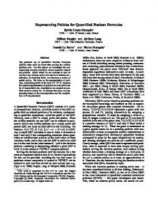
In all the experiments presented so far, we train and test AQME considering the whole set of features, and the results are rewarding. Now we are interested to know (i) whether a subset of the features considered still enables AQME to reach acceptable performances and (ii) whether such features have some relationship with algorithmic differences among its engines. Our main task is thus to isolate a subset of features that are relevant, i.e., such that AQME restricted to these features can reach, or at least get close to, the same performances obtained using the whole set of features. We would like the features in such a set to be model-independent, i.e., relevant for all the models implemented in AQME. Clearly, since different features may be relevant for different models, model-independent features should hint more clearly to the relationships, if any, between properties of QBFs and differences among the engines of AQME. The question then becomes how to find the relevant features, since exhaustive search over 2k subsets of k features is impractical. We consider feature forward selection (FS), a greedy search in the space of possible subsets of features (see, e.g., [19]). FS starts with an empty subset of features. Each feature that is not already in the current subset is tentatively added to it, and the resulting set of features is evaluated using, e.g., cross validation. The effect of adding each feature in turn is quantified, the best one is chosen, and the procedure continues. If no feature produces an improvement, the search ends. Since FS guarantees to find a locally optimal set of features, we compensate for this by considering the sets computed by FS augmented by all the features that are highly correlated with the elements of such sets. We assess correlation using Kendall τ , a coefficient that tests how much the trend of a feature is related to the trend of another. We consider two features to be significantly correlated whenever |τ | ≥ 0.9. Figure 1 (left) contains the results of the above analysis arranged in a matrix, where each cell corresponds to a set obtained by intersecting the subsets of relevant features for any two models implemented in AQME. In each cell, the features marked with a “*” are the ones originally spotted by FS, and mean values are considered for features corresponding to a distribution of values. According to our experiments there are no common relevant features between AQME -MLR and AQME -1NN, and thus no model-independent ones. However, non-empty intersections can be found across R IP PER , C4.5, and 1NN, as well as across R IPPER , C4.5, and MLR. We denote such intersections with F1 and F2 : ∀ wr∀+ wr∀− wr∀− r∀+ r∀− r∀− F1 = { wr wr , wr , wr , wr− , r , r , r− } F2 = {l, l− , p, r∃ , r∃− , vc }
(3)
R IPPER
1NN
R IPPER
C4.5
wr∀− ∗ wr− wr∀+ ∗ r∀+ wr r r∀− r∀− r r− wr∀ wr∀− wr wr
C4.5 wr∀− ∗ wr− r∀+ wr∀ ∗ wr r wr∀+ wr∀− wr wr r∀− r∀ r r r∀− r− ∗ l∗ r∃ p∗ wr∀ ∗ wr wr∀+ ∗ wr l− , r∃+ r+ r∀+ r− vc r r∀− r∀ r r r∀− wr∀− r− wr wr∀− wr−
MLR
–
Solver Q U BE5.0 AQME -R IPPER S K IZZO Q U BE3.0 AQME -MLR SSOLVE
∗ ∗ l ∗ l− p∗ r∃ r∃− vc
2 CLS Q Y Q UAFFLE AQME -1NN AQME -C4.5 QUANTOR QUAFFLE
# 61 58 57 57 53 53 53 51 46 45 45 42
FS Time 1076 335 1379 291 1274 1251 108 84 614 75 42 253
# 61 54 57 57 53 53 53 51 51 55 45 42
M Time 1076 712 1379 291 1219 1251 108 84 625 1083 42 253
FS+M # Time 61 1076 53 1426 57 1379 57 291 53 1013 53 1251 53 108 51 84 51 1176 58 1096 45 42 42 253
∗ ∗ l ∗ l− r∃ p r∃− vc
Fig. 1. Relevant features common to various models implemented in AQME (left) and its engines on the QBFEVAL’07 dataset considering only subsets of features (right).
AQME
vs.
The features in F1 are all variations of the ratio between the average (weighted) number of universal variable occurrences vs. the average (weighted) number of variable occurrences ( rr∀ ). Small (resp. large) values of this ratio indicate that the universal variables tend to occur less (resp. more) than the average. If we consider the runtime distribution of search vs. hybrid solvers on the QBFEVAL’06 dataset, we have that search solvers tend to perform better on small values of rr∀ , while the contrary is true for hybrid solvers. This is probably related to the fact that (a) the QBFEVAL’06 dataset is biased in favor of satisfiable formulas, and (b), for such formulas search solvers tend to spend a lot of time in checking all the combinations of universal variables. Solvers that are not based on search, on the other hand, do perform better on these kind of formulas, as long as they do not apply expansion of universal variables. In the case of weighted occurrences, since outer variables in the prefix have higher weight, either the number of levels is small, or the bulk of existential variables occurrences concerns variables appearing in the outer level of the prefix. Since the median number of quantifier sets in the QBFEVAL’06 dataset is 3 (min. 2, max. 133)6 the first explanation is the one that applies to our results. The features in F2 are related to the distribution of the number of literals per clause (l, and l− ), the distribution of the values of the products between negative and positive occurrences of existential variables (p, and the related r∃ and r∃− ), and the clauses-tovariables ratio ( vc ). If we consider the runtime distribution of search vs. hybrid solvers, we have that search solvers tend to perform better for small values of the above parameters. For l (and l− ), we conjecture that this is related to the fact that in search solvers the number of steps, i.e., variable assignments, required to falsify a clause is proportional to the number of its literals, and thus longer clauses can hurt performances of 6
The corresponding distribution is right-skewed, i.e., it has a long tail on the right, but most formulas have a fairly small number of quantifier sets.
search solvers. In the case of p, search solvers should be relatively insensitive to this parameter, while for solvers based, e.g., on variable elimination by Q-resolution, this parameter gives a rough estimate of the effort required to eliminate a variable. While it is somewhat peculiar that large values of p favor hybrid solvers in the QBFEVAL’06 dataset, considering also the results about vc and other features, we conjecture that this is due to the fact that hybrid solvers are able to solve some of the largest formulas in the dataset, and that this effect may be prevalent over others. In order to check the significance of the features in the subsets F1 and F2 with respect to the whole set of features, we use the QBFEVAL’06 and QBFEVAL’07 datasets to train and test AQME, respectively. We consider F1 ∪ F2 features, as well as others that may discriminate between search and hybrid solvers, and precisely: – The number of quantifier sets s, a rough indicator of complexity. – The mean value of vs∃ and vs∀ , which are related to (i) the number of different Skolem functions, and the size of the parameters of a Skolem function, respectively, as well as (ii) the number of variables to be resolved away with Q-resolution or expanded, respectively (see [15, 14]). – ll∃ and ll∀ which are related to the mean number of variables that could be transformed to a Skolem function, and the mean number of variables that could be expanded with respect to the total variables in a clause; l+ – l− l and l which are related to the size of the antecedent and of the consequent, respectively, looking at each clause as an implication. The results of the above experiment are shown in the table on Figure 1 (right). The organization of the table is the same used for the experiments of Section 5.1. The three groups of columns correspond to considering the features in F1 ∪ F2 alone (FS), the features outlined above (M), or both subsets of features (FS+M). Looking at the table, we can see that in the case of the “FS” selection, only AQME -R IPPER is able to keep up with the best performers in the dataset, namely Q U BE5.0, S K IZZO and Q U BE3.0, while AQME -MLR ranks only fourth best, and AQME -1NN and AQME -C4.5 performances are quite weak. Still, at least for AQME -R IPPER, most of the performances in Table 4, can be explained in terms of F1 ∪ F2 only. In the “M” selection, even if AQME ranks fourth at most, the performances of its four inductive models are more consistent than in the “FS” selection: C4.5, R IPPER, MLR and 1NN solve 55, 54, 53 and 51 problems, respectively. From this, we can see that features that are supposedly linked to the engine internals are more likely to behave in a model-independent fashion. Looking at the “FS+M” selection, we can see that the performances of AQME with the combination of automatic and manual feature selection are very close to the performances that can be obtained using the whole set of features. Even if the performances are still weaker than in Table 4, we are now considering only 20 features out of 141, so it is fair to say that these are the features that matter most in the performances of AQME. In particular, with respect to the results of Table 4, AQME -C4.5 and AQME -1NN have a negative gap of three instances (58 vs. 61 and 51 vs. 54, respectively), while AQME -MLR and AQME R IPPER have a negative gap of 12 and 7 instances, respectively. It is also interesting to notice that while R IPPER, C4.5 and MLR are quite sensitive to changes in the feature space, 1NN performances are not, possibly because of a floor effect.
6
Conclusions
In this paper we have shown that a set of inexpensive syntactic features can hint the choice of the best engine to run on a given QBF. We have provided experimental evidence that our multi-engine solver AQME is a robust alternative to current state-of-theart QBF solvers. We have also shown that AQME is stable with respect to perturbations that may affect the QBFEVAL’06 dataset on which it is engineered. Finally, we have provided some experimental evidence about the significant features leveraged by AQME and their connection with algorithmic differences among its engines. The validation of AQME is still in progress, and further work will include broadening the set of formulas whereon we validate the performances of AQME, the study of dynamic adaptive mechanisms, and a deeper study of the features guiding the choice of the best engine to run on each formula.
References 1. L. J. Stockmeyer and A. R. Meyer. Word problems requiring exponential time. In 5th Annual ACM Symposium on the Theory of Computation, 1973. 2. C. H. Papadimitriou. Computational Complexity. Addison-Wesley, 1994. 3. I.P. Gent, P. Nightingale, and A. Rowley. Encoding Quantified CSPs as Quantified Boolean Formulae. In Proceedings of the 16th European Conference on Artificial Intelligence (ECAI 2004), 2004. 4. T. Jussila and A. Biere. Compressing BMC encodings with QBF. In Proc. 4th Intl. Workshop on Bounded Model Checking (BMC’06), 2006. 5. C. Ansotegui, C.P. Gomes, and B. Selman. Achille’s heel of QBF. In Proc. of AAAI, 2005. 6. U. Egly, T. Eiter, H. Tompits, and S. Woltran. Solving Advanced Reasoning Tasks Using Quantified Boolean Formulas. In Seventeenth National Conference on Artificial Intelligence (AAAI 2000), pages 417–422. The MIT Press, 2000. 7. M. Narizzano, L. Pulina, and A. Taccchella. QBF solvers competitive evaluation (QBFEVAL), 2003-2007. http: //www.qbflib.org/qbfeval. 8. B.A. Huberman, R.M. Lukose, and T. Hogg. An economics approach to hard computational problems. Science, 3, 1997. 9. C.P. Gomes and B. Selman. Algorithm portfolios. Artificial Intelligence, 126, 2001. 10. E. Nudelman, K. Leyton-Brown, A. Devkar, Y. Shoham, and H. Hoos. SATzilla: An Algorithm Portfolio for SAT. In In Seventh International Conference on Theory and Applications of Satisfiability Testing, SAT 2004 Competition: Solver Descriptions, pages 13–14, 2004. 11. H. Samulowitz and R. Memisevic. Learning to Solve QBF. In In proc. of 22nd Conference on Artificial Intelligence (AAAI’07), 2007. 12. M. Davis, G. Logemann, and D. Loveland. A machine program for theorem proving. Communications of the ACM, 5(7):394–397, 1962. 13. H. Kleine-B¨uning, M. Karpinski, and A. Fl¨ogel. Resolution for Quantified Boolean Formulas. Information and Computation, 117(1):12–18, 1995. 14. M. Benedetti. sKizzo: a Suite to Evaluate and Certify QBFs. In 20th Int.l. Conference on Automated Deduction, volume 3632 of Lecture Notes in Computer Science. Springer Verlag, 2005. 15. A. Biere. Resolve and Expand. In Seventh Intl. Conference on Theory and Applications of Satisfiability Testing (SAT’04), volume 3542 of LNCS, 2005. 16. E. Giunchiglia, M. Narizzano, and A. Tacchella. Quantified Boolean Formulas satisfiability library (QBFLIB), 2001. www.qbflib.org. 17. M. Narizzano, L. Pulina, and A. Tacchella. The third QBF solvers comparative evaluation. Journal on Satisfiability, Boolean Modeling and Computation, 2:145–164, 2006. Available on-line at http://jsat.ewi.tudelft.nl/. 18. L. Kaufman and P.J. Rousseeeuw. Finding Groups in Data. Wiley, 1990. 19. I.H. Witten and E. Frank. Data Mining (2nd edition). Morgan Kaufmann, 2005. 20. J. R. Quinlan. C4.5: Programs for Machine Learning. Morgan Kaufmann Publishers, 1993. 21. William W. Cohen. Fast effective rule induction. In Twelfth International Conference on Machine Learning., pages 115–123, 1995. 22. S. Le Cessie and J.C. van Houwelingen. Ridge estimators in logistic regression. Applied Statistics., 41:191–201, 1992. 23. D. Aha and D. Kibler. Instance-based learning algorithms. Machine Learning, pages 37–66, 1991. 24. Ron Kohavi. A study of cross-validation and bootstrap for accuracy estimation and model selection. In In Proc. of Int.l Joint Conference on Artificial Intelligence (IJCAI), 2005.