Sep 6, 2009 - AbstractâFor most diseases and examinations, clinical data such as ... mathematical models such as the Support Vector Machine. (SVM) [15] ... In this paper, the linear .... 3) Final kernel for clinical data: Because each individual ..... similar power in breast cancer prognosis as microarray gene expression.
31st Annual International Conference of the IEEE EMBS Minneapolis, Minnesota, USA, September 2-6, 2009
Development of a kernel function for clinical data Anneleen Daemen and Bart De Moor
Abstract— For most diseases and examinations, clinical data such as age, gender and medical history guides clinical management, despite the rise of high-throughput technologies. To fully exploit such clinical information, appropriate modeling of relevant parameters is required. As the widely used linear kernel function has several disadvantages when applied to clinical data, we propose a new kernel function specifically developed for this data. This “clinical kernel function” more accurately represents similarities between patients. Evidently, three data sets were studied and significantly better performances were obtained with a Least Squares Support Vector Machine when based on the clinical kernel function compared to the linear kernel function.
I. INTRODUCTION When patients undergo an examination, patient-specific information such as age, menopausal status and medical history is registered. Laboratory analyses are performed on for example progesterone, estrogen and CA125. Finally, both histopathological parameters such as tumor size and lymph node status, and ultrasound data such as endometrium thickness may be required. Whilst high-throughput technology has considerably advanced cancer research, for many other diseases and examinations clinical data fully guides clinical management. Furthermore, Eden and colleagues have shown the value of clinical markers over the use of profiles obtained from high-throughput technologies [4]. Advanced mathematical models such as the Support Vector Machine (SVM) [15] can therefore aid clinical decision support by using the available clinical information. In many previous studies, the linear kernel function was used for this purpose [1][8][13]. As will be shown in this manuscript, this kernel function has several disadvantages when applied to clinical data. Our aim is now to present an alternative kernel function specifically developed for clinical data. We will compare both these kernel functions on three clinical data sets, all within the field of anticipation. II. M ETHODS A. Kernel methods and weighted Least Squares Support Vector Machine Kernel Methods, a powerful class of algorithms for pattern analysis, have become a standard tool in data analysis, computational statistics, and machine learning applications due to their reliability, accuracy, and computational efficiency [10]. They have the capability to handle a very wide range of data types (e.g. sequences, vectors, networks) by working in Both authors are with ESAT, Department of Electrical Engineering, Katholieke Universiteit Leuven, Kasteelpark Arenberg 10, 3001 Leuven, Belgium {anneleen.daemen,
bart.demoor}@esat.kuleuven.be
978-1-4244-3296-7/09/$25.00 ©2009 IEEE
a high dimensional feature space. This is obtained with the function Φ(x) which maps the data x from the original input space to the feature space. This embedding is performed by the ’kernel function’ k(xk , xl ), which efficiently computes the inner product hΦ(xk ), Φ(xl )i between all pairs of data items xk and xl in the feature space. This results in the kernel matrix with the size determined by the number of data items. Any symmetric, positive semidefinite function is a valid kernel function (e.g. linear, polynomial, and diffusion kernels). They all correspond to a different transformation of the data, meaning that they extract a specific type of information from the data set. In this paper, the linear kernel function k(xk , xl ) = xTk xl is compared with a newly introduced kernel function for clinical data (see II.B). Both functions were normalized to guarantee a similar order of magnitude for the kernel matrices. A kernel algorithm for supervised classification is the Least Squares Support Vector Machine (LS-SVM), a simplified version of the SVM [15] and developed by Suykens et al. [11][12]. While in many two-class problems data sets are skewed in favour of one class such that the contribution of false negative and false positive errors is not balanced, we used a weighted version of the LS-SVM (wLS-SVM) to account for the unbalancedness in the data sets [7]. The constrained optimization problem has the following form:
min
w,b,e
³
N ´ 1X 1 T ζk e2k , s.t. yk [wT Φ(xk ) + b] = 1 − ek , w w+γ 2 2 k=1 (1)
with ζk =
½
N 2NP N 2NN
if yk = +1 if yk = −1,
NP and NN representing the number of positive and negative samples, respectively, N the total number of samples, ek the error variables tolerating misclassifications in case of overlapping distributions, and γ the regularization parameter which allows tackling the problem of overfitting. We applied a 10-fold cross-validation (CV) approach in which the regularization parameter γ is optimized on a logarithmic scale over an interval from 10−4 to 106 . The optimal γ value was chosen corresponding to the model with the highest 10-fold AUC (area under the ROC curve). If multiple models with equal AUC, the model with the lowest balanced error rate and an as high as possible sum of sensitivity and specificity was chosen. The model with the optimal γ was further validated on an independent test set. For each considered data set, the AUC of the model using the clinical kernel was compared with the AUC of the
5913
models based on the linear kernel function using the method of Hanley and McNeil [6]. B. Kernel function for clinical data A distinction should be made between continuous, ordinal, and nominal variables. Whilst an ordinal variable has two or more categories with an intrinsic ordering, a nominal variable lacks this ordering. A linear kernel function provides a measure of similarity between two patients by calculating their inner product for one or several variables. The inner product for continuous variables depends on the variable range (e.g. age from 20 to 50 years vs. progesterone from 0 to 5 nmol/l). For ordinal variables, the comparison of two patients with value 1 and 2 also depends on the range of this variable. These patients will be less similar when the variable has only three categories then when it has six categories. Furthermore, when a possible category for an ordinal variable equals zero, the inner product for a patient with value zero will always be zero, independent of its dissimilarity with another patient. Finally, for a nominal variable the inner product between two patients should only be larger than zero when both patients have the same category. Therefore, the typically used inner product needs to be redefined. Moreover, because continuous and ordinal variables are not comparable in range, the kernel function needs to be applied to each variable individually. To ascertain the same influence of each variable, the individual matrices need to be normalized before calculating the global, heterogeneous kernel matrix. In the next subsections, an alternative clinical kernel function is proposed for each variable type. The following notations are used: k(xi , xj ) denotes the kernel function for variable x between patients i and j; Kx (i, j) ∀i, j represents the corresponding individual kernel matrix for variable x; K(i, j) ∀i, j represents the global, heterogeneous kernel matrix. 1) Continuous and ordinal clinical variables: The same kernel function is proposed for these variable types: (max − min) − |xi − xj | , (2) max − min with max and min the maximal and minimal value for variable x defined on the training data set. Example 1: We would like to calculate the similarity (i.e., kernel matrix) between three patients h, i, and j for the continuous variable age. Patient h is 23 years old, patient i 26, and patient j 54. Suppose that, based on the training data, the minimal age seems to be 20 and the maximal age 100. The elements in the kernel matrix can then be calculated as follows: kx (i, j) =
Kage (h, i) = (80 − |23 − 26|)/80 = 77/80 Kage (h, j) = (80 − |23 − 54|)/80 = 49/80 Kage (i, j) = (80 − |26 − 54|)/80 = 52/80 The resulting kernel matrix for variable age equals " # Kage =
1 0.9625 0.6125
0.9625 1 0.6500
0.6125 0.6500 1
with values decreasing with increasing dissimilarity between patients. Example 2: The extent of most types of cancer are described with a TNM classification system. The T stands for the size of the primary tumor with possible values 1, 2, 3, and 4. The N describes the degree of spread of the tumor to regional lymph nodes. Simplified, N can be equal to 0 (no spread of tumor cells to regional lymph nodes), 1 (spread to the closest or a small number of lymph nodes), or 2 (spread to more distant or a larger number of lymph nodes). Finally, the absence or presence of metastasis is represented with the binary variable M (see Example 3). Suppose patient h is characterized by T1N0, patient i by T3N2, and patient j by T4N1. The resulting kernel matrices equal # # " " KT =
1 0.33 0
0.33 1 0.66
0 0.66 1
, KN =
1 0 0.5
0 1 0.5
0.5 0.5 1
.
This example illustrates that the proposed kernel function takes the range of variables into account (0.66 vs. 0.5 for a difference in one unit). Furthermore, the kernel value equals zero when two patients are most dissimilar (T1 vs. T4, and N0 vs. N2). The linear kernel function on the other hand would have led to positive values. 2) Nominal clinical variables: For nominal variables, the kernel function between patients i and j is defined as ½ 1 if xi = xj kx (i, j) = . (3) 0 if xi 6= xj This kernel function is independent of the variable values, such that binary, dummy variables are no longer needed. Example 3: Continuing on example 2, we can now apply the kernel function for nominal variables on the variable M. Suppose patient h has no distant metastasis, whilst patients i and j both metastasized to distant organs beyond the regional lymph nodes. In that case, the kernel matrix becomes # " KM =
1 0 0
0 1 1
0 1 1
3) Final kernel for clinical data: Because each individual kernel matrix has been normalized to the interval [0,1], the global, heterogeneous kernel matrix can be defined as the sum of the individual kernel matrices, divided by the total number of clinical variables. This matrix then describes the similarity for a class of patients based on a set of variables of different type. Example 4: The heterogeneous kernel matrix for the similarity between patients h, i, and j based on age, tumor size (T), lymph node spread (N), and metastasis (M) is given by # " K=
5914
1 (Kage +KT +KN +KM ) = 4
1 0.324 0.2781
0.324 1 0.7042
0.2781 0.7042 1
C. Clinical data sets We considered three clinical data sets for which a distinction was made between continuous variables (labeled as C), ordinal variables (O), and nominal variables (N). Endometrial disease: Data set I contains clinical information on 402 patients with an endometrial disease who underwent an echographic examination and color Doppler [14]. The patients are divided into two groups according to their histology: malignant (hyperplasia, polyp, myoma, and carcinoma) versus benign (proliferative endometrium, secretory endometrium, atrophia). After excluding patients with incomplete data, the data was, stratified to outcome, randomly divided into a training and test set. The training set contains two-third of the masses, i.e., 226 of which 109 malignant and 117 benign; the test set contains the remaining one-third (113 masses, 54 malignant and 59 benign). An overview of the 24 clinical variables is given in Table I. Miscarriages: A prospective observational study of 1828 women undergoing transvaginal sonography before 12 weeks gestation resulted in data for 2356 pregnancies of which 1458 normal at week 12 and 898 miscarriages during the first trimester [2]. When randomly dividing the data set stratified to outcome, the training set contains 1571 pregnancies of which 972 normal and 599 miscarriages, and the test set 785 pregnancies with 486 normal and 299 miscarriages. The 18 clinical variables are shown in Table II. Pregnancies of Unknown Location: Data set III contains data on 1003 pregnancies of unknown location (PUL) [5]. Within the PUL group, there are four clinical outcomes: a failing PUL, an intrauterine pregnancy (IUP), an ectopic pregnancy (EP) or a persisting PUL. Because persisting PULs are rare (18 cases in the data set), they were excluded, as well as pregnancies with missing data. The final data set consists of 856 PULs among which 460 failing PULs, 330 IUPs, and 66 EPs. As the most important diagnostic problem is the correct classification of the EPs [3], we divided the data into a training set containing 571 pregnancies (527 non-EP, 44 EP) and a test set with 285 pregnancies (263 non-EP, 22 EP). The 15 clinical variables are shown in Table III. The ranges of the variables shown in Tables I to III were determined based on the training data. III. R ESULTS A. Comparison of the linear and clinical kernel function In a first phase, we verified whether the clinical kernel function better represents the true similarity between the samples. For this purpose, a publicly available data set on breast cancer was used in which the appearance of distant subclinical metastases was predicted based on the primary tumour [16]. This data set of 148 patients contains 13 clinical parameters: 2 continuous parameters, i.e., age (20-60 years) and tumour diameter (0-70 mm); 4 ordinal parameters, one ranging from 0 to 15, the others from 1 to 3; and 7 nominal, binary parameters. Fig. 1 shows the histograms of the kernel matrices based on the linear and clinical kernel function, with the continuous variables being standardized for the linear kernel.
TABLE I C LINICAL VARIABLES DATA SET I variable 1. age (years) 2. weight (kg) 3. number of miscarriages/abortions 4. parity 5. gravidity 6. menopausal status 7. hormonal therapy 8. intrauterine device 9. type of AUBρ 10. amount of AUBρ 11. duration of AUBρ (months) 12. endometrial cells 13. endometrium thickness on USψ (mm) 14. intracavity fluid (mm) 15. 3-layer pattern 16. intracavity lesion 17. subendometrial cyst 18. endometrial cyst 19. number of calcifications 20. number of myoma 21. ovary aspect 22. number of follicles 23. pedicle sign 24. endometrium thickness on CD² (mm) ρ AUB, abnormal uterine bleeding ψ US, ultrasound ² CD, color Doppler
type C C O O O N N N N N C N C C N N N N O O N N N C
range 22 - 85 45 - 160 0-5 0-6 0-7 1,2,3 0-4 0,1,2 1,2,3 1,2,3 0.5 - 96 1,2,3 0 - 39.4 0 - 8.7 1,2 1,2,3 1,2 1,2 0-8 0-4 1,2 0,1 1,2,3 0 - 47.8
TABLE II C LINICAL VARIABLES DATA SET II variable 1. age (years) 2. PBAC bleeding score 3. follow-up consent 4. ethnicity 5. regular dates 6. gravida 7. number of deliveries after 24 weeks 8. number of terminated pregnancies 9. number of early miscarriages 10. number of PULsρ 11. number of late miscarriages 12. number of ectopic pregnancies 13. previous chromosomal abnormalities 14. bleedingψ 15. painψ 16. previous ectopic pregnancyψ 17. previous miscarriageψ 18. anxietyψ ρ PUL, pregnancy of unknown location ψ indication for scan
type C O N N N O O O O O O O N N N N N N
range 15 - 48 0-4 0,1,2 0-6 0,1,2 1 - 12 0 - 10 0-4 0 - 10 0-1 0-5 0-1 0,1 0,1 0,1 0,1 0,1 0,1
The histogram for the linear kernel function has a slightly larger mean equal to 0.7410 (median 0.7766) compared to a mean of 0.7122 (median 0.7168) for the clinical kernel function. Four comparisons on the patients shown in Table IV were made to verify whether differences in the kernel values correspond to true differences in patient data. Comparison a) Minimal clinical kernel value: Patients 55 and 84 are most dissimilar according to the clinical kernel function with a kernel value of 0.1523 contrary to 0.1415 for the linear kernel function (see Table IV for the clinical parameters). These two patients differ greatly in tumour size (C2 ), are most different for three of the four
5915
TABLE III C LINICAL VARIABLES DATA SET III
TABLE IV S PECIFIC PATIENT DATA FROM [16]
1200
1200
1000
1000
800
800
nb of occurrences
nb of occurrences
variable type range 1. hCGρ at 0h (U/l) C 1.79 - 9.15ψ 2. progesterone at 0h (nmol/l) C 0 - 5.25ψ 3. hCGρ at 48h (U/l) C 0 - 9.52ψ 4. progesterone at 48h (nmol/l) C 0 - 5.25ψ 5. hCGρ ratio (48h/0h) C 0.085 - 4.77 6. endometrium thickness (mm) C 1.5 - 34.9 7. character of midline echo N 0,1 8. free fluid in pouch of Douglas N 0,1 9. gestational age (days) C 10 - 100 10. lower abdominal pain N 0,1 11. vaginal bleeding N 0,1,2 12. previous miscarriage N 0,1 13. previous ectopic pregnancy N 0,1 14. anxiety N 0,1 15. age (years) C 14 - 49 ρ hCG, human chorionic gonadotropin ψ on a logarithmic scale after correction for a positively skewed distribution
600
400
200
0
600
400
200
0
0.2
0.4
0.6 K(i,j)
(a) Linear kernel
0.8
1
0 0.1
0.2
0.3
0.4
0.5
0.6
0.7
0.8
0.9
1
K(i,j)
(b) Clinical kernel
Fig. 1. Histograms of the kernel matrices: (a) based on the linear kernel function after standardization of the continuous variables, (b) based on the clinical kernel function.
ordinal variables (O2 to O4 ), and have different values for all nominal variables. Comparison b) Minimal linear kernel value: The lowest value for the linear kernel function on the other hand occurs between patients 36 and 55 and is equal to 0.0089, in contrast to the clinical kernel value of 0.3904. When comparing the data of these two patients, age and tumour size seem to be more different than was the case in comparison a. These patients, however, are equal for two ordinal and two nominal variables. The clinical kernel function ranks these patients as more similar due to the equal weights given to each variable. In the linear kernel, however, the influence of the continuous variables age and tumour size dominates the influence of the non-continuous variables. Comparison c) Influence of ordinal and nominal variables: For validating the influence of the non-continuous variables on the kernel matrix, we chose three patients with the same age and tumour size (see Table IV). Patients 1 and 18 are different according to two nominal variables, whilst patients 1 and 45 slightly differ in two ordinal variables (0 vs. 1 for O1 on a range from 0 to 15, and 1 vs. 2 for O2 on a range from 1 to 3). Taking into account the range of the variables, patients 1 and 45 are more similar than patients 1 and 18. This difference in similarity is much clearer with the clinical kernel function (0.9564 and 0.8462, respectively) compared to the linear kernel function (0.9465 and 0.9313,
Patient
55
a 84
36
b 55
1
c 18
45
6
58
d 3
79
C1 C2 O1 O2 O3 O4 N1 N2 N3 N4 N5 N6 N7
50 8 0 1 3 1 0 1 0 0 0 0 0
41 45 4 3 1 3 1 0 1 1 1 1 1
37 50 0 1 1 3 1 0 0 0 1 1 1
50 8 0 1 3 1 0 1 0 0 0 0 0
41 20 0 1 1 3 0 1 0 0 1 1 0
41 20 0 1 1 3 1 0 0 0 1 1 0
41 20 1 2 1 3 0 1 0 0 1 1 0
40 14 0 1 1 3 0 1 0 0 1 1 0
39 15 0 1 1 3 0 1 0 0 1 1 0
48 15 0 1 1 3 0 1 0 0 1 1 0
49 16 0 1 1 3 0 1 0 0 1 1 0
respectively). Comparison d) Influence of continuous variables: Finally, we compared four patients with the same ordinal and nominal variables but some minor differences in age and tumour size. Patients 6 and 58 differ 1 year in age with a difference of 1 mm in tumour size. The same differences hold for patients 3 and 79, but they are both older with a slightly larger tumour. The similarities k(6, 58) and k(3, 79) are both equal to 0.9970 for the clinical kernel function. These similarities, however, are slightly different according to the linear kernel function (0.9983 and 0.9984). B. Results on real data Subsequently, we compared the linear and clinical kernel function on three data sets when used in a supervised classification algorithm. A 10-fold cross-validation (CV) approach was applied to train a wLS-SVM model, which was subsequently validated on a test set. These results are shown in Table V, the ROC curves of the models when applied on the test sets in Fig. 2. Significant differences between models based on the clinical kernel function and the corresponding models based on the linear kernel function (with and without standardization of the continuous variables) are indicated in bold at a significance level of 0.05. The wLS-SVM based on the clinical kernel function outperformed the wLSSVMs based on the linear kernel function, although not significant in all cases. For data set II, there was a significant improvement for the training set, whilst significantly better results were obtained on the test set from data set III. IV. CONCLUSIONS When modeling clinical data, good results can be obtained with the linear kernel function when the variables with the largest range correlate better with the predicted outcome, as larger weights are assigned to such variables. However, when the reverse is true, this linear kernel function is not optimal. Because the correlation is often unknown beforehand, because nominal variables with numerous categories can distort the calculation of patient similarity, and moreover, to eliminate dependency on variable ranges, each variable must have the same influence on the calculation of patient
5916
TABLE V R ESULTS ON REAL DATA Data set I
II
III
10-fold AUC
linear linear std clinical linear linear std clinical linear linear std clinical
0.7431 0.7425 0.7608 0.7392 0.7464 0.7702 0.8034 0.8130 0.8602
0.4768 0.4470
0.7216 0.7423 0.8107 0.7718 0.7729 0.7840 0.8177 0.8225 0.9231
6.36e-4 0.0059 0.0438 0.0747
p-valueµ 0.0455 0.0523 0.3588 0.3624 5.51e-5 6.61e-5
R EFERENCES
comparison with the AUC of the clinical kernel function[6]
100
100
90
90
80
80
70
70
60
60
50 40
50 40
30
30
20
20
10 0
test AUC
p-valueµ
Sensitivity
Sensitivity
µ
Kernel function
- Flanders (FWO-Vlaanderen). BDM is a full professor at the Katholieke Universiteit Leuven, Belgium. This work is partially supported by: 1. Research Council KUL: GOA AMBioRICS, CoE EF/05/007 SymBioSys, PROMETA, several PhD/postdoc & fellow grants. 2. Flemish Government: a. FWO: PhD/postdoc grants, projects G.0241.04, G.0499.04, G.0318.05, G.0302.07, research communities (ICCoS, ANMMM, MLDM); b. IWT: PhD Grants, GBOU-McKnow-E, GBOU-ANA, TAD-BioScope-IT, Silicos; SBO-BioFrame, SBO-MoKa, TBM-Endometriosis. 3. Belgian Federal Science Policy Office: IUAP P6/25 (BioMaGNet). 4. EURTD: ERNSI; FP6-NoE Biopattern; FP6-IP e-Tumours, FP6-MCEST Bioptrain, FP6-STREP Strokemap.
10 0
20
40 60 1 − Specificity
80
0
100
0
20
(a) Data set I
40 60 1 − Specificity
80
100
(b) Data set II
100 90 80
Sensitivity
70 60 50 40 30 20 10 0
0
20
40 60 1 − Specificity
80
100
(c) Data set III Fig. 2. ROC curves of the wLS-SVM models applied on the test sets (linear kernel, blue solid line; linear std kernel, black dotted line; clinical kernel, red dashed line).
similarities, which is not the case. We therefore propose the clinical kernel function which takes into account the type and range of each variable. This requires the specification of each type of variable, as well as the minimal and maximal possible value for continuous and ordinal variables based on the training data or on a priori knowledge. Notably, the test data may contain more extreme values for certain variables. This is, however, irrelevant as the kernel matrix remains positive semi-definite with only negative values besides the diagonal, expressing more dissimilarity with the training cases. From our results, we can conclude that the clinical kernel function more accurately represents similarities between patients. Moreover, the wLSSVM based on the clinical kernel function significantly outperformed the linear kernel function when tested on three data sets.
[1] Adjouadi M, Zong N, Ayala M. (2005) Multidimensional pattern recognition and classification of white blood cells using support vector machines. Part Part Syst Charact, 22, 107-118. [2] Bottomley C, Daemen A, et al. (2009) Functional linear discriminant analysis: a new longitudinal approach to the assessment of embryonic growth. Hum Reprod, 24, 278-283. [3] Condous G, Okaro E, et al. (2004) The use of a new logistic regression model for predicting the outcome of pregnancies of unknown location. Hum Reprod, 19, 1900-1910. [4] Ed´en P, Ritz C, et al. (2004). ”Good old” clinical markers have similar power in breast cancer prognosis as microarray gene expression profilers. Eur J Can, 40, 1837-1841. [5] Gevaert O, De Smet F, et al. (2006) Predicting the outcome of pregnancies of unknown location: Bayesian networks with expert prior information compared to logistic regression. Hum Reprod, 21, 18241831. [6] Hanley JA, McNeil BJ. (1983) A method of comparing the areas under receiver operating characteristics curves derived from the same cases. Radiology, 148, 839-843. [7] Cawley GC. (2006) Leave-one-out cross-validation based model selection criteria for weighted LS-SVMs. Proc. of IJCNN, 1661-1668. [8] Majumder SK, Ghosh N, Gupta PK. (2005) Relevance vector machine for optical diagnosis of cancer. Lasers Surg Med, 36, 323-333. [9] Sch¨olkopf B, Tsuda K, Vert JP. (2004) Kernel methods in computational biology, MIT Press, United States. [10] Shawe-Taylor J, Cristianini N. (2004) Kernel methods for pattern analysis, Cambridge University Press, Cambridge. [11] Suykens JAK, Vandewalle J. (1999) Least Squares Support Vector Machine classifiers, Neural Processing Letters, 9, 293-300. [12] Suykens JAK, Van Gestel T, et al. (2002) Least Squares Support Vector Machines, World Scientific, Singapore. [13] Van Calster B, Timmerman D, et al. (2007) Preoperative diagnosis of ovarian tumors using Bayesian kernel-based methods. Ultrasound Obstet Gynecol, 29, 496-504. [14] Van den Bosch T, Daemen A, et al. (2007) Mathematical decision trees versus clinician based algorithms in the diagnosis of endometrial disease. Ultrasound Obstet Gynecol, 30, 412. [15] Vapnik V. (1998) Statistical Learning Theory, Wiley, New York. [16] van de Vijver M, He Y, et al. (2002) A gene-expression signature as a predictor of survival in breast cancer. N Engl J Med, 347, 1999-2009.
V. ACKNOWLEDGMENTS AD is research assistant of the Fund for Scientific Research
5917