kernel estimation of cumulative distribution function of a random ...

STATISTICS IN TRANSITION new series, September 2016

541

STATISTICS IN TRANSITION new series, September 2016 Vol. 17, No. 3, pp. 541–556

KERNEL ESTIMATION OF CUMULATIVE DISTRIBUTION FUNCTION OF A RANDOM VARIABLE WITH BOUNDED SUPPORT Aleksandra Baszczyńska1 ABSTRACT In the paper methods of reducing the so-called boundary effects, which appear in the estimation of certain functional characteristics of a random variable with bounded support, are discussed. The methods of the cumulative distribution function estimation, in particular the kernel method, as well as the phenomenon of increased bias estimation in boundary region are presented. Using simulation methods, the properties of the modified kernel estimator of the distribution function are investigated and an attempt to compare the classical and the modified estimators is made. Key words: boundary effects, cumulative distribution function, kernel method, bounded support.

1. Introduction Nonparametric methods are becoming increasingly popular in statistical analysis of economic problems. In most cases, this is caused by the lack of information, especially historical data, about the economic variable being analysed. Smoothing methods concerning functions, such as density or cumulative distribution, play a special role in a nonparametric analysis of economic phenomena. Knowledge of density function or cumulative distribution function, or their estimates, allows one to characterize the random variable more completely. Estimation of functional characteristics of random variables can be carried out using kernel methods. The properties of the classical kernel methods are satisfactory, but when the support of the variable is bounded, kernel estimates may suffer from boundary effects. Therefore, the so-called boundary correction is needed in kernel estimation.

1

Department of Statistical Methods, University of Łódź. E-mail: [email protected].

542

A. Baszczyńska: Kernel estimation of cumulative …

Kernel estimator of cumulative distribution function has to be modified when the support of the variable is defined as a,  ,  , b or a, b . Such a situation is frequently observed in an economic analysis, for example, when data are considered only on the positive real line (e.g.: arable land, energy use, CO2 emission, external debts stocks, current account balance, total reserves, etc.). Near zero, the classical kernel distribution function estimator is poor because of its considerable bias. The bias comes from the behaviour of kernel estimator, which has no knowledge of the boundary and assigns probability on the negative real line. A range of boundary correction methods for kernel distribution function estimator is present in the literature. They are addressed mainly to boundary kernels (Tenreiro, 2013; Tenreiro, 2015) and reflection method (Koláček, Karunamuni, 2009; Koláček, Karunamuni, 2012). In Section 2 we introduce the kernel method, which for the first time was implemented in density estimation in the late 1950s. The properties of the kernel density estimator, as well as the modifications, are presented taking into account the boundary effects reduction of classical kernel density estimator. In Section 3 some selected methods of distribution function estimation are presented, including the kernel method. Some methods of choosing the smoothing parameter of kernel method and properties of estimator are shown, and methods of boundary correction are used in the case of cumulative distribution function estimation. In Section 4 the results of a simulation study are given and an attempt to compare the considered estimators is made. In addition, the comparison of the values of smoothing parameters is presented. The simulations and the plots were carried out using MATLAB software. The aim of the paper is to give a detailed presentation of methods of the modified kernel distribution function estimation and to compare the considered methods. The simulation shows that when boundary correction is used in kernel estimation of distribution function, the estimator has better properties.

2. Kernel method The kernel method originated from the idea of Rosenblatt and Parzen dedicated to density estimation. The Rosenblatt-Parzen kernel density estimator is as follows (cf.: Härdle, 1994; Wand, Jones, 1995; Silverman 1996; Domański et al., 2014):

1 fˆn ( x )  nhn

n

 x  Xi   ,  hn 

 K  i 1

(1)

where: X 1 , X 2 ,..., X n is the random sample from the population with unknown

density function f x  ; n is the sample size; hn is the smoothing parameter, which controls the smoothness of the estimator ( lim h  0 , lim nh   ). n 

n 


543

Throughout this paper the notation h  hn will be used. K u  is the weighting function called the kernel function. When K u  is symmetric and unimodal function and the following conditions are fulfilled:   K u du  1,      uK u du  0,     u 2 K u du    0, 2   

 

(2)



the kernel function is called the second order kernel function (or classical kernel function). 1  1  The most frequently used Gaussian kernel function K u   exp   u 2  2  2  is a function belonging to this group, although its support is unbounded. It stands in contrast to other kernel functions fulfilling conditions (2), like functions presented in Table 1, for which support is bounded. The indicator function I  u  1 is defined as follows: I  u  1  1 for u  1 , I  u  1  0 for u  1 . Table 1. Kernel functions Kernel function

K u 

Uniform

1 I  u  1 2

Triangle

1  u I  u  1

Epanechnikov





3 1  u 2 I  u  1 4









Quartic

2 15 1  u 2 I  u  1 16

Triweight

3 35 1  u 2 I  u  1 32

Cosine

 4

  cos u  I  u  1 2 


544

Higher order kernel functions (the order of the kernel is the order of the first nonzero moment) can be used, especially in reducing the mean squared error of the estimator. But the higher order kernels properties may sometimes be unacceptable because they may result in taking negative values for the density function estimators. When the support of random variable is, for example, left-bounded (support of random variable is 0,  ), the properties of the estimator (1) may differ in boundary region 0, h and in inner region h,  (cf.: Jones, 1993; Jones, Foster, 1996; Li, Racine, 2007). The estimator (1) is not consistent in boundary region. As a result, the support of the kernel density estimator may differ from the support of the random variable and the estimator may be non-zero for negative values of random variable. Moreover, this situation may appear when the kernel function has unbounded as well as bounded support. Removing boundary effects can be done in various ways. The best known and most often used method is the reflection method, which is characterized by both simplicity and best properties. Assuming that the support of random variable is 0,  , the reflection kernel density estimator, based on reflecting data about zero, has the following form (cf. Kulczycki, 2005):

1 fˆnR ( x )  nh

  x  Xi   x  Xi   K h   h i 1 n

 K 

  . 

(3)

The estimator (3) is a consistent estimator of unknown density function f . Moreover, it integrates to unity and for x close to zero the bias is of order O (h ) . The analysis of the properties of this estimator is presented in Baszczyńska (2015), among others.

3. Distribution function estimation Let X1, X 2 ,..., X n denote independent random variables with a density function f and a cumulative distribution function F . One can estimate the cumulative distribution function (CDF) by: 1 Fˆn  x   n

n

 I

, x 

X i  ,

(4)

i 1

where I A is the indicator function of the set A: I A ( x )  1 for x  A , I A ( x)  0 for x  A . The empirical distribution function defined by (4) is not smooth, at each point

X 1  x1 , X 2  x2 ,..., X n  xn it jumps by

1 . n

545


The smoothed version of the empirical distribution estimator is the Nadaraya kernel estimator of CDF:

1 Fˆ ( x )  n

n

x Xi h

 

K  y dy 

i 1  

1 n

n

 x  Xi h

W  i 1

 , 

(5)

where h is a smoothing parameter such as lim h  0 , lim nh   and n 

n 

x



W ( x )  K (t )dt . Assuming that function K ( x )  0 is a unimodal, symmetric 1

kernel function of the second order with support  1,1 (examples of these kernels are presented in Table 1), the properties of function W (x ) are the following: W ( x )  0 for x   ,1,

W ( x )  1 for 1



x  1,  ,

1



W 2 ( x )dx  W ( x )dx  1 ,

1

(6)

1 1

 W ( x) K x dx  2 , 1

1

1  1 xW ( x ) K  x dx  1  W 2 ( x )dx  . 2  1  1 1





Function W (x ) is a cumulative distribution function because K (x ) is a probability density function. For example, when the kernel function is Epanechnikov kernel, the function W (x ) has the form:

0 for x  1,  1 3 1  W  x    x 3  x  for 4 2  4 1 for x  1.

x  1,


546

Assuming additionally that F ( x ) is twice continuously differentiable, the mean integrated squared error (MISE) of kernel distribution estimator (5) is as follows: 

   Fˆ x   F x  dx 

MISE Fˆ  x   E

2



(7) 



1 h h  F  x 1  F  x dx  c1  c2 h 4  o  h 4 , n  n n 



where: 1



c1  1  W 2 (t )dt ,

(8)

1

c2 

 22 4



   F t  dt , 2

2

(9)



F  s  denotes the sth derivative of the cumulative distribution function.

Kernel distribution estimator (5) is a consistent estimator of the distribution function. The expectation value, bias and variance are, respectively:





 

1 E Fˆ x   F  x   F 2  x h 2 2  o h 2 , 2





 

1 B Fˆ x   F 2  x h 2 2  o h 2 , 2  1  h 1 1 D 2 Fˆ  x   F  x 1  F  x   hf  x 1  W 2 (t )dt   o  . n n  1   n 







The method of choosing the value of the smoothing parameter in kernel estimation of the cumulative distribution function is of crucial interest, as it is in kernel estimation of the density function. Some procedures used frequently in CDF estimation are presented in Table 2.

547


Table 2. Methods of choosing the smoothing parameter in kernel estimation of the cumulative distribution function Method

Smoothing parameter

hˆCV  arg min CV h  , hH n

Cross-validation, CV

1 CV (h)  n

n 

  I  i 1  

 , x 

 X i   Fˆi x, h  dx , 2

Fˆi x, h  is a kernel estimator based on the sample with X i deleted Maximal smoothing principle, MSP

Plug-in, PI

hMS

 7c    12   15 2 

1

3

 c1   hPI   2   ˆ1 2 

n 1

1

3

n

7ˆ 2

3

1

3

, ˆ k g  

n  Xi  X j  1  , L2 k   2 g n g i , j 1  



g is an initial smoothing parameter, L2k  is the 2kth derivative of the initial kernel function L hIT , j 1  Iteration, IM

4hIT , j c1n

n

 Xi  X j   , j  0,1,... , hIT , j 



i , j 1 i j

u   K  K W W  2 K W W  W W u  ,

f  g denotes convolution

When the random variable has bounded support (without loss of generality one can take 0,  ), as in the case of the kernel density estimation, the properties of the kernel distribution function get poorer, in comparison with the situation when the support is unbounded. For x in boundary region x  0, h , let c  x / h , 0  c  1 , the expectation value and the variance of estimator (5) are the following:


548

c

 

ˆ B E F  x   F  x   hf 0  W ( t ) dt 



1 c c  c 2   h 2 f 1 0   c W (t )dt  tW (t )dt   o h 2 ,  2  1 1



 



c 2  1 1 ˆ F  x 1  F  x   hf 0  W (t )dt  c   oh . B D F x   n n  1  2







It is to note that in boundary region the estimator is not consistent, but variance is of the same order. The reflection kernel distribution estimator has the form (cf. Horovà et al., 2012):

1 FˆR ( x )  n

  x  Xi   x  Xi  W  h   h i 1 n

 W 

  . 

(10)

The generalized reflection kernel distribution estimator, improving the bias of the estimator and holding onto low variance, is the following (cf. Karunamuni, Alberts, 2005; Karunamuni, Zhang, 2008):

1 FˆGR ( x )  n

  x  g1  X i    x  g 2  X i    W   , h h    i 1 n

 W 

(11)

where g1 and g 2 are cubic polynomials with such coefficients that the bias of the

  2

estimator is of order O h . In boundary region the expectation value and variance of the estimator (11) are, respectively:





E FˆGR  x  

 F x  

c c c c    c2   h 2  f 1 0  2c W (t )dt  tW (t )dt   f 0g12  0 c  t W (t )dt  f 0g 22  0 c  t W (t )dt    1 c 1 1  2 









 

 o h2 , c c c  1 1 D 2 FˆGR  x   F  x 1  F  x   hf 0 W 2 (t )dt  2 W (t )W (t  2c )dt  W 2 (t )dt   oh  . n n 1 1  1 












549

4. Results of the simulation study The objective of the simulation study was to compare properties of chosen estimators of the distribution function. The estimators were considered in a special situation when the support of the random variable is bounded. The comparison was made through the graphical representation of the results of the estimation. This form of presenting the estimator is of crucial importance, especially from the user’s point of view. The graph provides a fast, comprehensive and readable form of presenting the functional characteristic of the random variable, even for inexperienced users. In the simulation study the following populations with Weibull distribution W 0, ,  with different scale and shape parameters were examined:

W 10,1,0.1 , W 20,1,0.5 ,

W 30,1,1 , W 40,1,2 , W 50,1,3.4 , W 60,1,5 , W 70,4,1 , W 80,4,2 . The use of a wide range of distribution parameters ensures that varied populations are considered in the study. The difference between populations can be seen, for example, in location, dispersion, asymmetry and kurtosis. The samples X1, X 2 ,..., X n of size n  10,20,...,100 were drawn from each population and the following estimators of the distribution function were calculated: empirical distribution function (4), kernel distribution function (5) and reflection kernel distribution function (11). For kernel estimators, Gaussian, Epanechnikov and quartic kernels were used, with Silverman’s practical rule (RR), maximal smoothing principle (MSP), plug-in method (PI) and iteration method (IM) used for choosing the smoothing parameter. Some results for medium size sample n  50 drawn from selected populations, where Epanechnikov kernel and Silverman’s rule were used in kernel estimators, are presented in Figures 1-8.


550

Empirical distribution function 1 0.9 0.8 0.7 0.6 0.5 0.4 0.3 0.2 0.1 0 -5

0

5

10

15

20

25

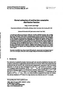
Figure 1. Empirical distribution function, sample size n  50 from W 20,1,0.5 population

1

1

0.9

0.9

0.8

0.8

0.7

0.7

0.6

0.6

0.5

0.5 0.4

0.4

0.3

0.3

0.2

0.2

0.1

0.1 0 -5

0 -5

0

5

Kernel estimator

10

15

20

0

5

10

15

20

25

25

Reflection kernel estimator

Figure 2. Kernel distri bution function estimators, sample size n  50 from W 20,1,0.5 population

551


Empirical distribution function 1 0.9 0.8 0.7 0.6 0.5 0.4 0.3 0.2 0.1 0 -0.5

0

0.5

1

1.5

2

2.5

3

3.5

4

Figure 3. Empirical distribution function, sample size n  50 from W 30,1,1 population

1

1

0.9

0.9

0.8

0.8

0.7

0.7

0.6

0.6

0.5

0.5

0.4

0.4

0.3

0.3

0.2

0.2

0.1

0.1

0 -0.5

0

0.5

Kernel estimator

1

1.5

2

2.5

3

3.5

0 4 -0.5

0

0.5

1

1.5

2

2.5

3

3.5


Figure 4. Kernel distribution function estimators, sample size n  50 from W 30,1,1 population

4


552

Empirical distribution function 1 0.9 0.8 0.7 0.6 0.5 0.4 0.3 0.2 0.1 0

0

0.2

0.4

0.6

0.8

1

1.2

1.4

1.6

1.8

Figure 5. Empirical distribution function, sample size n  50 from W 50,1,3.4 population

1

1

0.9

0.9

0.8

0.8

0.7

0.7

0.6

0.6

0.5

0.5

0.4

0.4

0.3

0.3

0.2

0.2

0.1

0.1

0

0

0.2

0.4

Kernel estimator

0.6

0.8

1

1.2

1.4

1.6

0 1.8 0

0.2

0.4

0.6

0.8

1

1.2

1.4


Figure 6. Kernel distribution function estimators, sample size n  50 from W 50,1,3.4 population When the group of samples from populations with the same scale parameter but with shape parameter differences (populations W 10,1,0.1 – W 60,1,5 ) is considered, it can be noticed that the lower the value of shape parameter, the bigger the incompatibility between the support of the random variable and the

1.6

1.8

553


support of the kernel distribution function estimator. For high values of shape parameters (for example, in populations W 40,1,2 – W 60,1,5 ) the influence of boundary effects is almost imperceptible. When samples are drawn from populations with high values of shape parameters, kernel functions, used in constructing the distribution function estimator in observations near zero, do not extend beyond the support of the random variable. Empirical distribution function 1 0.9 0.8 0.7 0.6 0.5 0.4 0.3 0.2 0.1 0 -1

0

1

2

3

4

5

6

7

8

9

Figure 7. Empirical distribution function, sample size n  50 from W 80,4,2 population

1

1

0.9

0.9

0.8

0.8

0.7

0.7

0.6

0.6

0.5

0.5

0.4

0.4

0.3

0.3

0.2

0.2

0.1 0 -1

0.1 0

1

2

Kernel estimator

3

4

5

6

7

8

9

0 -1

0

1

2

3

4

5

6

7

8


Figure 8. Kernel distribution function estimators, sample size n  50 from W 80,4,2 population

9


554

It is worth stressing that when Gaussian kernel function was used in kernel estimator, the boundary effects were bigger, in comparison with other kernel functions. This results directly from the properties of Gaussian kernel which is the only one among the studied kernel functions that has unbounded support. The kernel distribution function estimators behave in a very similar way, even for very small samples (n=10, n=20). Hence, the sample size is not the essential factor in the occurrence of boundary effects. Taking into account the values of shape parameters and sample sizes, the same results were observed when for the same populations with bounded random variable, the kernel density function estimators were constructed (cf. Baszczyńska, 2015). However, it must be indicated that boundary effects influence the shape of estimators more strongly in the case of density estimator, in some cases even giving the wrong impression of multimodality. To extend the study, the dependence between kernel function and smoothing parameter was observed. The results are presented in Table 3. Table 3. Values of smoothing parameters in kernel distribution function estimation for samples from Weibull distribution populations Method of smoothing parameter choice Population

Kernel function RR

W 10,1,0.1

W 20,1,0.5 W 30,1,1

W 40,1,2  W 50,1,3.4  W 60,1,5 W 70,4,1 W 80,4,2 

MSP

PI

IM

Epanechnikov

0.8635

0.9224

0.2655

quartic

1.0203

1.0899

0.3137

Epanechnikov

1.0958

1.1706

0.3878

0.1872

quartic

1.2948

1.3832

0.4582

0.2638

Epanechnikov

0.5852

0.6251

0.4817

0.4974

quartic

0.6914

0.7386

0.5692

0.5699

Epanechnikov

0.3792

0.4051

0.4105

0.4199

quartic

0.4481

0.4787

0.4851

0.4885

Epanechnikov

0.2771

0.2961

0.3523

0.3267

quartic

0.3275

0.3498

0.4162

0.3858

Epanechnikov

0.2265

0.2419

0.3178

0.2645

quartic

0.2676

0.2859

0.3756

0.1986

Epanechnikov

3.0632

3.2722

0.7626

1.8332

quartic

3.6195

3.8666

0.9011

2.1697

Epanechnikov

1.9802

2.1154

0.7755

1.6573

quartic

2.3399

2.4996

0.9163

2.0212


555

In the procedure of kernel estimation of cumulative distribution function, two kernel functions: Gaussian and Epanechnikov functions, influence the kernel estimator in a very similar way. The application of these kernel functions is connected with almost the same values of smoothing parameters. It can indicate that Gaussian and Epanechnikov kernels have similar smoothing properties, although they are characterized by different support. When quartic kernel is used, the smoothing parameter is smaller in comparison with other kernel functions. For samples from populations with small shape parameter, the kernel distribution estimator with smaller smoothing parameters was used. The bigger the shape parameter, the bigger the smoothing parameter in kernel estimation. In general, using Silverman’s reference rule ensures smaller values of smoothing parameter. When the shape parameter of population distribution is small, the iterative method is rather poor, the smoothing parameter is unacceptably big, which is denoted by a grey spot in Table 3.

5. Conclusion The kernel method is an intuitive, simple and useful procedure, especially in density and distribution function estimation. When the support of the random variable is bounded, this procedure needs modification. The modified kernel distribution function estimator ensures that the estimator is consistent, even in boundary region, and the support of the estimator is the same as the support of the random variable being analysed. In kernel method two parameters should be predetermined: kernel function and smoothing parameter. Quartic kernel function indicates higher values of smoothing parameter. Silverman’s reference rule, though based on the assumption that the population distribution is normal, gives smaller values of the smoothing parameter.

REFERENCES BASZCZYŃSKA, A., (2015). Bias Reduction in Kernel Estimator of Density Function in Boundary Region, Quantitative Methods in Economics, XVI, 1. DOMAŃSKI, C., PEKASIEWICZ, D., BASZCZYŃSKA, A., WITASZCZYK, A., (2014). Testy statystyczne w procesie podejmowania decyzji [Statistical Tests in the Decision Making Process], Wydawnictwo Uniwersytetu Łódzkiego, Łódź. HÄRDLE, W., (1994). Applied Nonparametric Regression, Cambridge University Press, Cambridge. LI, Q., RACINE, J. S., (2007). Nonparametric Econometrics. Theory and Practice, Princeton University Press, Princeton and Oxford.

556


JONES, M. C., (1993). Simple Boundary Correction for Kernel Density Estimation, Statistics and Computing, 3, pp. 135–146. JONES, M. C., FOSTER, P. J., (1996). A Simple Nonnegative Boundary Correction Method for Kernel Density Estimation, Statistica Sinica, 6, pp. 1005–1013. KARUNAMUNI, R. J., ALBERTS, T., (2005). On Boundary Correction in Kernel Density Estimation, Statistical Methodology, 2, pp. 191–212. KARUNAMUNI, R. J., ZHANG, S., (2008). Some Improvements on a Boundary Corrected Kernel Density Estimator, Statistics and Probability Letters, 78, pp. 497–507. KOLÁČEK, J., KARUNAMUNI, R. J., (2009). On Boundary Correction in Kernel Estimation of ROC Curves, Australian Journal of Statistics, 38, pp. 17–32. KOLÁČEK, J., KARUNAMUNI, R. J., (2012). A Generalized Reflection Method for Kernel Distribution and Hazard Function Estimation, Journal of Applied Probability and Statistics, 6, pp. 73–85. KULCZYCKI, P., (2005). Estymatory jądrowe w analizie systemowej [Kernel Estimators in Systems Analysis], Wydawnictwa Naukowo-Techniczne, Warszawa. HOROVÀ, I., KOLÁČEK, J., ZELINKA, J., (2012). Kernel Smoothing in MATLAB. Theory and Practice of Kernel Smoothing, World Scientific, New Jersey. SILVERMAN, B.W., (1996). Density Estimation for Statistics and Data Analysis, Chapman and Hall, London. TENREIRO, C., (2013). Boundary Kernels for Distribution Function Estimation, REVSTAT Statistical Journal, 11, 2, pp. 169–190. TENREIRO, C., (2015). A Note on Boundary Kernels for Distribution Function Estimation, http://arxiv.org/abs/1501.04206 [14.11.2015]. WAND, M. P., JONES, M.C., (1995). Kernel Smoothing, Chapman and Hall, London.