D.B. Das and V. Nassehi Chemical Engineering Department, Loughborough University, Loughborough LE11 3TU, Leicestershire, UK. (E-mail:
[email protected]) Abstract The interfaces between free (e.g., groundwater) and porous (e.g., soil) flow zones in the subsurface represent important transition zones across which many important transfer/exchange processes occur. The understanding of these interactive phenomena and the way these regions behave in combination is, therefore, critical for management of subsurface water quality. Indispensable to this is numerical modelling and simulation as they can handle complex flow domains and minimise the analysis cost and time. In the present work, the hydrodynamic conditions for a combined free and porous flow domain in the subsurface are analysed. An investigation into the fluid dynamical behaviour for different aspect ratios of the domains is of most interest. Keywords Aspect ratio; combined flow in subsurface; finite volume method; interface
Introduction
Fluid flow through combined free and porous pathways in the underground systems is a common transport phenomenon. In many instances, such coupled flow behaviour is observed due to artificial objects/structures in the subsurface. The permeable reactor barrier (PRB) in the subsurface for remediation of contaminated groundwater is a case in point. Other underground engineering processes, such as dig-and-treat and pump-and-treat methods for groundwater treatment, and extraction of oil from underground reservoirs also involve coupled free and porous flow regions. However, in a great majority of the cases, the associated fluid transport phenomena are observed due to the natural hydro-environmental conditions, such as seepage through preferential flow domains, rise and fall of groundwater and flow circulation. In general, the sub-domains in the coupled flow systems are distinguished by an interfacial surface, which represents an important transition zone for fluid mobility. Flow models for such combined areas require descriptions of not only the fluid dynamical characteristics in the individual domains but also the mass and momentum transfer behaviour across the interfaces. For simplicity of the fluid dynamical analyses, these phenomena are often classified as microscopic and macroscopic transport processes (Das and Nassehi, 2001). The impact of the combined flow on the overall transport behaviour depends on many distinguishing features such as the dimensions of the pathways, its behaviour in combination with the surroundings, and the characteristics of the porous material, e.g., the porosity and the permeability. The number of permeable interfaces between the free and the porous flow domains, and the aspect ratios of the sub-domains also influence the fluid dynamics. To model fluid flow in these domains, two approaches are usually adopted: firstly, the formulations based on an assumption of continuum domains and secondly, the formulations based on discrete pathways. In the former case, the porous section is treated as a pseudofluid layer and the whole domain is considered to be a single domain. As such, one suitably formulated equation of motion in conjunction with other equations for continuity of mass and pollutant specie balance is solved. The mathematical model recognises the free and the porous flow domains based on a spatially varying permeability. Such a single-domain
Water Science and Technology Vol 45 No 9 pp 301–307 © 2002 IWA Publishing and the authors
Development of a new mathematical model for subsurface water quality management
301
D.B. Das and V. Nassehi 302
approach is usually preferred in systems where the flow transition from free to porous flow sections is not distinct and the structural properties of the permeable domain progressively change. Application of this approach is most commonly found in the metal solidification problems involving mushy zones. However, if the permeability of the porous media is relatively high and constant, so that the interface between adjacent free and porous media forces a transition from free to porous flow, or vice versa, the whole domain must be viewed as a combination of adjacent flow fields rather than a continuous single domain. In such transport phenomena, the second approach should be utilised where the appropriate equations of motions describing the flow in different sub-domains are used. Mathematical models based on the multi-domain approach for most combined flows are well established for artificial flow systems (Nassehi and Petera, 1994; Gartling et al., 1996; Gobin et al., 1998; Nassehi, 1998; Chen et al., 1999). However, extensions of these formulations to the composite flow in the underground have been uncertain. The main difficulty in this task is the realistic representation of flow behaviour at the interfacial surface, which stems from two main sources. The first one is the inherent irregularity in the size and shape of the domains. Secondly, the randomness can be related to a generalised lack of knowledge about the processes involved and the impossibility of an exhaustive analytical description. In the case of combined free and porous flow in the subsurface, not only the interface is expected to have random shape and size but also there is a complete lack of physical evidence for the mass and momentum transport behaviour across the interface. Therefore, to preserve the compatibility of the underground fluid dynamical characteristics at the interfaces, numerical schemes are usually used as they can deal with such problems. It is well known that the finite element schemes can readily cope with curved and complex problem domains (Nassehi and Petera, 1994; Gartling et al., 1996; Nassehi, 1998). However, realistic modelling of the underground flow processes requires three-dimensional computations, which become excessively expensive if the finite element methods are used. Other numerical techniques that can, apparently, resolve such difficulties due to their inherent mathematical strength are, for example, the finite volume (Patankar, 1980; Versteeg and Malalasekera, 1995) and the spectral (Canuto et al., 1988; Guo, 1998) methods. These methods should, therefore, be adopted for representing the underground fluid flow (Das and Nassehi, 2001; Das et al., 2001a; Das et al., 2001b). A two-domain mathematical model that can be used for combining three dimensional (3-D) zones of permeable soil domains and free flow channels is described in the present paper. The permeable domain is assumed to be a continuum medium and the average macroscopic flow properties, such as velocity and pressure, are evaluated on the representative elementary volumes (REVs). The present study deals with such a combined flow system for which there is a complete lack of experimental/field data, particularly for interfacial flow properties, to compare them directly with the predicted values. The finite volume method (FVM) is, therefore, adopted in the present work for discretising the governing flow equations to algebraic forms and solving them as it can conserve fluid materials at each grid cell unlike other numerical methods. Though, in general, the computational costs of using the spectral method is less than that of the FVM for the same spatial scale, due to the above advantage the present mathematical formulation is based on the standard finite volume technique instead of the spectral method. In doing so, the physical region of combined flow is truncated to a computational domain where the boundary conditions necessary for solving the problem are imposed. Results presented in this paper represent the hydrodynamic conditions for a physical water flow process. In particular, the influence of the aspect ratios of the combined domain on the flow based on different thicknesses of the porous layer is analysed. The developed model, in effect, provides a prerequisite hydrodynamical model for predicting the contaminants mobility in
combined domains of free and porous flow in the subsurface. It is envisaged that the present treatment of subsurface water flow would make predictions for water quality in the underground zones more accurate and realistic. Formulation of the mathematical model
∇Pf = −ρ
∇Pp = −ρ
Dv f + µ∇2 v f Dt ∂v p ∂t
−
D.B. Das and V. Nassehi
As mentioned before, the present work is based on a two-domain flow model for simultaneously simulating the hydrodynamics of combined water flow in the subsurface. The Navier-Stokes equation (equation 1) is adopted as the governing equation for the momentum transfer in the free flowing fluid while the flow in the porous domain is represented by the Darcy equation (Eq. 2). Validity of these equations in the respective cases is well known. Constant properties of the fluid are also assumed. The non-dimensional governing equations for motion, as adopted in this work, are as follows, (1)
µ vp K
(2)
where, the subscript “f” and “p” refer to the free and the porous flow domains. P and v are the pressure and velocity field, respectively, while ρ and µ are, respectively, the constant density and viscosity of the fluid. K is the second order tensor representation of the isotropic permeability in the porous medium. The equations of continuity for conservation of mass in both free and permeable domains are represented as, ∇.ve = 0
e ≡ f, p
(3–4)
The three components of the velocity field in the longitudinal (x–), lateral (y–) and the vertical (z–) directions are designated as u, v and w. As the matching interfacial condition for linking the equations of motion, the modified form of Beavers and Joseph (1967) formulation is used (Das et al., 2001a). For a Darcian flow region, Beavers and Joseph proposed an empirical slip-flow boundary condition at the interface describing the proportionality between the shear rate at the interface and the slip velocity through a dimensionless slip coefficient that depends only on the structural properties of the interface. The validity of the formulation has been verified through both theoretical modelling studies (Saffman, 1971) and experiments (Beavers et al., 1970). Applicability of the formulation to different combined flow regimes has been tested by, among others, Salinger et al. (1993, 1994), Gobin et al. (1998) and Das et al. (2001a). As adopted in this work, the interfacial boundary conditions are (Das and Nassehi, 2000; Das et al., 2001a), Longitudinal velocity component, u
: uf = up
(5)
Lateral velocity component, v
γ yz ∂v ∂u vf − v p + = : K yy ∂x ∂y f
Transverse velocity component, w
γ yz ∂w ∂u : wf − w p + = ∂x ∂z f K zz
(
(
)
(6)
)
(7) 303
γ yz ∂w ∂u : wf − w p + = ∂x ∂z f K zz
(
Pressure, P
)
(8)
D.B. Das and V. Nassehi
where γyz is a slip co-efficient at the interfacial surface characterised by only its structural properties. Kyy and Kzz are the components of the permeability tensor in the lateral (y–) and the transverse (z–) directions. The boundary conditions imposed for the solution of the hydrodynamic equations in the present work consist of inlet and initial boundary conditions for velocity and pressure. At the exit, “no boundary condition” or “open boundary condition” is imposed to handle the stress free section of the domains. As mentioned before, the governing equations are discretised and reduced to algebraic forms using the finite volume method in this work. The temporal discretisation of the equations for predicting the transient flow behaviour is based on the explicit method. The detailed descriptions of the type of grid used in this study and the derivation of the working equations have been described elsewhere (Das and Nassehi, 2001; Das et al., 2001a). They are, therefore, not repeated here for the brevity of the paper. Numerical results and discussions
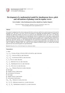
As mentioned before, the combined flow system in the subsurface is influenced by a large number of factors and as such, general analyses of the problem cannot be done. In the present framework, the fluid dynamics of combined flow for different aspect ratios of the domains is considered. A detailed analysis of the associated flow in the subsurface for a global aspect ratio (x:y:z :: 1:1:1) has been presented by Das et al. (2001) where the hydrodynamics of the characteristic flow at different sections of the domains, i.e. free flow, porous flow and the interface was investigated. The investigation revealed that water in the free flow section has a unidirectional path, in general. On the other hand, water moves in from the open portion of the porous domain and reverses its direction at the free/porous flow interface. However, the front of velocity reversal and the centre of circulation move away from the interface with time. After a certain interval the flow in the porous domain becomes unidirectional and moves towards the exit of the domain. Figure 1 (a and b) presents typical profiles of free and porous flow for an aspect ratio of x:y:z :: 1:1:1 at time level 25. The longitudinal (x–) co-ordinate of the interface is “45” and it lies at the y–z plane. The flow reversal occurs because of a complex pressure differential across the interface in specific and the combined flow domain in general (Das et al., 2001). However, with change in the aspect ratios of the domain, different patterns of velocity reversal may be observed. In Figure 2, typical velocity fields in the porous section for an
45 41 37 33 29 25 21 17 13 9
45 41 37 33 29 25 21 17 13 9 41
37
41 37 33 33
29
29
25
25
21
21
17
17 13
13 9
9
45 41 37 33 29 25 21 17 13 9
45 41 37 33 29 25 21 17 13 9 41
37
77 73 69 33
65
29
61
25
57
21
53
17 49
13 9
(a) Free flow section – xf:y:z :: 1:1:1, t=25 304
45
(b) Porous flow section – xp:y:z :: 1:1:1, t=25
Figure 1 Individual velocity profiles in sub-domains of combined free and porous flow regions in subsurface
45 41 37 33 29 25 21 17 13 9
45 41 37 33 29 25 21 17 13 9 41
37
77 73 69
41
37
65
29
77 73 69 33
61
25
65
29
61
25
57
21
53
17
57
21
53
17 9
45
9
49
13
49
13
(a) Porous flow section - x:y:z :: 0.5:1:1, t=25
45
(b) Porous flow section - x:y:z :: 0.5:1:1, t=45
Figure 2 Velocity profiles in the porous flow region in the subsurface
D.B. Das and V. Nassehi
33
45 41 37 33 29 25 21 17 13 9
45 41 37 33 29 25 21 17 13 9
aspect ratio of xp:y:z :: 0.5:1:1 for the porous domain is shown at two time levels t = 25 and t = 45. In effect, it presents a case where the thickness of the porous domain has been reduced to half. Therefore, velocity profiles correspond to a large extent to the profiles presented in Figure 1 for the permeable section. The aspect ratio of the free flow section is xf:y:z :: 1:1:1 in this instance and the velocity profile therein is the same as the previous case. The interfacial velocity across the interface is the same for both aspect ratios above and is presented in magnified form in Figure 3 (a and b) for two time levels t = 25 and t = 45. The velocity fields in this work are predicted at the cell nodes. Therefore, the velocity fields are not presented at the interface (x co-ordinate “45”). As evident, the front of flow reversal is observed near the interface at time level 25 which moves away at time level 45. With reduced thickness of the domain in the lateral direction (y–), the front of velocity reversal becomes much less mobile. The amount of water flowing towards the interface increases with time, which may make the interfacial velocity unstable. Such trends for an aspect ratio of xf,p:y:z :: 1:0.5:1 at time level 25 and 45 have been presented in Figure 4 (a and b). A comparison between the velocity profiles in Figures 3 and 4 indicates clearly that the front has moved away from the interface in the former case but not in the latter case. Also, the velocity distribution in Figure 4(b) is of particular interest as the fluid at the interface begins to be unstable. Hence, the possibility arises for water in the porous section to move to the free flow section due to the greater pressure at the porous side of the interface. Similar observations are also made if the transverse length of the domain is minimised. Figure 5 presents two typical profiles to illustrate the phenomena for an aspect ratio of
45 41 37 33 29 25 21 17 13 9
45 41 37 33 29 25 21 17 13 9 41
45 41 37 33 29 25 21 17 13 9
45 41 37 33 29 25 21 17 13 9 41
37
33
29
45 25
37
45.5 33
45
29 25 21
21
44.5
17
17
13
13
9
9
44
44
(a) (i) xf:y:z :: 1:1:1, xp:y:z :: 1:1:1, t=25 (ii) xf:y:z :: 1:1:1, xp:y:z :: 0.5:1:1, t=25
(b) (i) xf:y:z :: 1:1:1; x p:y:z :: 1:1:1, t=45 (ii) xf:y:z :: 1:1:1; xp:y:z :: 0.5:1:1, t=45
Figure 3 Velocity profiles across the free/porous interface in the subsurface
305
45 41 37 33 29 25 21 17 13 9
45 41 37 33 29 25 21 17 13 9 41
45 41 37 33 29 25 21 17 13 9
45 41 37 33 29 25 21 17 13 9 41
D.B. Das and V. Nassehi
37
33
37
33
45
29
45
29 25
25
21
21
17
17
13
13 9
9
44
(a) xf,p:y:z :: 1:0.5:1, t=25
44
(b) xf,p:y:z :: 1:0.5:1, t=45
Figure 4 Velocity profiles across the free/porous interface in the subsurface
45 41 37 33 29 25 21 17 13 9
45 41 37 33 29 25 21 17 13 9 41
45 41 37 33 29 25 21 17 13 9
45 41 37 33 29 25 21 17 13 9 41
37
33
45
29
37
33
45
29 25
25
21
21
17
17
13
13 9
9
44
(a) xf,p:y:z :: 1:1:0.5, t=25
44
(b) xf,p:y:z :: 1:1:0.5, t=45
Figure 5 Velocity profiles across the free/porous interface in the subsurface
Conclusions
The 3-D velocity profiles for a combined free and porous flow region in the subsurface have been presented. Due to the complex pressure distributions in the free/porous interface, the fluid reverses its directions. The aspect ratios of the domains play a significant role in determining the locations of the centre of flow circulation and the front of flow reversal. In many cases, the fronts of flow reversal move away with time from the interfacial surface. But there is no universal physical significance to such flow phenomena as with different aspect ratios, the pattern may change. It can, therefore, be concluded that the scales of the domain determine the flow reversal and other important factors such as rate of fluid circulation. This, in turn, necessitates that each independent case of combined water flow in the subsurface is investigated based on the specific problem domains for the management of underground water quality. Acknowledgement
Prof. R.J. Wakeman of the Chemical Engineering Department, Loughborough University, UK, is acknowledged for his comments during the preparation of this manuscript. B.G. Technology, UK is acknowledged for providing the necessary funds to carry out this work. References
306
Beavers, G.S. and Joseph, D.D. (1967). Boundary conditions at naturally permeable wall. Journal of Fluid Mechanics, 30, part 1, 197–207. Beavers, G.S., Sparrow, E.M. and Magnuson, R.A. (1970). Experiments on coupled parallel flows in a
D.B. Das and V. Nassehi
channel and bounding porous media. Journal of Basic Engineering, Transaction of the ASME, 92D, 843–848. Canuto, C., Hussaini, M.Y., Quarteroni, A. and Zang, T.A. (1988). Spectral methods in fluid dynamics, Springer-Verlag, New York, 1988. Chen, Q.-S., Prasad, V. and Chatterjee, A. (1999). Modelling of fluid flow and heat transfer in a hydrothermal crystal growth system: use of fluid-superposed porous layer theory. Journal of Heat Transfer, Transaction of the ASME, 121, 1049–1058. Das, D.B. and Nassehi, V. (2000). Computational methods in the modelling and simulation of pollutants’ mobility in contaminated lands – a review of the physical flow processes. In: Recent Advances in Chemical Engineering, S.G. Pandalai (ed.), vol 4, Transworld Research Network, Trivandrum, pp. 117–136. Das, D.B. and Nassehi, V. (2001). LANDFLOW: A 3D finite volume model of combined free and porous flow of water in contaminated land sites. Water Science and Technology 43(7) 55–64. Das, D.B., Nassehi, V. and Wakeman, R.J. (2001a). A finite volume model for the hydrodynamics of combined free and porous flow in sub-surface regions. Advances in Environmental Research (in press). Das, D.B., Kafai, A. and Nassehi, V. (2001b). Application of spectral expansions to modelling of underground water flow. Accepted for presentation in the “3rd International Conference on Future Groundwater at Risk, 25–27 June, 2001, Lisbon, Portugal”. Gartling, D.K., Hickox, C.E. and Givler, R.C. (1996). Simulation of coupled viscous and porous flow problems. Computational Fluid Dynamics, 7, 23–48. Gobin, D., Goyeau, B. and Songbe, J.-P. (1998). Double diffusive natural convection in a composite fluidporous layer. Journal of Heat Transfer, Transaction of the ASME, 120, 234–242. Guo, B.-Y. (1998). Spectral methods and their applications, River Edge, N.J.: World Scientific, Singapore. Nassehi, V. (1998). Modelling of combined Navier-Stokes and Darcy flows in crossflow membrane filtration. Chemical Engineering Science, 53(6), 1253–1265. Nassehi, V. and Petera, J. (1994). A new least-squares finite element model for combined Navier-Stokes and Darcy flows in geometrically complicated domains with solid and porous boundaries. International Journal of Numerical Methods in Engineering, 37, 1609–1620. Patankar, S.V. (1980). Numerical heat transfer and fluid flow. Hemisphere, Washington DC. Saffman, P.G. (1971). On the boundary condition at the surface of a porous material. Studies in Applied Mathematics, 50, 93–101. Salinger, A.G., Aris, R. and Derby, J.J. (1993). Modelling the spontaneous ignition of coal stockpiles. AIChE Journal, 40(6), 991–1004. Salinger, A.G., Aris, R. and Derby, J.J. (1994). Finite element formulations for large-scale coupled flows in adjacent porous and open fluid domains. International Journal for Numerical Methods in Fluids, 18, 1185–1209. Versteeg H. K. and Malalasekera W. (1995). An introduction to computational fluid dynamics: the finite volume method. Addision Wesley Longman Ltd., Essex.
307