The effects of ramp rates on the suppliers' benefits have been demonstrated through numerical examples simulated in the simulator. It is shown that, in a.
DEVELOPMENT OF A POWER POOL SIMULATOR G. B. Shrestha
Song Kai
L.K. Goel
School of Electrical and Electronic Engineering Nanyang Technological University, Singapore Abstract Power pool has emerged as one of the preferred modes for organizing an electricity market. Design and development of a power pool simulator for the study of competitive power market is presented in this paper. More choices and options are provided to the power suppliers and customers to encourage competition. The effects of ramp rates on the suppliers’ benefits have been demonstrated through numerical examples simulated in the simulator. It is shown that, in a competitive power market, power suppliers can optimize their benefits by providing proper bidding data; and that power suppliers have tradeoffs between benefits and risks. The fact that more benefits are accompanied by more risks in competitive power market is illustrated. 1.
INTRODUCTION
Since the reform of the electricity industry in England and Wales started in the late 1980s, it has been seen the trend towards the deregulation and restructuring in electricity industries all over the world, which has resulted in the creation of electricity markets in a number of countries [1]. As a clearinghouse for the market participants (power suppliers and customers), power pool has emerged as one of the most acceptable options for organizing an electricity market. Each deregulated electricity market is structured differently and continues to go through different phases of restructuring. The degree of deregulation and competition is a policy choice in different nations and even in different states of one country [2]. Thus the structures and functions of power pools are also not identical. This paper presents the design of a market-oriented power pool simulator and the study of some issues using the designed simulator. The simulator incorporates features which provide more freedom and options to the participants to create more competition in the power market. We believe that the trend is towards inducing more choice and more competition in the electricity industry. In the power pool simulator, double-side bids are adopted. Both power suppliers and customers are allowed to submit their priceenergy bidding curves. Power suppliers can provide information about willingness to commitment, minimum up time and ramp rate values for every hour within the capacities of their facilities. In the competitive power market, the bidding values specified by the power suppliers are expected to use as strategies so that they can optimize their benefits. This paper is organized as follows. Section 2 presents and explains the features of the power pool simulator. Section 3 outlines the theoretical models used in the simulator. Section 4 describes an example to
demonstrate the operation process of the simulator. Section 5 presents a specific example, which demonstrates the effect of ramp rates on the suppliers’ benefits. Section 6 summarizes our conclusions. 2.
BASIC FEARTURES
The simulator is designed for power pools with the following main features. •
The model adopts a day ahead trading beginning at midnight. The power trading is based on the bids submitted by the market participants. Thus it is a price-based operation.
•
The market price is cleared for each hour of trading period of up to 24 hours.
•
The functions of dispatching, scheduling and market price clearing are integrated with the simulator. Therefore, in the model, the power pool has the responsibility of not only balancing the system supply and demand but also of operating the power system.
•
Double side bids are adopted. One of the most commonly discussed issue about the different power market structures is whether buyers should submits bids, or only the demand forecasts should be used in power pools. We deem that the buyers are an important part of the competitive process and should be encouraged to develop competition. Thus in the model, demand side bidding (DSB) is allowed to increase the degree of participation by the customers.
•
Both power suppliers and customers provide the bid curves for energy in the form of piece-wise linear curves with three stages. A power supplier can also submit bidding for reserve capacity.
•
In the power pool model, the values of the power facilities’ parameters need not be the same as
their physical values. Power suppliers submit the values of the ramp rate limits for every hour and the minimum up time to optimize their benefits. However, this does not mean that suppliers can follow their whims to provide bidding data. For example, if a supplier provides its ramp rates beyond the real capacity of its facilities, it may be possible for the supplier to gain benefit owing to the capacity committed as spinning reserve although it can not, in reality, provide so much capacity. Obviously this situation is forbidden and should be penalized. Therefore, some measures should be taken to check the capacity of the suppliers’ facilities at regular intervals. The bidding data must be within the real capacity of the suppliers’ facilities. •
•
Power suppliers specify their willingness to commit themselves. If a supplier does not want to commit in a certain hour, it is certain that it will not be committed in that hour. However, it can not be ensured that the supplier be committed in a certain hour even though it wants to commit in that hour. In this case, whether a supplier is committed or not depends on the supply and demand in the electricity market. During the process of dispatch, those suppliers who do not want to commit at a certain hour will not be considered at that hour. Thus it is expected that the task for dispatch will be reduced. It is assumed that a supplier’s bidding prices include the incremental cost, no load cost and start up cost. In this case, the cost recovery is left to power suppliers themselves. Power suppliers are expected to get cost recovery and optimize their benefits through their bidding data.
Figure 1 shows the linear piece-wise bidding curves with three stages for the market participants. It should be noted that even in the market environment, not all the customers are willing to submit different bidding data for every hour of every day. In terms of the customers’ sensitivities to the power price, we classify the customers into three categories: • Price-robust: The bid prices for the three stages are the same. • Price-subsensitive: The bid prices of the two stages are the same. • Price-sensitive: The bid prices of the three stages are all different. Some customers would rather make long–term contract with power supplier companies. These customers should belong to the first category, price-
robust customers. When these customers are included in the model, they can be regarded as those submitting high price for all the three stages. From this point of view, the model has a common format. Price ($) Price3 Price2 Price1 P (MW) 0 Min. Output
Elbow1 Elbow2 Max. Output
(a) Bidding curve of suppliers
Price ($) Price1 Price2 Price3 0
P (MW) Elbow1 Elbow2 Max. Load
(b) Bidding curve of customers Figure 1. Bidding curves for the market participants Price ($/MW) Aggregated customer bidding curve
Aggregated supplier bidding curve P (MW) Figure 2. The market clearing process
Figure 2 shows the process of obtaining marketclearing price. The aggregated supplier-bidding curve is obtained by adding all the curves of all the power suppliers. Similarly, by adding all the curves of all the power customers, the aggregated customer-bidding curve is obtained. The intersection point of the two curves is the clearing point. Corresponding to the clearing point, the highest price of the committed suppliers is the cleared price for suppliers, while the lowest price of the committed customers is the cleared price for customers. Generally, the two cleared prices are not the same. There are different ways of determining the final market clearing price. In our study, we simply define the average value of the two cleared prices as the final market clearing price to share the market benefits among the power participants.
Objective function: 3.
THE MODEL
The basic formulation of the power pool simulator is described in this section. The following are the symbols and notations used: i: j: k: t: ST:
Index for the number of suppliers or customers Index for the number of bidding stages Index for the number of nodes Index for the number of time periods(hours) Number of stages of a bid. In our study, ST=3 since bidding curve has three stages N: Number of nodes T: Number of hours SG(t): Set of supplier bids at hour t SL(t): Set of consumer bids at hour t SG(k,t): Set of supplier bids at bus k at hour t SL(k,t): Set of consumer bids at bus k at hour t SR(t): Set of supplier spinning reserve bids at hour t GMW(i, j, t): MW of generation stage j by supplier i at hour t GP(i, j, t): Price of generation stage j by supplier i at hour t LMW(i, j, t): MW of load stage j by consumer i at hour t LP(i, j, t): Price of load stage j by consumer i at hour t RMW(i, t): MW of spinning reserve by supplier i at hour t RP(i, t): Price of spinning reserve by supplier i at hour t Pb(t): Vector of branch flows at hour t B: Matrix of branch sensitivity coefficients with respect to node injection power Pn(t): Vector of node injection power Pn(k, t): The kth element of vector Pn(t) Vector of branch line capacity limits at hour t Pb : u (i, t ) : Zero-one decision variable indicating whether supplier i is up or down at hour t max PG (i, j , t ) : Maximum output of stage j by supplier i at hour t min PG (i, j , t ) : Minimum output of stage j by supplier i at hour t max PG (i ) : Maximum output limits of supplier i PLmax (i, j , t ) : Maximum load demand of stage j by consumer i at hour t max PR (i, t ) : Maximum available spinning reserve by supplier i at hour t RD(i , t ) : Ramp down limit of supplier i at hour t RU (i, t ) : Ramp up limit of supplier i at hour t R (t ) : Spinning reserve requirement at hour t
The objective is to maximize the difference between customers’ benefits from purchases of electricity and the cost of production of electricity and spinning reserve provided. This is consistent with the objective of maximizing social benefits (the sum of the gains deriving from an activity or project to whomsoever they accrue) from the viewpoint of economic theory. The objective function is expressed as follows: max ∑ { ∑ t∈T
∑ LMW (i , j , t ) * LP (i, j , t )
i∈S L ( t ) j∈ST
− ∑
∑ u (i, t ) * GMW (i, j , t ) * GP (i , j , t )
i∈SG ( t ) j∈ST
− ∑ u (i, t ) * RMW (i, t ) * RP(i , t ) i ∈S R ( t )
}
(3.1)
This is to be maximized subject to the following system constraints at every hour: (1) Line flow equations Pb (t ) = BPn (t )
3.2)
Active power flows of lines are expressed as a function of node injection power. (2) Node injection power at bus k Pn (k , t ) =
∑
∑ GMW (i, j , t )
i∈SG ( k ,t ) j∈ST
− ∑
∑ LMW (i, j , t )
(3.3)
i∈S L ( k ,t ) j∈ST
(3) Load balance equation ∑
∑ GMW (i, j , t ) − ∑
i∈S G ( t ) j∈ST
∑ LMW (i , j , t ) = 0
i∈S L (t ) j∈ST
(3.4) (4) Line Capacity limits − Pb ≤ Pb (t ) ≤ Pb
(3.5)
(5) Bid limits PGmin (i, j , t ) ≤ u (i , t ) * GMW (i, j , t ) ≤ PGmax (i, j , t ) 0 ≤ LMW (i, j , t ) ≤ PLmax (i , j , t ) 0 ≤ u (i , t ) * RMW (i , t ) ≤ PRmax (i , t )
(3.6~3.8)
Where, PRmax (i , t ) = min(PGmax (i ) − ∑ GMW (i , j , t ), j∈ST
RU (i, t ))
(3.9)
periods as 8 to demonstrate the operation process of the power pool simulator.
(6) Reserve requirements ∑ u(i, t ) * RMW (i, t ) ≥ R(t )
i∈S R (t )
(3.10) Gen 1 Load 1
R(t) is the larger between the largest generator output of the supplier and the 10% of the total system demand.
1
2
Gen 2
Gen 3
4
3
6
2 Gen 7
1 3
(7) Ramp rate constraints
5
Gen 4 Load 2
RD(i , t ) ≤ u (i, t ) * ∑ GMW (i, j , t ) − u(i, t − 1) j∈ST
* ∑ GMW (i, j , t − 1) ≤ RU (i , t )
11
12 7
10
5
8
11
Load 5
(3.11)
j∈ST
Load 7
13
9
12
It can be seen that the optimization problem is coupled for a number of hours. In addition, all the control variables consisting of the bidding MW amounts of generation and spinning reserve of suppliers and load of customers have upper and lower limits as is evident from (3.6~3.8). These variables are bounded variables. Dynamic Programming (DP) method with restricted search path [3] is adopted to solve the above coupled problem. Interior point (IP) methods is used to solve the optimization problems by starting with a point in the interior of the feasible region and continuing through the interior towards the boundary solution. As a highly efficient method especially for large-scale LP problems, the Primal Affine Scaling approach (a variant of the IP methods) with Phase-Two strategy is adopted to solve the LP problem for every hour. In addition, based on the feature of the bounded variables, a simpler Primal Affine Scaling method for phase II algorithm is presented in [4]. The simple and efficient formulation for phase I algorithm and for the potential push method are derived to improve the computational efficiency, which are presented elsewhere. 4.
MARKET OPERATION : AN EXAMPLE
A 14 bus, 8-supplier and 7-customer system shown in Figure 3 is used to illustrate the operation process of the power pool simulator. The system configuration is obtained from [5] by adding one more supplier. And reasonable values for the network parameters such as the resistance and the inductance per km of the lines are assumed. The bidding data are designed by the authors to create suitable system operation conditions. For illustrative purpose, we take the number of the
8
14
(8) Minimum up and down time limits All the suppliers are subjected to the minimum up and down time limits.
4
6 Load 3
7
Gen 5
10
9
Load 4 Gen 8
Load 6 Gen 6
Figure 3. The example system Tables 5.1 and 5.2 show the formats of the bidding data for the market participants used in the sikulator. Table 5.1 Bidding data of suppliers for one hour Supplier No. 1 2 3 4 5 6 7 8 Commit or not 1 1 1 1 1 1 0 1 Price1($/MW) 8.14 8.08 8.34 11.35 11.38 8.36 13.41 5.39 Price2($/MW) 8.58 8.46 8.81 11.66 11.71 8.88 13.78 5.65 Price3($/MW) Elbow1(MW) Elbow2(MW) RU(MW/hour) RD(MW/hour)
8.93 200 300 1200 1200
8.81 200 300 1200 1200
9.25 200 300 1200 1200
where RU: ramp up rate
11.97 100 150 600 600
12.02 100 150 600 600
9.32 14.09 5.87 200 40 300 300 80 450 1200 600 1800 1200 600 1800
RD: ramp down rate
For every hour, power suppliers should submit their bidding data in the format as shown in Table 5.1. In addition, the minimum up and down time are specified by the suppliers one time. In fact, the minimum output and maximum output can also be provided for every hour by power suppliers. For power customers, they should submit their bidding data for every hour in the format as shown in Table 5.2. Table 5.2 Bidding data of customers for one hour Consumer No. 1 Price1($/MW) 50 Price2($/MW) 50 Price3($/MW) 8.45 Elbow1(MW) 200 Elbow2MW) 230 Maxi. load(MW) 260
2 50 50 50 100 100 100
3 50 50 8.73 200 230 270
4 50 9.01 8.64 120 160 280
5 50 8.57 8.44 130 150 160
6 50 50 8.8 150 180 220
7 15.5 13 8.5 50 80 100
Cleared
Compared to the traditional process of scheduling and dispatching, the power pool model has a larger amount of data to deal with.
2500 power 2000 1390 1500 1000 500 0 1
A sample of simulation results for one hour as shown in Tables 5.3, 5.4 and 5.5.
1700
1750
2
3
2080
4
1860
5
1745
6
1500
1400
7
8 hour
Cleared power
Table 5.3 Results about suppliers for one hour Supplier No. 1 2 3 Power(MW) 200 200 200 Price($/MW) 8.14 8.08 8.34 Reserve(MW) 200 200 200
4 0 0 0
5 0 0 0
6 190 8.36 190
7 0 0 0
8 600 5.87 0
Table 5.4 Results about customers for one hour Customer No. 1 Load(MW) 260 Price($/MW) 8.45
2 100 50
3 270 8.73
4 280 8.64
5 160 8.44
6 220 8.8
7 100 8.5
Table 5.5 Results of line flow for one hour Line No. 1 2 3 4 5 6 7 Flow(MW) -21.42 -103.90 125.32 -81.42 214.68 -96.10 -329.39 Line No. 8 9 10 11 12 13 14 Flow(MW) -270.61 -240.61 -229.39 -69.39 -240.61 39.39 55.32
It can be seen from Table 5.3 that the highest power price of the committed suppliers is $ 8.36/MW, which is the cleared price for suppliers at this hour. From Table 5.4, we get the lowest power price of the committed customers is $ 8.44/MW, which is the cleared price for customers. In this case, the final clearing price is (8.36 + 8.44)/2 = $ 8.40/MW. By adding the power output of suppliers together, we get the cleared power as 1390 MW which is the same as the sum of the demand of all the customers. For every hour, the results are obtained in this way. Figures 4 and 5 show examples of the results of the final clearing prices and cleared power for 8 hours obtained using the designed simulator. Price ($/MW) 15 10
11.42 11.47
13.46
12.13 12.11 9.29
8.4
0 4
5
6
7
5.
STUDY OF THE EFFECT OF RAMP RATE
As stated earlier, one of the objectives of the simulator is to enable market participants to optimize their benefits by adjusting proper bidding data to encourage competition. Ramp rate represents suppliers’ ability to respond to the change in demand. It limits the capacity to provide reserve and energy and thus influence the operation of the supplier. In the simulator, suppliers can provide different ramp rates hour by hour. It is expected that a supplier can adjust the operation by specifying ramp rates so as to optimize its benefits. Based on the power pool simulator, we compare the operations and benefits of supplier 4 without and with ramp rate constraints (say its ramp up rate 100 MW/10 min for every hour) as shown in Table 5.6 and Table 5.7. Table 5.6 The operation information of supplier 4 without ramp rate constraints Hour 1 2 3 4 5 6 7 8 Power(MW) 0 40 40 40 40 40 0 0 Price($/MW) 0 11.35 11.35 11.35 11.35 11.35 0 0 Reserve(MW) 0 160 160 160 160 160 0 0 Clearing 8.36 11.35 11.35 13.41 11.38 11.35 8.86 8.36 Price($/MW)
Table 5.7 The operation information of supplier 4 with ramp up rate =100 MW/10 min for each hour Hour 1 2 3 4 Power(MW) 0 40 70 100 Price($/MW) 0 11.35 11.35 11.35 Reserve(MW) 0 100 100 100 Clearing 8.36 11.35 11.35 13.41 Price($/MW)
5 6 40 65 11.35 11.35 100 100
7 0 0 0
8 0 0 0
11.38 11.35 8.86 8.36
8.4
5
1 2 3 Final clearing price
Figure 5. The results of cleared power
8
hour
Figure 4. The results of final clearing prices
In the absence of ramp rate constraint, the outputs of supplier 4 are all 40 MW (the minimum output) at hour 2, 3, 4, 5 and 6. When the ramp rate constraints are considered, it have the outputs of 70 MW, 100 MW and 65 MW respectively at hours 3, 4 and 6, which are more than its minimum output. For example, in Table 5.6, supplier 4 provides spinning reserve of 154.42 MW at hour 3. When its ramp rate constraints are considered, the value of the spinning
reserve provided by supplier 4 will be less, not exceeding 100 MW. Then the supplier with lower price need to reduce its power output so that it can provide more spinning reserve. The reduced output is compensated by supplier 4. Then the output of supplier 4 increases to 65 MW at hour 3. We compare the payments to supplier 4 for energy supply in both cases. When the ramp rate constraints are not considered, the total payment to supplier 4 is 3 * 40 * 11.35 + 40 * 13.41 + 40* 11.38 = 2353.6 ($) When the ramp rate constraints are considered, the total payment to supplier 4 is 40 * 11.35 + 70 * 11.35 + 100 * 13.41 + 40 * 11.38 + 65 * 11.35 = 3782.45 ($) In the latter case, supplier 4 gains more benefits. It can be seen that it is possible for a supplier to gain more benefits by submitting larger value of its ramp rates. On the other hand, the lower the value of the ramp rates, the less feasible the supplier will be. Sometimes, the supplier is so infeasible that it fails to be committed in the competitive power market even if its price is lower. Whether one supplier will gain more or less benefits in the market depends on the behavior of itself and other market participants. This is an indication of the competition in the power market. Now a numerical example is given to analyze the competition between the two suppliers with different ramp rates. Based on the case in which the ramp rate constraints are included, we change the ramp up rate of supplier 5 at hour 3 from 100 MW/10 min to 120 MW/10 min. Then we compare the results of the suppliers at hour 3 shown in Table 5.8 and Table 5.9. Table 5.8 The results of suppliers when the ramp up rate of supplier 5 is 100 MW/10 min at hour 3 Supplier No. Power (MW) Price ($/MW) Spinning Reserve (MW)
1 300 8.98
2 3 4 5 6 7 300 280 70 0 200 0 8.96 9.24 11.35 0 8.36 0
8 600 5.97
100
100 120
0.00
100
0 180 0
Table 5.9 The results of suppliers when the ramp rate of supplier 5 is 120 MW/10 min at hour 3 Supplier No. 1 2 3 Power (MW) 300 300 300 Price($/MW) 8.98 8.96 9.24 Spinning 100 100 100 Reserve (MW)
4 0 0 0
5 6 50 200 11.38 8.36 120
180
7 0 0
8 600 5.97
0
0.00
Supplier 5 has larger ramp up rate 120 MW/10min but higher price $ 11.38/MW, while supplier 4 has lower ramp up rate 100 MW/10min but lower price $ 11.38/MW. We can see that supplier 5 is flexible than supplier 4 from the ramp rate point of view, but supplier 4 has price advantage over supplier 5. Then competition exists between supplier 4 and supplier 5.
Comparing the results in Tables 5.8 and 5.9, we can see that supplier 5, instead of supplier 4, is committed when its ramp up rate changes to 120 MW/10min although its bidding price is higher than that of supplier 4. It should be noted that, in a competitive power market, power suppliers must tradeoff between getting more benefits by submitting large values of ramp rates and keeping them being committed by providing those small values to make themselves more flexible. 6.
CONCLUSION
Development of a market-oriented power pool simulator has been presented. Demand-side bidding and the flexibility to submit artificial values of ramp rates, minimum up times and willingness to commit has been incorporated to provide more choices and options to encourage competition. Even in traditional regulated electricity industry, these factors do have effects on the operation of the power system network. However, in a competitive power market, power suppliers are allowed to utilize these values as a strategy to optimize their benefits. The effects of ramp rate values on the benefits of suppliers have been demonstrated. It is shown that power suppliers can adjust bidding data to optimize their benefits; and power suppliers have tradeoffs between benefits and risks. The fact that more benefits are accompanied by more risks in a competitive power market has been illustrated with an example. 7.
REFERENCES
[1] Ignacio J. Perez-Arriaga, Hugh Rudnick, Walter O. Stadlin, “International Power System Transaction Open Access Experience”, IEEE Trans. On Power Systems, Vol. 10, No. 1, February 1995, pp. 554-561. [2] Lorrin Philipson, H. Lee Willis, “ Understanding Electric Utilities and De-Regulation”, Marcel Dekker, Inc., 1999. [3] Allen J. Wood, Bruce F. Wollenberg , “Power Generation, Operation, and Control”, John Wiley & Sons, Inc., 1996. [4] Romesh Saigal, “LINEAR PROGRAMMING A Modern Integrated Analysis ”, Kluwer Academic Publishers., 1995. [5] M. Aganagic, K. H. Abdul-Rahman, J. G. Waight, “Spot Pricing of Capacities for Generation and Transmission of Reserve in An Extended Poolco Model”, IEEE Trans. On Power Systems, Vol. 13, No. 3, August 1998, pp. 1128-1135.