Development of a Regional Forecasting Model Based on Google ...

Development of a Regional Forecasting Model Based on Google Transit Feed

Christopher Puchalsky, Ph.D. (corresponding author) Delaware Valley Regional Planning Commission (DVRPC) 190 N Independence Mall West, 8th Floor Philadelphia PA 19106 Phone: 215-238-2949; Fax: 215-592-9125 Email: [email protected] Drashti Joshi Delaware Valley Regional Planning Commission (DVRPC) 190 N Independence Mall West, 8th Floor Philadelphia PA 19106 Phone: 215-238-2944; Fax: 215-592-9125 Email: [email protected] Wolfgang Scherr CITEC Ingénieurs Conseils 47, route des Acacias CH-1211 Geneva 26, Switzerland Phone: +41-22-889-6000; Fax: +41-22-889-6001 Email: [email protected]

Presented at the 13th TRB Planning Application Conference, May 2011, Reno, NV.

Accepted for Presentation at the TRB Annual Meeting, Revised version, November 3, 2011

Committee on Transportation Planning Applications (ADB50)

Paper # 12-0779 Word Count: 5,489 plus 6 figures and 2 tables

Puchalsky, Joshi, Scherr

2

Abstract Travel forecasters struggle with the task of building and maintaining large transit network models. In large dense regions it is difficult to have a comprehensive data set for the entire transit network. This is especially true in the Greater Philadelphia region, which includes multiple rail and bus modes and more than ten different operating agencies. GTFS (General Transit Feed Specification) is a data standard defined by Google since 2006, which is used by many transit agencies to publish their schedule data for the use in Google Maps and other internet applications. The Delaware Valley Regional Planning Commission (DVRPC) has used GTFS as the main source for transit data in the development of its new regional forecasting model. Several benefits from the use of GTFS have become obvious during this work, such as data accuracy, format standardization, and regular updates. The model development process includes data translation, integration with other data sources, and calibration of model components that are not included in GTFS, such as access to transit, transfers, representation of fare and finally path-building and path-choice. The paper also explains challenges and benefits of the use of GTFS in a regional forecasting model and gives insight in the current state of model validation. 1) INTRODUCTION The Delaware Valley Regional Planning Commission (DVRPC) is the metropolitan planning organization for the region of Greater Philadelphia with a population of 5.6 million. DVRPC has maintained a travel forecasting model since the 1970s, and is responsible for travel model development and the majority of highway and transit forecasts in the region. A multi-year model upgrade project was started in 2009. As part of the upgrade project, the software platform VISUM (5) has been introduced and the demand model improved. DVRPC named the new travel forecasting model the “Travel Improvement Model” (TIM); the version that includes the new transit network discussed in this paper is designated as TIM 2.0. The transit network in DVRPC’s legacy travel forecasting model was last updated 5 years ago, but contains some elements over 30 years old. Deficiencies in the legacy network are a major impediment to improved travel modeling. These deficiencies in the transit network include a lack of detail on schedules and headways, simplifications in representing express and local transit services operating on the same route, a simplified fare system, and difficulty in updating the network to reflect the current state of the system. For these reasons, a new, geographically accurate multimodal transportation network was created (1). Requirements for the representation of transit in the new network model include: 1. Capturing all operating patterns for all operators 2. Accurate representation of the region’s complex fare system 3. Ease in updating when service providers make schedule and route changes 4. Compatibility with the available timetable based assignment algorithms in VISUM 5. Integration with DVRPC’s new highway network model These requirements are challenging to meet in the DVRPC region due to characteristics of the transit system. The DVRPC region is serviced by three main transit operators – Southeastern Pennsylvania Transit Authority (SEPTA), New Jersey Transit (NJT), and the Port Authority


3

Transit Corporation (PATCO). Numerous smaller operators also exist. Transit service is dense and multimodal, and has a significant mode share, especially for trips to/from Center City Philadelphia. Fortunately, a variety of new data sources exist now for the creation of travel forecasting networks that did not exist just 10 years ago. A number of these fall under the category of Web 2.0 data sources – content that is generated and even managed by a diverse group of users on a voluntary basis. Web 2.0 data sources in the GIS arena are typically called Voluntary Geographic Information (6). Google’s GTFS falls into this category an so does the Open Street Map (OSM) (2,7). For several reasons, GTFS proved to be a good data source for DVRPC’s new transit network model. The remainder of this paper begins by explaining what GTFS is, why DVRPC decided to use GTFS to build its new transit network, and the other data sources with which the GTFS data interacts to form an integrated forecasting model. The integration of GTFS, the other sources, and DVRPC’s travel forecasting software are explained in Section 4. The transit assignment model which uses this new model is explained in Section 5, followed by results in Section 6. Notes on resource requirements are contained in Section 7 followed by concluding remarks. 2) GTFS OVERVIEW GTFS is an open-source format that can be used by transit agencies to share and publish their service schedules (2). While Google established the standard and encourages transit agencies to publish their schedules, the actual GTFS data are provided by the transit agencies themselves. One GTFS data set consists of several text files. Most agencies publish the complete schedule data set several times per year, in most cases on a public internet location; one example is Google’s online-forum (4). The GTFS format description was offered by Google in 2006 under the open-source Creative Commons license (3). The format was a byproduct of Google TransitTM, which is a set of online applications that is accessible today in Google Maps and Google Earth. Besides Google TransitTM, many third party developers of internet applications or smart phone applications have started to use the data in GTFS format. As a result of this rising popularity, the GTFS format has been adopted by the transit industry as a standard for sharing schedule data, and most transit software packages are now offering interfaces for GTFS import and export. Today, over 170 transit agencies in the United States and Canada generate and publish their schedule as GTFS. The GTFS data contains two types of information from transit operators: “required” and “optional” information (2). Required data includes information regarding transit agency, stops, line routes, trips, stop times, time of service, and day of the service. The optional data includes information on fare, route alignment, and, transfers. The DVRPC region is served by multiple transit operators. The two largest transit agencies, SEPTA and NJT, have published every schedule update since 2009 in GTFS format. Other operators, like PATCO, AMTRAK, and even some of the county Transportation Management Associations (TMAs), are also now publishing schedule information via GTFS feed. As a result, GTFS allows DVRPC to obtain data on over 99% of transit services in the region in one standard common format.


4

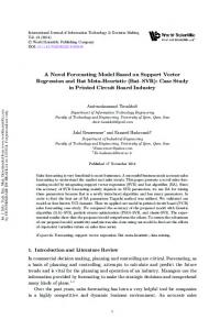
3) DATA SOURCES FOR TRANSIT NETWORK CREATION In this section a brief explanation of all the data sources is given, focusing on the particular purpose of each source and the reasons to use them in DVRPC’s TIM 2.0 network model. A more detailed explanation of the data sources other than Google Transit Feeds is given in a previous paper (1). 3.1) Data Requirements and Reasons for Selecting Web Based Data Specific requirements were established for data sources when DVRPC began the process of building a new network model. The network data must be geographically accurate and the street network must be routable. Transit service data need to be accurate, reliable and provide regular updates. DVRPC decided to use OSM and GTFS datasets for the TIM 2.0 network model based on these requirements (1). Both datasets are freely available on the web without copy right restrictions. 3.2) TIM 2.0 Data Sources The TIM 2.0 model integrates highway and transit network information in one data set. The network geography is shown in Figure 1. DVRPC has used the following data sources for the different network layers:  OSM is the main source for highway network data. This is augmented by data from two of DVRPC’s member counties who provided routable street centerline files. The highway network data primarily consists of nodes and links.  For the transit network, GTFS is the source for lines, service patterns, individual vehicle journeys, and transit stops at a GPS level of detail. The GTFS & OSM data is not sufficient for detailed forecasting needs. Significant elements of additional data are required to produce a useful travel forecasting network, including:  Traffic Analysis Zones (TAZs) and connectors integrate the network model with the travel demand model.  Additions to the transit network include:  a classification and organization of the stop points in a 3-level stop model,  transfers and walking times,  a representation of walk access and auto access,  a computerized representation of the Philadelphia region’s complex fare system,  passenger counts for calibration. 4) THE DATA INTEGRATION PROCESS GTFS data are originally prepared to provide passenger travel information. To integrate these data with a travel model, DVRPC developed a process that balances the operational detail of GTFS on the one hand and the requirements of the travel modeling platform on the other. The process of integration can be divided in three major steps: 1. Translation of GTFS into the model format 2. Merge of the GTFS stops and routes with the OSM derived highway network 3. Transit data enhancements, including: stop organization, transfers, access by walk and auto, fare coding, calibration of path building, and path choice.


5

Source: DVRPC, © in parts OpenStreetMap and CC-BY-SA, and by SEPTA, NJ Transit

FIGURE 1 Regional Network Model Based on OSM and GTFS.

4.1) Translation of GTFS Data into Model Format The import of Google Transit Feed data into the model systems starts with downloading the raw GTFS text data from each operator’s internet site. The data are then translated into the modeling software format. In DVRPC’s case, the modeling software package provides an automated GTFS importer, which filters a GTFS data set for one specific calendar day and then translates the result into the package’s proprietary format. For each schedule update, DVRPC carefully defines this calendar day to represent the average weekday service, typically by selecting a Tuesday or Thursday during a time of the year when secondary schools are open and when no public holiday occurs in the same week. Running the import routine for each operator creates several sub-networks in travel model format. In rare cases, manual modification of the imported schedules is necessary. An example is the modification of temporary schedules, such as when rail service is replaced by a bus during construction projects. In this case the schedule will be replaced with the permanent service from a previous GTFS feed before construction. To be able to consolidate the imported results from all operators into one transit network, the IDs of stops, routes and service trips need to be unique over all sources. To obtain unique IDs, all stops and some routes are systematically renumbered and renamed, while keeping reference to the original IDs used by the operators. DVRPC staff has programmed Python scripts that perform the renumbering and renaming and other post-processing steps such as classification of transit service lines into bus and rail submodes, cleaning of unused stop and route IDs etc.


6

Quality control procedures were used to ensure data quality. DVRPC staff compared the import results extensively with printed schedules while the process was being developed. All errors were used to improve the automated importer as well as the customized post-processing routines. Many sources of errors could be eliminated in cooperation with the transit agencies and the software provider. The import process is now robust and stable with minimal translation errors. The result of the import is a very detailed transit network. Table 1 shows the increased detail for DVRPC’s GTFS-based model (dubbed “TIM 2.0”) as compared to DVRPC’s legacy travel model (“TIM 1.0”) with its coarser representation of the same transit system. The number of stop points is three times higher and the number of service patterns is six times higher. The increased detail is typical for operations data. In the following two sections it will be explained how this increased level of detail was accommodated in the travel model. TABLE 1 Quantitative Comparisons of the Legacy and the GTFS-Based Models Network Statistics* Number of links **

TIM 1.0 Legacy Model

TIM 2.0 - GTFS-based

45,000

496,000

Number of traffic analysis zones

1,900

3,200

Number of transit stop points

5,200

17,500

Number of transit stop areas

5,200

10,800

Number of transit service patterns

1,700

10,300

*: To properly compare with the legacy model, only the network objects inside of the DVRPC region are counted. **: Counting all link directions that are open to at least one highway or transit mode

4.2) Merge with the Street Network Model The transit network needs to be integrated with the street network to allow for the analysis of the interaction between transit vehicles and cars. To integrate GTFS with the street network, a sophisticated data model is needed, which is shown as Entity-Relationship (ER) chart in figure 2. Before integration, the data entities within GTFS are related and organized (green color in the chart) but they do not yet have any relationship with the street-network (blue color). The integration of the transit and street network can be understood as creating new (red) relationships between the green and the blue entities. This concept is described in more detail in a previous paper on this model (1). The integration of the transit with highway networks includes the following tasks: 1. Snapping of stop points onto the street network: This step can be largely automated with intelligent GIS processing, but depending on the quality of stop geo-referencing in the GTFS data, a degree of manual adjustments are required to complete the task. 2. Adjustment of bus route alignments over nodes and links: During the GTFS import, the modeling software proposes a path for routes from one stop to the next one over the link network. However, the bus routing between stop points proposed by the importer does not always match the actual alignment driven by the buses. In these cases the path alignment needs to be corrected.


7

3. Correction of errors in street connectivity and directionality: In the highway network based on OSM and GIS data sources, there are errors in the original data source that prevent a bus route from completing their path. Examples of such errors are missing streets, disconnected links, or errors in one-way direction. These also need to be correct in order to assure proper bus routing. These corrections are beneficial not only for transit integration but for the highway model as well. It is important to note that the extensive data processing of transit-street integration needs to be conducted only for the initial model development. For schedule updates into an existing GTFSbased model, most stops remain unchanged so that stop snapping is minimal and route adjustment will be highly automated. Connector

Zone

Zone Number Node Number Direction

Zone Number

Travel Demand Data Node Number

Stop Area Number Legend 1 or more

2 0 or more Exactly 1

Link From Node To Node

Stop Point Number

from OSM

from GTFS

Line Name

Service Pattern

Scheduled Run

Line Name Route Name Direction

Line Name Route Name Direction Index

Source: DVRPC, first published in (1), based on VISUM data model (5).

FIGURE 2 Simplified Entity-Relationship Chart for the Network Data Model.


8

4.3) Transit Data Enhancements After GTFS import and integration with the street network, complementary information is added that does not originate from GTFS, but is important to complete the transit network. This information includes the organization of stops, transfers, walk access and fare. 4.3.1) Stop Organization and Creation of Transfer Opportunities An important method of dealing with the high level of detail in operational data such as GTFS is to organize the stops. In the DVRPC model stops are coded with a three-level hierarchy. One stop can include several stop areas, while each of the stop areas can include several stop points:  The stop point is the lowest level and represents the geographic location where a transit vehicle physically makes its stop.  The stop area is a grouping of individuals stop points. For example, Both the east-bound and west-bound stops points of a particular bus at a particular intersection are grouped together as a single stop area. This organization is needed to model access to and from zones and to structure transfers within a stop.  The stop is the highest and most abstract data level. It allows to model transfers between different services. In the case of a large station of transit center, a stop can include many stop areas. The stop points in the DVRPC model are a one-to-one match of the GTFS stop data. The stop areas and stops, however, do not come from GTFS but are created by DVRPC to structure the highly detailed GTFS data. There are currently about 11900 stops, 12200 stop areas, and 21400 stop points in the TIM 2.0 model (Table 1).


9

Source: DVRPC, SEPTA, NJ Transit, © in parts Open StreetMap, CC-BY-SA

FIGURE 3 Stop Organization for 30th-Street-Station, Philadelphia, PA. The example of 30th Street Station in Philadelphia (Figure 3) illustrates the three–level stop organization: 13 different transit stop points are reported in GTFS. The 7 bus stop points are consolidated into 3 stop areas. Less consolidation was necessary for rail services, which were aggregated into 4 rail stop areas (SEPTA Regional Rail (RR), Amtrak, NJT, SEPTA Subway, and SEPTA Trolley). In total, the 30th Street Station stop is modeled with 7 stop areas. Assumptions for transfers and walk access only need to be modeled for these 7 stop areas. The relations between the 7 stop areas are populated with walk times and stored as a 7x7 matrix in the network model. 4.3.2) Zone Connectors for Walk Access Transit connectors allow for walk access from TAZs to the transit network via nodes and stop areas (see Figure 2). A TAZ should typically have several connectors, so that there is access to all the different bus and rail routes that serve the zone. The following catchment areas are used for different types of stop areas:  up to 0.25 miles for bus and trolley stops;  up to 0.5 miles for rail stops (RR, Subway, LRT) and end-of the route bus stops;  up to 0.75 miles for the major regional transit hubs.


10

The maximal catchment radius of a stop area is approximate and is not equal to the length of the connector. Important is that all zones that overlap with the catchment area are connected. The catchment radii are approximate. 4.3.3) Walk Times for Access and Transfer DVRPC staff conducted a survey to get a better estimate of the walk times for transfers and transit access by measuring real-world walk times on major rail hubs in the region. One lesson learned is that the assumed walk times in previous DVRPC models were lower than those observed in the survey. The survey showed that important factors of walk time include delays caused by stairs, doors, turnstiles, and also the pedestrian congestion that occurs when many passengers alight large trains at the same time. A linear model was estimated that explains the walk time with information available to the network model: Walk time = 30 sec + MDIS / 3.1 MPH + Delay(From Stop Area) + Delay(To Stop Area) Where:  MDIS = Manhattan distance between the starting stop area and the ending stop area  Delay for stop areas: o 35 sec for major rail station o 20 sec for any other rail stop area o 0 sec for bus stop areas The average error of this walk time model is 29% for observed walk times. The formula is applied for transfer walk times and access times on zone-connectors and has been implemented as a Python script. 4.3.4) Modeling of Fare Each operator in the DVRPC region has its own fare collection and pricing structure. The two largest operators have also different fare structures for some of their sub-divisions. The resulting fare system as a whole is complex with a large set of rules and exceptions. While the GTFS format allows the inclusion of fare information, the transit agencies in the DVRPC region do not yet supply the complete fare information in their GTFS feeds. As such, DVRPC has spent significant effort in researching and coding transit fare for the entire region to allow for a realistic estimate of the fare for each path taken in the model. The approach is based on the new fare modeling framework in VISUM 11.5 (5). As a complete description of DVRPC’s fare modeling would exceed the scope of this paper, only the main principles are given in relationship with GTFS. The most important components of the fare model implementation are:  Fare zones: a fare zone is a set of stops. Each stop needs to be member of at least one fare zone, but can also belong to several fare zones (e.g. for stops at the fare zone border of for hubs with services from many operators).


  

11

Fare systems: a fare system is a set of transit lines. The DVRCP model uses 14 fare systems, where the SEPTA service is divided into 3 fare systems, NJ Transit into 6 fare systems, and five fare systems are defined for the remaining services. Fare rules: within each fare system, there is a zone-based pricing structure that can be given as a matrix from-fare-zone/to-fare-zone or simply dependant on the number of traversed fare zones. Transfer fees between fare systems: if a path includes a transfer from one fare systems to another, additional fees or discounts are defined.

A significant modeling decision has been to avoid any fare coding on links and route segments. Instead, all fare rules are based only on fare zones and fare systems. As a result, the fare model is completely independent of any network coding on nodes, links, routes, and schedules. More important, the fare model will not be affected by an update of the GTFS data. Manual update of fare data in the model is only required if new stops or lines are added to the network. Figure 4 represents the complex fare system in one portion of the region (NJ). Color changes indicate a change in fare zone (FZ) and hence a change in fare. Stops are assigned to their corresponding fare zone numbers and are color coded based on their FZ numbers. For example, NJT’s regional rail has its own fare structure, while NJT bus has a different fare structure. In TIM 2.0 several major transit hubs have been identified where there are different modes and operators at the same location, e.g. 30th Street Station (discussed in 4.3.1 section). These major transit hub stops are assigned to many fare zones because they have different modes of transit, each with a different fare structure.


12

Source: DVRPC, SEPTA, NJ Transit, © in parts Open StreetMap, CC-BY-SA

FIGURE 4 Fare Modeling for DVRPC’s New Jersey Area. 4.3.5) Validation with Transit Passenger Assignments After going through the entire process of data integration and enhancement, the data model has been tested during the calibration of path building and path choice, which is described in the next chapter. Path choice validation helps to discover data errors and network coding problems. For example, if path choice results show that certain transfer opportunities are missing, the assumptions in stop organization are reviewed. 5) ASSIGNMENT METHOD Transit assignment is the process of determining which transit routes/operating patterns passengers will choose over a network to get from their origin to their destination. The related process of skimming determines travel times, costs, and other elements of disutility over these paths. Transit assignment is important for determining link and line volumes. The computer representation of the transit network, in this case developed from GTFS, is the primary input to the assignment and skimming processes. DVRPC’s TIM 2.0 model uses a schedule-based assignment method for transit trips which use walk as their primary mode of access. Trips that


13

use automobiles as their primary mode of access (i.e. Park and Ride) use a combination of the highway and transit network skim results. 5.1) Timetable based Path Choice Transit passenger assignment methods can be grouped into “headway-based” and “schedulebased” categories. The academic literature is rich in work based on either method (12,10), but the majority of travel models use only headway-based assignments, either shortest-path based or multi-path based (8,11). The VISUM software provides a schedule based method, called the “timetable-based assignment” which is applied in this model (9,5). It assumes that the operations schedule is sufficiently reliable, and as a result vehicle and train runs are considered deterministic. The schedule is a detailed data set of the departure and arrival times for each vehicle run in the network. In the case of the TIM 2.0 model, all of this information comes from the GTFS-based transit network. The path builder uses the schedule to build a search graph and finds connections with a branchand-bound approach. Schedule-based assignment is naturally a time-dynamic method, as the time-component is explicitly incorporated in path-building and in path choice. Also, transport supply and conditions of travel vary during the day. Travel supply can be evaluated and skim matrices can be computed exactly for different times of day (9,12). Choice models are used to determine ridership flows between alternative paths and connections. The TIM 2.0 model initially used a Box-Cox transformed logit model, but transitioned to a straight logit model in order to maintain consistency between the path and the mode choice models in TIM 2.0. The impedance or utility includes in-vehicle time, several out-of-vehicle components, a penalty for the difference between desired and effective departure time, and a correction term for similarity of paths. 5.2) Park and Ride Modeling The TIM 2.0 model uses a matrix convolution method to model transit trips with use the automobile to access the first station, also known as park and ride trips. Three pieces of data go into the matrix convolution procedure: 1. A skim matrix of highway travel times/impedance 2. A skim matrix of transit travel times/impedance 3. A designation of certain zones as park-and-ride zones The matrix convolution method examines these two matrices for every ij pair. In this example “i” is the origin zone where the individual starts the trip in an automobile and “j” is the destination zone where the person arrives after taking transit). The method examines all possible park and ride zones “k” where the transfer between auto and transit can take place so that some measure of total auto + transit impedance is minimized. This includes the ik auto portion of the trip from the highway skim matrix and the kj transit portion of the trip from the transit skim matrix. After the optimal park and ride zone “k” is identified, the transit auto-access demand matrix is split into two parts. The ik auto portion is added to the total highway demand matrix for assignment. This way the effect of large park and ride lots on local congestion and on system


14

level metrics (VMT, GHG, etc.) is captured. The kj transit portion of the trip is then assigned to the transit network along with the transit-walk matrix.

6) RESULTS 6.1) Passenger Assignment Results of the transit assignment are shown in Figure 5. Initial assignments before in–depth calibration shows a promising goodness-of-fit with a coefficient of determination of 0.94 for the 24-H boardings per line. Major choices between routes and modes are well represented, even in Philadelphia which has a very dense transit network

Source: DVRPC, © in parts Open StreetMap, CC-BY-SA, SEPTA, NJ Transit

FIGURE 5 Passenger Volumes as Transit Assignment Result. 6.2) Use of the GTFS for Planning Applications The enhancements in the transit network not only serve the purpose of better forecasting results, but are also useful for other planning applications. The GTFS derived TIM 2.0 model has been useful in visualizing & analyzing these already existing data sources. Useful planning applications have included transit frequency, isochrone analysis, average transit speed, and number of buses per day/hour on a particular roadway segment; this secondary data extracted


15

from the posted operation GTFS data is being used by planners and non modelers for corridor as well as regional level planning. The isochrone in Figure 6 shows travel time contours based on GTFS starting at 30th-StreetStation in Philadelphia. The isochrone has been computed by using all transit services that depart between 9:00 and 9:30 AM from the start location, following the shortest path through the entire network. Such evaluations have been conducted for several urban and suburban locations. The results show that accessibility by transit depends strongly on location. Locations like Center City Philadelphia provide much better accessibility by transit compare to suburban locations. This kind of travel time analysis based on operational schedules is possible with the GTFS-based model.

Source: DVRPC, © in parts Open StreetMap, CC-BY-SA, SEPTA, NJ Transit

FIGURE 6 Travel Time Isochrone Starting at City Hall, Philadelphia, PA.


16

7) RESOURCE REQUIREMENTS DVRPC predominantly used internal staff to construct the TIM 2.0 GTFS transit network. While it is difficult to separate the work between the highway network and transit network development, approximately 19 staff-months of time were required to produce the new transit network. Of these 19 months of effort, 70% was from full time staff, while 30% of the effort was simple enough to be performed by interns. It is important to state that these staff resources were needed only for the initial network model development. As tests have shown, the effort for a schedule update will be in the order of magnitude of between one or two man months for the entire network. Details of the staff effort are shown in Table 2. TABLE 2 Resource requirements by task for development of GTFS transit network. Task Process GTFS Data Highway - Transit Integration Transit transfers & fare system calibration, transit assignment

Staff-Months

% Full-time

% Intern

1.0 7.6 5.0 5.6

80% 48% 82% 86%

20% 52% 18% 14%

19.2

70%

30%

8) CONCLUSIONS AND RECOMMENDATIONS DVRPC has successfully processed GTFS data to describe transit service in the Greater Philadelphia regional travel forecasting model. The greatest benefit associated with the use of GTFS is that no manual data entry based on paper-published schedules is required to update the model, as the import of GTFS is highly automated. Moreover, GTFS has been adopted by the majority of transit operators for periodic updates and as a result one common format can be used for all transit service in the region. Data quality has been improved as the previous practice of updating based on paper-published schedules produced errors. The GTFS transit network also covers all 24 hours of the day, which allows the automatic determination of specific differences in services during the day, e.g. between morning peak, afternoon peak, midday, evening and night. The detailed operational data in the GTFS is augmented by other relevant data including improved representations of walk times, transfers, fare. A more accurate treatment of the interaction between highway travel and public transportation is also contained in the new transit model (Park&Ride, capacity and speed effects on shares streets). The GTFS transit network, in providing an integrated and readily accessible database of all transit services in the region, has proven to be valuable for planning applications that do not involve travel modeling or forecasting. In this way, the GTFS network is able to provide analysis and insight into already existing data. Most likely, GTFS can also be a useful resource for government agencies and transportation consultants in other regions. An important condition is certainly the advancement of Google Feeds in the particular region of interest. In the long run, the authors are convinced that coverage and data quality of internet-based transportation data will increase and as a result there will be more and more opportunities for government applications.


17

ACKNOWLEDGEMENTS We thank Matthew Gates, Greg Burton, Klaus Nökel and Chetan Joshi for their contributions to the network model development. REFERENCES 1. Scherr, W., G. Burton and C. Puchalsky. A Paradigm Shift in Travel Forecasting: Let Web 2.0 Feed the Network Model. Paper presented at 89th Annual Meeting of the Transportation Research Board, Washington, D.C., 2010. 2. General Transit Feed Specification. Information for Riders, Developers and Transit Agencies. http://code.google.com/transit/spec/transit_feed_specification.html. Accessed July 24, 2010. 3. TriMet. Transit Investment Plan. http://trimet.org/pdfs/tip/tip.pdf. Accessed on July, 25, 2010. 4. GTFS Exchange Site. http://www.gtfs-data-exchange.com. Accessed on July, 25, 2010. 5. VISUM 11.5 Manual. PTV AG, Karlsruhe, Germany, 2010. 6. Goodchild, M. Citizens as Voluntary Sensors: Spatial Data Infrastructure in the World of Web 2.0. International Journal of Spatial Data Infrastructures Research, Vol. 2, 2007, pp. 24-32. 7. Open Street Map. Beginner’s Guide, Press Room. http://wiki.openstreetmap.org. Accessed July 24, 2010. 8. Fisher, I., K. Lew, W. Scherr and C. Xiong. Planning of Vancouver’s Transit Network with an Operations-Based Model. Paper presented at 55th North American Meeting of the Regional Science Association International. New York, NY, Nov. 2008. 9. Friedrich, M., I. Hofsaess and S. Wekeck (2001): Timetable-Based Transit Assignment Using Branch and Bound. TRB Annual Meeting, Washington D.C. 10. Nuzzolo, A. (2003): Schedule-Based Transit Assignment Models. In: Lam, W. and M. Bell: Advanced Modelling for Transit Operations and Service Planning. Pergamon, Oxford, UK. 11. Kurth, D., S. Childress, E. Sabina, S. Ande, L. Cryer (2008): Transit Path Building. To Multipath or Not to Multipath. Transportation Research Record: Journal of the Transportation research Board, No. 2077, pp.122-128, National Academies, Washington D.C. 12. Hamdouch, Y., Lawphongpanich, S., (2008): Schedule-based Transit Assignment Model with Travel Strategies and Capacity Constraints. Transportation Research Part B: Volume-42 Issue Number 7-8, pp. 663-684, National Academies, Washington D.C.