BUIlLDING A REGIONAL FORECASTING MODEL UTaIZING LONG-TERM RELATIONSIllPS AND SHOR17-TERM INDICATORS Keith R. Phillips
and Chih-Ping Chang
June 1995
RESEARCH DEPARTMENT WORKING PAPER 95-04
Federal Reserve Bank of Dallas This publication was digitized and made available by the Federal Reserve Bank of Dallas' Historical Library (
[email protected])
Building a Regional Forecasting Model Utilizing Long-term Relationships and Short-term Indicators'
Keith R Phillips Federal Reserve Bank of Dallas
Chili-Ping Chang Southern Methodist University
June 1995
'The authors thank seminar participants of the November 1994 Federal Reserve Regional System Committee Meeting and Nathan S. Balke for helpful comments. The views expressed in this paper are those of the authors and should not be attributed to the Federal Reserve Bank of Dallas or the Federal Reserve System.
Abstract
Chang and Phillips develop a simple labor-demand error correction model of regional employment growth. The model is constructed to forecast well at both long-term and short-term horizons. In developing the model, we utilize past research which has found that relative nominal wages play an important role in explaining why some regions consistently grow faster than others. The variables in the model include regional employment,
u.s. employment, an
industry-adjusted relative wage measure, and a regional leading index. While the wage variable is used to capture long-term shifts in relative labor demand, the leading index is included to control for shorter-term cyclical shocks. Out-of-sample forecast errors from the model are shown to be smaller than errors from a model suggested by LeSage (1990a) which divides regional employment into base and nonbase and estimates a bivariate error-correction model.
I. Introduction
Regional economists are often asked to produce forecasts that range anywhere from several months to several years. Often, however, the forecasting technique and variables used by the analyst differ depending on whether the forecast is long- or short-term. For example, the analyst might use average weekly hours of manufacturing workers to forecast short-term cyclical movements in regional employment but would not likely use the same indicator for forecasting longer-term changes. In this article we attempt to build a simple regional forecasting model that utilizes short-term indicators and long-term relationships in an attempt to forecast well at both short-term and long-term forecasting horizons. In a recent series of articles, LeSage (1990a, b) and Shoesmith (1995) developed several error-correction models to forecast regional employment. The purpose of the error-correction model is to determine and estimate any long-term equilibrium relationships that exist among nonstationary variables. Given that these stationary relationships can be established, using the Error-Correction Vector-Autoregressive Model (ECM) has more appeal than simply running models in first-differenced form and thus focusing on the short-term relationship between the variables. In this article we develop an ECM which utilizes the long-term equilibrium relationship between a region's relative employment and its relative wage. (The term relative refers to relative to the national average, unless stated otherwise.) The model also utilizes movements in a regional leading index in an attempt to capture upcoming short-term cyclical shocks. We develop a four-variable ECM for the Texas economy and compute out-of-sample forecasts between March 1991 and March 1995 and for the 1986 Texas recession. Errors from one- to thirty-six-step ahead forecasts are compared to a two-variable ECM suggested by LeSage (1990a) which divides employment into base and nonbase. Our model performs better on
1
average during each forecasting period and at almost all forecast horizons within each period. The results suggest that our model may be useful for forecasting total nonagricultural employment at the regional level.
II. Developing a Regional Forecasting Model
In an attempt to forecast employment for fifty different industries in Ohio, LeSage (1990b) finds significant cointegration between manhours, hourly earnings, and the consumer price index in seven industries. He then compares out-of-sample errors from an ECM for each of the fifty industries to errors from a differenced Vector-Autoregressive Model (VAR), two types of Bayesian VARs and a Bayesian ECM. In the seven industries with cointegration, he finds that the ECM performs best. He also finds, however, that the ECM performed well at the seven- to twelve-month forecast horizons, even in models that failed the cointegration tests. In another paper, LeSage (1990a) forecasts total nonfarm employment for eight different metropolitan areas in Ohio using the ECM within the context of the economic base model. Using the three categories of durable, nondurable, and nonrnanufacturing industries, LeSage defines base employment during any month as any positive residual of employment in an industry minus what the
u.s. industry share would suggest.
After dividing employment into base
and nonbase, he finds evidence of cointegration between the two employment types in each of the eight cities. He then compares the results of the ECM to the four types of models described in LeSage (1990b) and to a forecast produced by an independent analyst. LeSage finds that the ECM and BECM used in the context of a dynamic economic base model performed the best out of the six models examined and concludes that the ECM used on base and nonbase employment was a simple, but effective, way to forecast regional employment. The results of the two LeSage articles give strong evidence of the usefulness of the ECM
2
in forecasting regional employment. The use of the economic base model, however, is less convincing. Although the economic base model has a long history in regional economics, in recent years it has faced increasing criticism.' While the LeSage results give evidence that base and nonbase industries share a long-term relationship and that growth in base industries leads to growth in nonbase industries, it may be possible to construct a simple regional ECM that has stronger links to regional employment growth. The use of the ECM in regional forecasting is based on finding variables that share a long-term cointegrating relationship. Finding variables that share this type of relationship may often be difficult. For example, Hefner (1990) showed that for all eight Bureau of Economic Analysis regions, Gross State Product was not cointegrated with U.S. Gross Domestic Product, and Shoesmith (1992) showed that for every state except Vermont, U.S. nonfarm employment was not cointegrated with the state nonfarm employment. Shoesmith (1995) also showed that in his five-variable regional VAR model, ouly one out of four states tested had at least one significant cointegrating vector. These results emphasize the need for a strong theoretical notion of what variables are likely to experience stable long-term relationships. One stylized fact important in long-run regional employment forecasting is that many regions consistently grow faster than others. Browne, Mieszkowski, and Syron (1980) in a study of the relative economic strength of the South, found that low nominal wages played an important role in attracting net investment into the South. Using surveys, other researcherssuch as Nakosteen and Zimmer (1987) and Wheat (1986)-have confirmed the importance of relative nominal wages in regional job growth. Kottman (1992) suggested that, for industries which export nationally, the decision on where to produce is a function of relative nominal wages, but for workers the decision on where
'For a good summary of the recent criticisms of the economic base mode~ see Krikelas (1992).
3
to work is a function of relative cost-of-living adjusted wages. Kottman points out that in terms of labor supply, "There is an emerging consensus in the literature that regional wage and income differentials have all but vanished once adjusted for cost-of-living and labor force characteristics." He concludes that the persistent migration of capital and labor appears to be almost solely due to labor demand - firms migrate to areas with low relative nominal wages. While workers' real wages are similar across regions, low nominal wages stimulate relatively strong job growth. In our model, we adopt the view that the main factor driving relative regional employment growth is shifting labor demand which is driven mainly by relative nominal wages. As information flows into the high-wage regions and firms realize that they can increase profitability by moving to low-wage regions, firms begin to migrate. As firms migrate to the lowwage regions they build up the regional infrastructure, which motivates more firms to move in gradually shifting out the labor demand curve in the low-wage regions. In the traditional labormarket model, shifts in labor demand result in a positive relationship between employment and real wages as the labor supply curve is upward sloping. In this
mode~
low-wage regions
experience relatively strong labor demand shifts, which result in stronger gains in wages and employment than in high-wage regions.' Thus, we expect a positive long-run relationship between a region's relative wage and its relative employment. An industry is attracted to a region if wages in that region are relatively low. It is thus important to compare wages across the same industry and not just compare total manufacturing wages. We thus create a wage variable which measures the percentage difference in an industry's wage from the same industry in the nation at the two-digit Standard Industrial
'One implication of this model is that wages in the low-wage region would be driven up while wages in the high-wage region would be driven down - leading to wage convergence. Supporting this notion, Carlino and Mills (1993) find statistical evidence that per capita incomes have converged in the United States since 1929, and Browne (1989) points out that most of the movement in per capita personal income-at least over the past two decades-has been due to variations in wages.
4
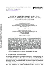
Classification level. The wage differentials are weighted together by the industry's share of national manufacturing employment to form a composite measure of the region's relative manufacturing wage. Chart 1 shows that in Texas this wage measure appears to share a longterm positive relationship with Texas nonfarm employment. While we expect a long-term relationship between relative wages and relative employment, we also expect employment to exhibit business-cycle patterns because of economic shocks such as oil price changes. To incorporate these short-term shocks, we include the Texas Leading Index which was designed to predict cyclical turning points in the state's economy.' The components of the Texas Leading Index are average weekly hours of production workers in manufacturing, an index of help-wanted advertising, an index of stock prices of companies based in Texas, new unemployment claims (inverted), real retail sales, permits to drill oil and gas wells, the real price of crude oil, the BEA national leading index, and an index of the real exchange rate of the countries Texas exports to (inverted). Phillips (1988, 1990) has shown the index to be a reliable indicator of turning points in the Texas economy with a lead time of three to eight months. The long-run relationship suggested by the labor demand model is
(RW)
where In is the natural log function, TXEMP and USEMP are the levels of nonfarm employment in Texas and the United States, and RW is a measure of Texas hourly wages relative to U.S. hourly wages. Preliminary testing showed that a significant long-term
'The use of regional leading indexes has proliferated over the past ten years. For a description of the typical index calculation and a listing of indexes available at the regional level, see Phillips (1994). For more information on the components in and the calculation of the Texas Leading Index, see Phillips (1990).
5
relationship holds between the two variables in this equation.s While this relationship is important in forecasting the relative growth of Texas employment in the long-run, it is also likely that changes in the Texas Leading Index (TXLI) are important in directly predicting shorterterm cyclical shocks to the Texas economy. However, since the TXLI is not likely to have proportional effects on both TXEMP and USEMP, we build the model based on the relationship between all four variables. The four-equation ECM we estimate is
ax,
= JL
+A(L ).6.X,_, +a~X;_k_1 +e,
where X, is a vector containing four series - Texas' relative wage (rw), the Texas Leading Index
(txli), Texas nonfarm employment (txemp), and U.S. nonfarm employment (usemp) - and
A
is
the first-difference operator. The lowercase of a variable indicates its logarithmic value. A(L) is a lag polynomial of order k.
~X
is the error-correction term capturing the stationary long-run
equilibrium among the four variables. For example, the equation of Texas nonfarm employment in the VAR model is specified as T
T
T
T
Attemp,=1-l + I: A/Attempt-/+ I: 6/"rwt-/+ I: y/"txlit-/+ I: TJ,,,usemp,_/ i=1
i=1
1"'1
1=1
+Cl(~lrw+~ixli+~3ttemp+~4usemp)'_T_l +e,
where T is the number of lags and the term in the parentheses specifies the cointegrating relationship.
III. Data
'The Johansen and Juselius (1990) cointegration test was run for these two variables over the sample of 74:1 to 91:2 with the VAR lag length of 6. We did find one significant cointegrating vector at the 5 percent level. The stationary long-run relationship between relative employment and relative wage implies that the two series should not move too far apart. Any divergence from the equilibrium should be considered temporary.
6
The variables used to estimate the model are Texas nonfarm and U.S. nonfarm employment, TXLI, and the Texas manufacturing wage relative to the U.S. manufacturing wage. As described earlier, we construct a measure of relative wages that adjusts for the differing industrial structure in the region than in the nation. The wage variable is intended to measure the relative wage across industries that is due solely to wage differences and not to differences in industrial structure. The relative wage variable is calculated as follows:
where RW, is the relative wage, HWTX;, is the hourly wage in industry i in Texas, HWUS" is the hourly wage in industry i in the U.S., EUS. is U.S. employment in industry i, and EUS, is U.S. manufacturing employment summed across nineteen two-digit manufacturing industries available at both the state and national levels and t is a time SUbscript'. Thus the wage variable is constructed by calculating relative wages at the two-digit manufacturing level and weighting each industry's relative wage by the industry's U.S. employment share. The wage and employment data are from the Current Employment Statistics (CBS) series produced by the Bureau of Labor Statistics. In order to compare our model to the model developed by LeSage (1990a), we calculate base employment in Texas with the following formula by LeSage: EUSu RNEu=RE,(--) EUS,
where RNE. is the number of employees in industry i that is necessary to supply local needs,
REt is total regional employment, EUS. is U.S. employment in industry i and EUS t is total U.S.
'Por Texas, wages for nineteen of the twenty two-digit manufacturing industries were available during this time period. At the nationalleve!, wages for Electric and Electronic Equipment, and Instruments and Related Products did not begin unti11988, and so altogether seventeen of the twenty industries were used.
7
employment. If RNE" is greater than or equal to
RE", nonbase employment in industry i is then
equal to RE" and base employment in industry i is equal to zero. If RNE" is less than RE", then local employment in industry i is equal to RNE" and base employment is equal to RE" minus
The dynamic location quotient described above generates two time-series data which represent monthly magnitudes of local (nonbasic), denoted by LE, and export (basic) employment, denoted by XE, for the state of Texas. While LeSage used employment data in only three categories - durable, nondurable, and nonmanufacturing employment - we include employment at the two-digit SIC level in manufacturing and at the division level in nonmanufacturing, for a total of twenty-nine industries. The nonfarm employment data for different sectors in Texas are from the CBS. The data are seasonally adjusted with the adjustment procedure described in Berger and Phillips (1993, 1994). This adjustment controls for a break in the seasonal pattern which is often found in the state employment data.
IV. Econometric Methodology
Applying conventional VAR techniques will lead to spurious results if the variables in the system are nonstationary. The mean and variance of a nonstationary, or integrated, time series which has a stochastic trend, will depend on time. Any shock to the variable will have permanent effects on it. The most common procedure to render the series stationary is to transform it into first differences. Nevertheless, the model in first differences will be misspecified if the series are cointegrated and converge to stationary log-term equilibrium relationships.7 The set of variables
7The concept of cointegration, first proposed in Granger and Weiss (1983), is fundamental to the use of the error-correction-model formulation. Engel and Granger (1987) have shown that a model estimated using differenced data will be misspecified if the variables are cointegrated and the cointegrating relationship is ignored. Cointegration means that nonstationary time series variables tend to move together such that a linear combination of them is stationary. Cointegration is sometimes interpreted as representing a long-run
8
in the system must cointegrate for a valid Error-Correction VAR (ECM) to exist. Therefore, tests for cointegration should be a necessary component of estimation exercises conducted with ECMs. In our analysis we test for cointegration using the general maximum likelihood approach of Johansen and Juselius (11) (1990). The 11 approach differs from Engel and Granger (1987)8, which LeSage (1990a) adopts, in that it offers an explicit criterion for choosing the number of cointegrating vectors. Suppose
X, is a (pxl) vector of first difference stationary time series variables, the ECM form is
where
r, =
-1+ II, + ... +II,
0= 1,...,k-l) and II
=
aW, Wis the (pxr) cointegrating vector, and a is
the (pxr) vector of error correction coefficients (or speed of adjustment). E,
rr. is a pxp matrix and
is a vector with p elements composed of independently and normally distributed random
disturbances with zero means. In 11,
~
can be estimated and Rank(II) can be determined by the trace test and the
maximum eigen-value test. We employ both tests to check the sensitivity of the results. The former tests the null hypothesis that there are at most r cointegrating vectors against a general alternative, and the latter test the null of r cointegrating vectors against the alternative of at least (r+ 1). Notice that if Rank(II) =r=p, any vector is a cointegrating vector and hence all the variables in X, are stationary. If Rank(II)=r.,~(0.95)
>.-
>._(0.95)
r=O
r~ l/r= 1
50.68** 52.89**
47.18
37.98** 39.69**
27.17
r=1
r~2/r=2
12.70 13.20
25.51
5.82 8.24
20.78
r=2
r~3/r=3
6.88 4.97
15.20
5.53 4.91
14.04
r=3
r~4/r=4
1.35 0.05
3.96
1.35 0.05
3.96
Notes: The lag length in VAR is chosen to eliminate the autocorrelation of the residuals in each equation. The upper statistics are for the sample 74:1-91:2, the lower are for the sample 74:1-85:4. Variables included in the test are rw, txli, txemp, and usemp. A model that allows for linear trends is fitted to the data, which results in the cointegrating vectors without a constant term.
LeSage Model, test variables: xe, Ie HyPothesIs
Statistics and Critical Values
Null
Alt.(trace/>.-max)
Atraoe
>.,~(0.90)
>.~
>'~0.90)
r=O
r~l/r=1
18.57* 30.18**
17.96
14.46* 28.51 **
13.78
r=1
r~2/r=2
4.11 1.67
7.56
4.11 1.67
7.56
Notes: The lag length in VAR is chosen to eliminate the autocorrelation of the residuals in each equation. The upper statistics are for the sample 74:1-91:2, the lower one for the sample 74:185:4. Variables included in the test are xe and Ie. * indicates rejection of the null hypothesis at the 10-percent level. ** indicates rejection of the null hypothesis at the 5-percent level.
Table 3: Causality Tests: monthly data 74:1-91:2 I. Panel A: EOUATIONS
i= 1,2,3
MW
Atxli
Atxemp
Ausemp
F(3,188)
F(3,188)
F(3,188)
F(3,188)
2.48*
0.34
1.79
7.98***
3.35**
.6.rw H Atxli,.,
1.15
Atxempt.,
5.04**
0.81
Ausempt_i
2.25*
0.23
1.20
1-4
F(1,188)
F(1,188)
F(1,188)
F(I,188)
EC,.,
13.15***
6.11***
6.23**
4.45**
Q(36)
35.47
36.62
38.93
22.99
0.54
II. Panel B:
i= 1,2,3
1
4
EC,.,
Q(36)
41.04
39.18
Notes: ** *, **, and * indicates significance at the I-percent, 5-percent, and lO-percent levels respectively.
TABLE 4: OUT-OF-SAMPLE FORECASTS Mean Absolute Percentage Errors Chang/Phillips and LeSage Models Horizons
March 91 - March 95
May 85 - May 87
1
0.17(0.16)
0.25(0.30)
4
0.33(0.38)
0.74(1.38)
8
0.52(0.80)
1.83(3.45)
12
0.72(1.32)
3.32(5.55)
16
0.93(1.77)
4.68(6.95)
20
1.15(2.15)
5.30(7.42)
24
1.31(2.62)
5.83(7.58)
28
1.58(3.18)
5.83(7.04)
32
1.73(3.74)
5.65(5.77)
36
1.82(4.26)
5.66(4.97)
Average*
1.05(2.08)
4.08(5.57)
Notes: (1) The numbers in parentheses are for the LeSage base -nonbase model. All values are in percent. (2) The in-sample estimations for both models start from January 1974. *The reported average is the mean of MAPEs for all thirty-six horizons.
CHART 1
o
-2.4
-2
- •• - - • Relative Wage (left seale)
-2.5
- - - Relative Employment (right seale)
-4
.. '.
-2.6
'
-6
..
I'''~.
I
',,- ..
."-:
•• •
~~i'"
,
•
. . .....
" , '
I'
-8
• ••
. ., , ,, ",..,. . ':', .......... I ..... '
"
, "
..,"
..···u..
~
"
.. \
,
....',.." ...
-, ...
"
-10
-12
-2.7
'
. .~ :'" ,.
,~
, ,,
-2.8
",
'"
i
-2.9 -14
-3
-16
71
74
77
80
83
86
89
92
95
RESEARCH PAPERS OF THE RESEARCH DEPARTMENT FEDERAL RESERVE BANK OF DALLAS Available, at no chatge, from the Reseatch Depattment Federal Reserve Bank of Dallas, P. O. Box 655906 Dallas, Texas 75265-5906 Please check the titles of the ReseatCh Papers you would like to receive: 9201 9202 9203 9204 9205 9206 9207 9208 9209 9210 9212 9213 9214 9215 9216 9301 9302 9303 9304 9305 9306 9307 9308 9309 9310 9311 9312
9313 9314 9315
Are Deep Recessions Followed by Strong Recoveries? (Matk A. Wynne and Nathan S. Balke) The Case of the "Missing M2" (John V. Duca) Immigrant Links to the Home Country: Implications for Trade, Welfate and Factor Rewatds (David M. Gould) Does Aggregate Output Have a Unit Root? (Matk A. Wynne) luflation and Its Variability: A Note (Kenneth M. Emery) Budget Constrained Frontier Measures of Fiscal Equality and Efficiency in Schooling (Shawna Grosskopf, Kathy Hayes, Lori L. Taylor, Williatn Weber) The Effects of Credit Availability, Nonbank Competition, and Tax Reform on Bank Consumer Lending (John V. Duca and Bonnie Garrett) On the Future Erosion of the North American Free Trade Agreement (William C. Gruben) Threshold Cointegration (Nathan S. Balke and Thomas B. Fomby) Cointegration and Tests of a Classical Model of Inflation in Argentina, Bolivia, Brazil, Mexico, and Peru (Raul Anibal Feliz and John H. Welch) The Analysis of Fiscal Policy in Neoclassical Models' (Matk Wynne) Measuring the Value of School Quality (Lori Taylor) Forecasting Turning Points: Is a Two-State Chatacterization of the Business Cycle Appropriate? (Kenneth M. Emery & Evan F. Koenig) Energy Security: A Comparison of Protectionist Policies (Mine K. Yiicel and Carol Dahl) An Analysis of the Impact of Two Fiscal Policies on the Behavior of a Dynamic Asset Matket (Gregory W. Huffman) Human Capital Externalities, Trade, and Economic Growth (David Gould and Roy J. Ruffin) The New Face of Latin America: Financial Flows, Matkets, and lustitutions in the 1990s (John Welch) A General Two Sector Model of Endogenous Growth with Human and Physical Capital (Eric Bond, Ping Wang, and Chong K. Yip) The Political Economy of School Reform (S. Grosskopf, K. Hayes, L. Taylor, and W. Weber) Money, Output, and lucome Velocity (Theodore Palivos and Ping Wang) Constructing an Alternative Measure of Changes in Reserve Requirement Ratios (Joseph H. Haslag and Scott E. Hein) Money Demand and Relative Prices During Episodes of Hyperinflation (Ellis W. Tallman and Ping Wang) On Quantity Theory Restrictions and the Signalling Value of the Money Multiplier (Joseph Haslag) The AJgebra of Price Stability (Nathan S. Balke and Kenneth M. Emery) Does It Matter How Monetary Policy is Implemented? (Joseph H. Haslag and Scott Hein) Real Effects of Money and Welfare Costs of luflation in an Endogenously Growing Economy with Transactions Costs (Ping Wang and Chong K. Yip) Borrowing Constraints, Household Debt, and Racial Discrimination in Loan Matkets (John V. Duca and Srnat! Rosenthal) Default Risk, Dollarization, and Currency Substirntion in Mexico (Williatn Gruben and John Welch) Technological Unemployment (W. Michael Cox) Output, luflation, and Stabilization in a Small Open Economy: Evidence from Mexico (John H. Rogers and Ping Wang)
9316 9317 9318 9319 9320 9321 9322 9323" 9324 9325 9326 9327 9328 9329" 9330 9331 9332 9333 9334 9335 9336 9337 9338 9339 9340 9341 9342 9401 9402 9403 9404 9405 9406 9407 9408 9409 9410 9411 9412
Price Stabilization, Output Stabilization and Coordinated Monetary Policy Actions (Joseph H. Haslag) An Alternative Neo-Classical Growth Model with Closed-Form Decision Rules (Gregory W. Huffman) Why the Composite Index of Leading Indicators Doesn't Lead (Evan F. Koenig and Kenneth M. Emery) Allocative Inefficiency and Local Government: Evidence Rejecting the Tiebout Hypothesis (Lori L. Taylor) The Output Effects of Government Consumption: A Note (Mark A. Wynne) Should Bond Funds be Included in M2? (John V. Duca) Recessions and Recoveries in Real Business Cycle Models: Do Real Business Cycle Models Generate Cyclical Behavior? (Mark A. Wynne) Retaliation, Liberalization, and Trade Wars: The Political Economy of Nonstrategic Trade Policy (David M. Gould and Graeme L. Woodbridge) A General Two-Sector Model of Endogenous Growth with Human and Physical Capital: Balanced Growth and Transitional Dynamics (Eric W. Bond, Ping Wang,and Chong K. Yip) Growth and Equity with Endogenous Human Capital: Taiwan's Economic Miracle Revisited (MawLin Lee, Ben-Chieh Liu, and Ping Wang) Clearinghouse Banks and Banknote Over-issue (Scott Freeman) Coal, Natural Gas and Oil Markets after World War II: What's Old, What's New? (Mine K. Yiicel and Shengyi Guo) On the Optimality of Interest-Bearing Reserves in Economies of Overlapping Generations (Scott Freeman and Joseph Haslag) Retaliation, Liberalization, and Trade Wars: The Political Economy of Nonstrategic Trade Policy (David M. Gould and Graerne L. Woodbridge) (Reprint of 9323 in error) On the Existence of Nonoptimal Equilibria in Dynamic Stochastic Economies (Jeremy Greenwood and Gregory W. Huffman) The Credibility and Performance of Unilateral Target Zones: A Comparison of the Mexican and Chilean Cases (Raul A. Feliz and John H. Welch) Endogenous Growth and International Trade (Roy J. Ruffin) Wealth Effects, Heterogeneity and Dynamic Fiscal Policy (Zsolt Becsi) The Inefficiency of Seigniorage from Required Reserves (Scott Freeman) Problems of Testing Fiscal Solvency in High Inflation Economies: Evidence from Argentina, Brazil, and Mexico (John H. Welch) Income Taxes as Reciprocal Tariffs (W. Michael Cox, David M. Gould, and Roy J. Ruffm) Assessing the Economic Cost of Unilateral Oil Conservation (Stephen P.A. Brown and Hillard G. Huntington) Exchange Rate Uncertainty and Economic Growth in Latin America (Darryl McLeod and John H. Welch) Searching for a Stable M2-Demand Equation (Evan F. Koenig) A Survey of Measurement Biases in Price Indexes (Mark A. Wynne and Fiona Sigalla) Are Net Discount Rates Stationary?: Some Further Evidence (Joseph H. Haslag, Michael Nieswiadomy, and D. J. Slottje) On the Fluctuations Induced by Majority Voting (Gregory W. Huffman) Adding Bond Funds to M2 in the P-Star Model of Inflation (Zsolt Becsi and John Duca) Capacity Utilization and the Evolution of Manufacturing Output: A Closer Look at the "BounceBack Effect" (Evan F. Koenig) The Disappearing January Blip and Other State Employment Mysteries (Frank Berger and Keith R. Phillips) Energy Policy: Does it Achieve its Intended Goals? (Mine Yiicel and Shengyi Guo) Protecting Social Interest in Free Invention (Stephen P.A. Brown and William C. Gruben) The Dynamics of Recoveries (Nathan S. Balke and Mark A. Wynne) Fiscal Policy in More General Equilibriium (Jim Dolman and Mark Wynne) On the Political Economy of School Deregnlation (Shawna Grosskopf, Kathy Hayes, Lori Taylor, and William Weber) The Role of Intellectnal Property Rights in Economic Growth (David M. Gould and William C. Gruben) U.S. Banks, Competition, and the Mexican Banking System: How Much Will NAFTA Matter? (William C. Gruben, John H. Welch and Jeffery W. Gunther) Monetary Base Rules: The Currency Caveat (R. W. Hafer, Joseph H. HasIag, andScott E. Hein) The Information Content of the Paper-Bill Spread (Kenneth M. Emery)
9413 9414 9415 9501 9502 9503 9504
The Role of Tax Policy in the BoomlBust Cycle of the Texas Construction Sector (D'Ann Petersen, Keith Phillips and Mine Yiicel) The p* Model of Inflation, Revisited (Evan F. Koenig) The Effects of Monetary Policy in a Model with Reserve Requirements (Joseph H. Haslag) An Equilibrium Analysis of Central Bank Independence and Inflation (Gregory W. Huffman) Inflation and Intermediation in a Model with Endogenous Growth (Joseph H. Haslag) Country-Bashing Tariffs: Do Bilateral Trade Deficits Matter? (W. Michael Cox and Roy J. Ruffin) Building a Regional Forecasting Model Utilizing Long-Term Relationships and Short-Term Indicators (Keith R. Phillips and Chih-Ping Chang)
Name:
Organization:
Address:
City, State and Zip Code:
Please add me to your mailing list to receive future Research Papers:
Yes
- - No
Research Papers Presented at the 1994 Texas Conference on Monetary Economics April 23-24,1994 held at the Federal Reserve Bank of Dallas, Dallas, Texas Available, at no charge, from the Research Department Federal Reserve Bank of Dallas, P. O. Box 655906 Dallas, Texas 75265-5906
Please check the titles of the Research Papers you would like to receive: 1
A Sticky-Price Manifesto (Laurence Ball and N. Gregory Mankiw)
2
Sequential Markets and the Suboptimality of the Friedman Rule (Stephen D. Williamson)
3
Sources of Real Exchange Rate Fluctuations: How Important Are Nominal Shocks? (Richard Clarida and Jordi Gali)
4
On Leading Indicators: Gelling It Straight (Mark A. Thoma and Jo Anna Gray)
5
The Effects of Monetary Policy Shocks: Evidence From the Flow of Funds (Lawrence J. Christiano, Martin Eichenbaum and Charles Evans)
Name:
Organization:
Address:
City t State and Zip Code:
Please add me to your mailing list to receive future Research Papers:
Ves
No