Development Of A Robust Scheduling Rule For A Printed Wiring ...

Development Of A Robust Scheduling Rule For A Printed Wiring Board Drilling Operation With Multiple Scheduling Objectives And Fixed Order Release / Pickup Times Lauren Fowler Department of Mathematics Point Loma Nazarene University San Diego, CA 92106 Michele Pfund, Lian Yu, John W. Fowler, W. Matthew Carlyle Department of Industrial Engineering Arizona State University Tempe, AZ 85287-5906 Abstract We investigate the performance of five approaches to scheduling a Japanese printed wiring board manufacturer’s drilling operation subject to uncertainty. We present and evaluate two optimization approaches against three dispatching heuristics in order to determine how five performance measures are impacted by various levels of processing time variability and equipment breakdowns.

Keywords Scheduling, dispatching, discrete event simulation, variability.

1. Introduction A major goal of the electronics industry is to produce more technologically advanced products at lower prices, while at the same time contending with increasing manufacturing costs for equipment and facilities. Therefore, companies must constantly discover new and improved methods of manufacturing in order to compete in the market place. Efficient dispatching (machine scheduling) is one of the many topics researched by manufacturers. The electronics industry has a wide range of products and companies need their machinery to handle many types of products. Unfortunately, these machines are very expensive and there may be differences in the machines within a single work center. It is difficult to solve the problem of assigning products to appropriate available machines when machines have unique processing times, unique products they can handle, and a number of production goals. This research attempts to improve equipment operations within the bottleneck operation (the drilling center) of a Japanese printed wiring board (PWB) manufacturer. The drilling center contains 14 numerical control machines that have unique processing times for the various products made by the manufacturer. The machines are subject to variability in processing times and can experience small breakdowns or jams. The goal is to design and evaluate approaches that are capable of performing well under uncertainty.

2. Problem Description Multiple machines in a work center are called parallel machines. If the processing times are the same on these machines for any given product, the machines are called identical parallel machines. When the ratio of the time across machines is constant, they are called uniform parallel machines. If the machines are neither identical nor uniform, they are said to be unrelated parallel machines. Most identical and uniform parallel machine scheduling problems are NP-Hard. Manufacturers constantly juggle multiple objectives to find an effective solution that performs well for all objectives. Unfortunately, not all machines have the same processing times and all machines may undergo breakdowns that hinder manufacturing. Variability can have an effect on whether dispatching or optimization approaches should be used. There are higher quality solutions in optimization methods than in dispatching; however, the solutions from the dispatching methods may be better than the optimization solutions when the variability is substantial.

PWB manufacturing consists of many steps. The bottleneck of this particular PWB process is the drilling area. The drilling area is comprised of 14 machines. These machines possibly may not be capable of processing all the different types of lots, but are flexible enough to be able to switch products and still have minimal setup time. Lots arrive to the drilling by an AGV every 3 (T) hours with the number of lots normally distributed with a mean of 30 and a standard deviation of 1.5. Lots that are not completed by T are late and must be delivered by hand to the next station. Management is interested in five performance measures. Each is briefly described below. 1. Makespan - the latest completion time of any job in a release interval. 2. Average Finishing Time - the average time that a machine finishes all jobs in a release interval. 3. Utilization - the percentage of time that the machines are busy. 4. Number of late jobs - the number of jobs completed after the next release of materials (T). 5. Total amount of overtime - the total amount of overtime for all jobs within a release interval. Desired scheduling approaches are those that perform well simultaneously for the five performance measures. We test this using discrete event simulation. Upon completion of each run, the results for each of the measures described above are collected. Upon completion of all simulation replications, the scheduling approaches are compared to each other using the following ranking methodology. Np

CombinedPerformance of SchedulingApproach=

Rp

∑ p =1 R

max

Np

(1)

Rp is the rank of the scheduling approach performance for a specific performance measure, Rmax is the maximum possible rank, and Np is the total number of performance measures under consideration. Given the five scheduling approaches examined in this study, the highest (best) possible rank is 5 and the worst possible rank is 1. Thus a combined performance ranking of 1 indicates that an approach was superior in all five measures, while a value of 0.2 indicates that the particular approach was dominated by the other scheduling methods for all measures.

3. Scheduling / Dispatching Approaches The scheduling problem can be stated as follows: for a given release interval T, assign a set of lots to a set of unrelated parallel machines to minimize the measures described above. These measures cannot always be simultaneously optimized even though they are similar in nature. Deterministic optimization may or may not be the most appropriate approach when there is variability in the system. The approaches include: • A hybrid heuristic / Lagrangian Relaxation optimization approach (LRH) • A revised Lagrangian Relaxation optimization approach (LRH-2) • A pure dispatching approach based upon the Average and Standard Deviation of processing times, and the Number of machines a given job can be processed upon (ASDN) • A hybrid heuristic scheduling / ASDN dispatching approach (HASDN) • A modified first-in-first-out approach (MFIFO). 3.1 Problem Notation Throughout this paper, the following notation will be used: • The scheduling environment includes m machines. The subscript i refers to a particular machine • The schedule for any given time also includes n jobs. The subscript j refers to a particular job. • The maximum number of positions that can be assigned on a given machine is equal to n. • Other variables are described in Table 1. Table 1: Notation Variable Name Aj k Mj pij Oi SDj T Xijk

Variable Description Average processing time of job j across all possible machines Position of job j on a given machine where k=1 is the last job to be processed. Number of possible machines that job j can be processed upon Processing time of job j on machine i Overtime currently assigned to machine i Standard deviation of processing time of job j across all possible machines Release interval Indication if job j is on machine i in position k – binary variable Xj k=1 if job j is scheduled on machine i in position k, otherwise Xj k=0

3.2 LRH (Lagrangian Relaxation Heuristic) LRH [1], [2] is a two-phase heuristic/optimization scheduling approach. In the first phase a heuristic finds critical jobs and assigns them to machines with the shortest total assigned processing time. These assignments are integrated into the objective function of an integer program through Lagrangian relaxation. The objective function serves as a surrogate for all five of the performance measures of interest. The constraints of the integer program enforce scheduling feasibility and have a unimodular structure that allows it to be solved in polynomial time. The formulation is given below. Λ is the set of critical jobs assigned in the first phase. Π is the set of machines whose total assigned processing time is greater than T. m

n

n

∑∑∑

Minimize

i =1

j =1 k =1

n

∑x

subject to

j =1

m

ijk

≤1

n

∑∑x i = 1 k =1

x ijk =

k ( p ij + O i ) x ijk

ijk

=1

{0 ,1}

+

∑

ë ( 1 − x abk 1 ) +

{abk 1 }∈ Ë

(i = 1, 2 ,...,m) ( k = 1 ,2 ,...,n)

∑

{ck 2 }∈ Ð

n

ð∑

n

∑x

j =1 k = k 2

cjk

(2) (3)

(j = 1,2 ,....n)

(4)

( ∀ i,j,k)

(5)

3.3 LRH-2 (Langrangian Relaxation Heuristic) The LRH methodology does not perform particularly well for the number late and total overtime performance measures as compared to the dispatching rules ASDN and HASDN [2]. To improve the LRH method, an overtime constraint for each machine is incorporated into the objective function using Lagrangian relaxation. An iterative gradient search method is used to find the values of the multipliers that minimize both the number late and total overtime measures. This solution methodology is described in detail below. 3.3.1 The Objective Function Since there is a strong correlation between the five measures, a surrogate objective function that represents the sum of the job completion times will be used. In addition, the objective function includes a Langrangian relaxation term that attempts to minimize the amount of overtime on each machine. The objective function is shown below: m

n

n

m

n

n

i

j

k

Minimize∑∑∑ k (Oi + p ij ) xijk + ∑ λi ( ∑∑ k pij xijk + Oi − T ) i =1 j =1 k =1

(6)

3.3.2 The Constraints To complete the formulation of the integer program, three sets of constraints are required. Each is described below. 3.3.2.1 Equipment Capacity Constraints The first set of constraints in our model ensures that no more than one job is assigned to a machine at a given position. These constraints are written as: n

∑x j=1

ijk

≤ 1 (i = 1,2,..., m )(k = 1, 2,...,n )

(7)

3.3.2.2 Undivided Job Constraints It is not permitted to split a job across multiple machines. This constraint ensures that each job is completed. We take advantage of the binary definition of Xijk and can then write the constraint set as: m

n

∑ ∑ x ijk i =1 k = 1

=1

( j = 1, 2 ,..., n )

(8)

3.3.2.3 Non-Negativity and Integer Constraints Finally, constraints are created to ensure that all decision variables and Lagrange multipliers are non-negative, and binary variables are defined as such.

x ijk = 0

or 1 (∀i , j, k )

λi ≥ 0

(9)

(∀i)

(10)

3.3.3 Constraint Structure Given the network structure of the constraint system, the problem is unimodular and can be solved using the simplex method instead of a traditional branch and bound procedure. This leads to significantly lower solution times. 3.3.4 Determination of the Lagrange Multipliers The values of the Lagrange multipliers are determined using an iterative subgradient optimization algorithm that penalized machines with overtime and rewards machines with time remaining. A desirability function is used to evaluate each solution’s quality. The best solution found, through all iterations is reported after 70 iterations. 3.4 ASDN (Average, Standard Deviation, Number of Machines) ASDN is a dispatching approach based upon the average processing time of job j on feasible machines (A j ), the standard deviation of the processing times of job j (SDj ), and the number of machines job j can be processed upon (M j ). The job with the minimum ASDN value is chosen for processing. The formula is: e ASDN j =

( pij − Aj )

*

M

j

|M |

(11)

SD j

3.5 HASDN (Heuristic – Average, Standard Deviation, Number of Machines) HASDN combines the heuristic portion of LRH with ASDN. The heuristic from LRH (steps 1-3) is applied to schedule “difficult” jobs to the most appropriate machine. Then, each idle machine selects the job with the minimum ASDN value for processing. As each machine becomes available, the job with the minimum ASDN is chosen. 3.6 MFIFO (Modified First-In-First-Out) MFIFO is a first-in-first-out dispatching approach that has been modified for our problem and is similar to the method currently being performed at the company. All jobs in a release are placed into a single queue to wait for processing. Each machine is then checked to determine if it is idle. If so, the job at the front of the queue is selected if it can be processed on the machine. If not, the next job in the queue is considered. This repeats until a suitable job is found. When a machine becomes available, it chooses its next job for processing in a similar manner.

4.

Testing

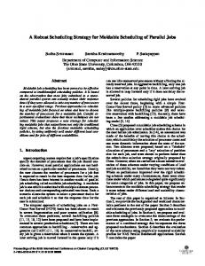
A simulation-based testing environment (see Figure 1) was created using SLAM II [3] to evaluate the performance of each of the scheduling approaches under various factory conditions. Each approach was coded in FORTRAN subroutines and the LRH and LRH-2 subroutines include calls to the CPLEX [4] optimization libraries to solve the network A group of N(30, 1.5) lots arrive to the drilling station every three (T) hours. The product type for each lot is randomly determined in accordance with each product’s relative probability of manufacture. This is determined by a product family’s probability of manufacture as well as the individual product’s probability of manufacture within the family. Each simulation run is for a month of operation, which is 160 releases to the drilling station. Repeat Each Order Release

Distribution of Lots Scheduling Policy

Simulator Generate Lots

Lots In Machine Status In

Optimization Model Determine schedule

Lots Assigned

Simulator Simulate system for one month

Evaluate: Makespan Number Late Total Overtime Average Finish Time Utilization

Figure 1: Simulation Testing Environment

5. Results And Discussion We developed two scenarios to assess the performance of five scheduling approaches. The two scenarios are: 1 Scenario with processing times variability factor v ranging from 0-1, but no equipment breakdowns. 2 Scenario with breakdown variability factor v ranging from 0-1, but deterministic processing times. The five scheduling approaches were evaluated to determine their performance for each of the five performance measures for both scenarios. Run times for scheduling a single lot release (30 jobs) averaged 0.2 seconds for the LRH method, 8 seconds for the LRH-2 method, and less than 0.01 seconds for ASDN, HASDN, and MFIFO. 5.1 Scenario #1 – No breakdowns, processing time variability The processing time variability factor included six values in the range of 0 to 1. The results for the performance criterion and scheduling methods are shown in Table 2 and the combined ranking in Figure 2. The makespan, average finishing time, numb er late and total overtime measures all have similar performance as the variability increases. At low variability levels, LRH-2 and LRH outperform the ASDN, HASDN, and MFIFO approaches. As the variability increases, ASDN performs better than LRH-2 and LRH. This is because this dispatching rule adapts to the variability present in the system by choosing a lot after some of the variability has been realized. Utilization is not impacted very much by the amount of variability in the system, as this is primarily determined by the specific jobs assigned to a particular machine. LRH-2 consistently has the best performance followed by LRH, HASDN, ASDN, and finally MFIFO. The combined ranking results for the five-performance measures (Figure 2) shows that the LRH-2 approach provides the best scheduling approach with respect to the manufacturer’s five performance measures when the process variability factor ν remains below about 60%. At that point, ASDN becomes the preferred approach. We note that even at v = 1.0, LRH-2 still significantly outperforms MFIFO. We conclude from this that except for cases with very high levels of processing time variability, that LRH-2 is the preferred approach. 5.2 Scenario #2 – Deterministic processing times, infrequent breakdowns with breakdown variability Scenario #2 has deterministic processing times, but includes equipment breakdowns. Machines randomly break down in accordance with a triangular distribution with a mean of 10 hours and require a repair time that follows a triangular distribution with a mean of 12 minutes. The variability factor ν ranged from 0 to 1 for the breakdown intervals and repair times. The results of the combined performance measures are shown in Figure 3. This scenario’s results are quite different from those of scenario #1. LRH-2 performs best for all levels of breakdown variability and LRH consistently performs next best. Thus, for a highly automated factory with little or no processing time variability but with equipment interruptions due to preventative maintenance or equipment jams, optimization routines can be very effective.

6. Conclusions In this research, we considered scheduling of the bottleneck operation of PWB manufacturing. Using a combined ranking of our five performance measures, we evaluated five approaches to scheduling this drilling area. The impact of processing time variability and equipment breakdowns were considered. In scenario #1, when there is processing time variability and there are no breakdowns, it was found that LRH-2 performed better than LRH throughout all the performance measures, and outperformed the other approaches with variability factor v between 0 and 0.6. Overall, the optimization approaches (LRH and LRH-2) outperformed the dispatching approaches (ASDN, HASDN, and MFIFO) when the processing time variability factor v is below 40%. In scenario #2, when there is breakdown variability and deterministic processing times, the optimization approaches outperformed the others across all performance measures. Figure 3 shows that the combined performance of LRH-2 was significantly better than that of LRH. We note that in all of our experimentation described in this paper, we limited the subgradient optimization procedure for LRH-2 to 70 iterations. Preliminary results have shown that even better performance can be obtained by increasing the number of allowable iterations. Obviously, more iterations means longer execution times, so an investigation into the number of iterations that balances the solution quality and solution time is warranted.

References 1. 2.

3. 4.

Yu, L., Shih, H.M., Pfund, M., Carlyle, W.M., and Fowler, J.W., "Scheduling of Unrelated Parallel Machines: An Application to PWB Manufacturing", IIE Transactions on Scheduling and Logistics, to appear. Pfund, M., Yu, L., Fowler, J., and Carlyle, W., "The Effects Of Processing Time Variability And Equipment Downtimes On Various Scheduling Approaches For A Printed Wiring Board Assembly Operation", Journal of Electronics Manufacturing, Vol. 11, No. 1, 2002, pp. 19-31. Pristker, A., Introduction to Simulation and Slam II, John Wiley & Sons, NY, 1995. CPLEX, Using the CPLEX Callable Library, Incline Village, NV, 1997.

Table 2: Scenario #1 Results Performance Measure

Variability 0 0.1 0.3 0.5 0.7 1 0 0.1 0.3 0.5 0.7 1 0 0.1 0.3 0.5 0.7 1 0 0.1 0.3 0.5 0.7 1 0 0.1 0.3 0.5 0.7 1

CMAX

Average Finishing Time

Utilization

Number Late

Total Overtime

LRH 4.93 4.96 5.16 5.57 6.23 7.61 2.78 2.79 2.83 2.92 3.05 3.33 79.4 79.4 79.4 79.4 79.3 79.1 5.07 5.09 5.24 5.61 6.23 7.45 4.85 4.92 5.5 6.73 8.88 14.1

LRH-2 4.87 4.9 5.09 5.43 5.93 6.97 2.74 2.75 2.79 2.86 2.97 3.21 78.4 78.5 78.5 78.5 78.5 78.4 3.89 4.25 4.8 5.28 5.87 7.13 4.16 4.25 4.8 5.87 7.54 11.4

ASDN 5.33 5.32 5.44 5.59 5.75 6.12 2.87 2.87 2.88 2.9 2.92 2.98 83.4 83.4 83.4 83.5 83.3 83.3 4.2 4.25 4.38 4.47 4.59 4.89 5.32 5.27 5.47 5.76 6.07 6.97

HASDN 5.71 5.62 5.93 6.23 6.71 7.99 2.86 2.85 2.88 2.92 2.98 3.13 82.9 82.9 82.9 82.9 82.8 82.5 3.99 4.02 4.17 4.3 4.48 4.76 5.31 5.17 5.61 6.21 7.14 9.42

1.20 1.00 0.80 0.60 0.40 0.20 0.00

LRH LRH-2 ASDN HASDN 0

0.2

0.4

0.6

0.8

1

MFIFO

Variability Factor v

Figure 2 Scenario #1 – Combined Performance Results

Scenario #2 Combined Ranking

Combined

Combined

Scenario #1(No Breakdowns) Combined Ranking

1.20 1.00 0.80 0.60 0.40 0.20 0.00

LRH LRH-2 ASDN HASDN MFIFO 0

0.2

0.4

0.6

0.8

1

Variability (Breakdown only)

Figure 3: Scenario #2 – Combined Performance Results

MFIFO 6.55 6.62 6.6 6.76 7 7.37 3.24 3.26 3.26 3.28 3.32 3.38 84.9 84.9 84.8 85 84.8 84.5 5.9 6.01 6.08 6.06 6.15 6.11 9.47 9.69 9.62 9.96 10.6 11.4