Development of an application using a clustering algorithm for ...

Development of an application using a clustering algorithm for definition of collective transportation routes and times Thiago C. Andrade1 , Marconi de A. Pereira2 , Elizabeth F. Wanner1 1

DECOM - Centro Federal de Educac¸a˜ o Tecnol´ogica de Minas Gerais - Campus II - Brasil 2

DTECH - Universidade Federal de S˜ao Jo˜ao del-Rei - Campus Alto Paraopeba - Brasil Abstract. This article presents the modeling, development and theoretical grounding for the development of an application based on the clustering algorithm DBSCAN, aiming to reduce the daily waste of time on the locomotion of a huge number of people to a common place. The clusters are created based on attributes, like the departure time of each person from its residence, the final destine and its both geographical locations (departure and arrival). People that compose the cluster are transported in a vehicle allocated according to the size of the cluster. A case study, with a specific group of people going to CEFET-MG Campus II, was conduct using a popular traffic simulator in order to measure the individual and the global time that people need to move, using the new transport arrangement. The simulation results were compared with a scenario where all people use public transportation. This comparison identified an average reduction of 45.80% in the time that people spent daily for their locomotion.

1. Introduction The traffic problems became more evident in the biggest metropolises in the last decades, due to the population growth. Thus, the Traffic Engineering started to have an important role in the traffic management of those cities, helping in the reduction of the problems arising from the huge number of vehicles on the streets, which contribute to the increase of locomotion time. Based on this scenario, the natural tendency is that each one tries to solve out their own locomotion problem independently, choosing the solution which demands less time, also providing comfort. However, finding the best solution for each single person is not feasible. Thus, the most promising way to make traffic conditions better is to identify groups with similar locomotion patterns (origin, destination and time) and propose a viable way for them travel together. Those groups of people are known in literature as traveling companions. Some relevant works were presented, e.g. [Tang et al. 2012], [Tang et al. 2013], introducing methods of grouping people. However the challenge continues, since most of the solutions proposed are not practical. The proposed problem can also be founded in literature related to school bus routing problem (SBRP) [Newton and Thomas 1969]. However, this class of problems considers many variables like bus garages and bus stop sequence, which increase the complexity of the problem [Park and Kim 2010]. On the other hand, it does not consider the possibility of using small vehicles, like cars, where a driver gives a ride to some neighbors. Using the concepts of clusterization, the latitude, longitude and locomotion time of the individuals can be collected and processed to group people that have similar loco-

motion time and also similar origin and destination. Then, it is possible to find routes that can transport these groups of people efficiently. Many works have been proposed, related to spatio-temporal clusterization, proposing improvements in the traffic, either through ride, new public transportation routes or even changing traffic orientation in streets and avenues [TORK 2012], [Kisilevich et al. ]. There is also the proposal of different clustering algorithms such as [Neill 2006], [Birant and Kut 2007] and [Rocha et al. 2010]. However, it was not found any work that proposes a broad arrangement methodology of transportation means (proposing combination of automobiles, vans and buses) directed to a group of people that share a common destination in a determined time of the day. More specifically, there is not any work that proposes a combination of transport arrangements with different capacities, for a group of students or workers that need to arrive at a specific destination (school or company) at a determined hour. Thus, this work presents as principal contribution the proposal of a methodology of spatio-temporal clusterization, aiming to find compositions and routes of means of transportation. This proposal is compared to the actual locomotion model, in which each individual locomotion is independent of the others, using the actual public transportation. According to [Tang et al. 2012], there are some aspects that are not adequately addressed by the works currently available in the literature. To name a few, it is possible to highlight: • Proximity in time and space: to move together, the objects not only need to be close in space, but also need to move in similar times. • Efficiency: the trajectories that are generated require, in fact, to reduce the locomotion times, also generating economy for the individual. • Effectivity: many people already have a locomotion route with a robust time and cost (e.g. people who live less than 700 meters of the working place) and hardly can have their cost and time reduced. In this case, the methodology has to keep its focus on the ones who demands more time to move. The proposed work aims to cover the questions presented by [Tang et al. 2012], and this will be detailed in the next sections. The paper is divided as follows. In section 2 it is detailed the used clusterization algorithm, besides the reasons why it was chosen as the base algorithm. Section 3 presents the modeling of grouping people problem, also as the application of an efficient solution for resolution. The section 4 contains a study-case developed, the parameters used and the results obtained. In section 5 there is a detailed analysis of the results and also a comparison with the actual scenario considered which everyone uses the public transportation. Finally, in section 6 the main conclusions of this work and the future works suggested are disposed.

2. Clusterization Algorithm - DBSCAN The first step of the problem modeling was the choice of a clusterization algorithm. Many procedures were tested, such as K-Means and variations and the DBSCAN. The K-Means algorithm and its variations were discarded after the tests with the database. These algorithms presented big variability of the results, being dependent on the choice of the centroid, and different values yield significantly different clusters. Moreover, these algorithms presented a strong tendency to generate only spherical clusters and there were

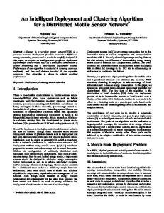
some difficulties in estimating the K parameter (number of clusters) for the algorithm execution. The choice of DBSCAN is justified after the satisfactory results obtained when it was applied on the studied database. Preliminary results showed the passengers were well distributed in the clusters and the number of noises was low. The details of the algorithm are presented below. The DBSCAN algorithm uses the local density of the points to determine the clusters. For a point X, a circle of radius  is defined around this point and, thus, we obtain his neighbors, as we can see in the Figure 1(a). For the existence of a cluster, it is necessary to have a minimum number of points inside this circle, i.e., it is necessary to have a minimum number of neighbors of the point X, defined by the parameter minPts. Thus, the algorithm iterates on the dataset, verifying dense regions and associating neighbors points to the same clusters, taking in count the condition of the minimum number of points by cluster (Figure 1(b)).

Figura 1. a) Point X and his neighborhood, by) Neighborhood expanded with the neighbor points of Y - Adaptation of [Zaki and Jr. 2013]

Since the algorithm considers the density of the points, not always the entire set of points will be associated to a cluster. There can be isolated points, in such a way that there are not a minimum number of neighbors to form a cluster. These points are considered as noises. Thereby, the algorithm consists of four steps: 1. All the point are initially associated to a cluster −1 and are marked as not visited. 2. Region Query Method: this method makes the search to find the neighbors of the actual point, called region query. The algorithm starts iterating over the points of the database and for each not visited point, the neighbors of this points are analyzed, according to the radius . If the number of neighbors of this point is higher than the minimum of points defined by the algorithm (parameter minPts), this point is associated to the actual cluster (the number of the cluster starts in −1 and is always incremented if this condition is satisfied) and all his neighbors are associated to the same cluster and marked as visited. If the number of neighbors of the points is lower than the parameter minPts defined, this point is considered as a noise and marked as visited. 3. Expand Cluster Method: for each point that was associated with a given cluster, the algorithm searches for neighbors of this point, which are inside a given radius , and associating them with the current cluster, marking them as visited. Thus, the current cluster is expanded. 4. The steps 2 and 3 are repeated until all point are visited and, thus, the final clusters are obtained and the noises too.

The main advantages of DSBCAN are: (1) The number of clusters do not have to be defined initially, differently from K-Means algorithm; (2) The algorithm is not so sensible to the incoming order of the points; (3) It can be defined the minimum number of elements per cluster; (4) There is the concept of Noise value, eliminating points of the database that are not relevant to the analysis. Amongst the main disadvantages, it is possible to highlight: (1) The algorithm is sensible to the choice of  parameter: if a big value is chosen we can have few clusters, and, choosing a low value, we can have many noises; (2) It is not so efficient when we have regions that are not so dense. The DBSCAN algorithm was modified and adapted to the problem. After the definition of each cluster elements, the following steps were done: (1) Calculation of the centroid of each cluster: the DBSCAN algorithm does not works with the centroid concepts. However, after the algorithm execution, the centroids were calculated as the mean of the points of each clusters, obtaining a central point with the mean latitude and longitude of each point of the cluster; (2) Optimization and allocation of the points: with the definition of the centroid concept, some points can change from one cluster to another, since they are near to a new defined centroid. Thus, for each point, it was verified its distance in relation to the centroid, guaranteeing that they was associated to the nearest centroid. The pseudocode for those changes, can be seen in Algorithm 1 and Algorithm 2: Data: Points, Latitude and Longitude Result: Cluster, Centroids for i ← 0 to i ← N umberOf Clusters do for j ← 1 to j ← N umberOf ClusterP oints do ClusterLatitude(i) += PointLatitude(j); ClusterLongitude(i)+=PointLongitude(j); numberOfElements++; end ClusterLatitude(i) = ClusterLatitude(i) / numberOfElements; ClusterLongitude(i) = ClusterLongitude(i) / numberOfElements; numberOfElements = 0; end Algorithm 1: Step 1 - Calculate the cluster centroids Data: Points, Latitude and Longitude Result: Points, Allocation for i ← 1 to i ← N umberof P oints do for j ← 0 to j ← N umberOf Clusters do if HaversineDistance(i,CentroidOfCluster(j)) ≤ HaversineDistance(i,CentroidOfOriginalCluster) then Move point i, to Cluster j; end end end Algorithm 2: Step 2: Optimization and allocation of the points

3. Problem Modeling In order to limit the problem scope and to find a solution that improves the daily locomotion time of people, the problem was divided into two parts. In the first part of the problem, people were divided into clusters, according to the algorithm DBSCAN. For each cluster (Ci ), a centroid was calculated (Ki ) and was defined as departure point for people in that determined cluster. Thus, in the first part of the locomotion route, each people (Xi ) walk to this central point, spending one initial walking time (T ci ). It was defined that the walking time can be no more than 20 minutes. The distance of each individual (Xi ) to the centroid was calculated using the Haversine Function and the the locomotion time estimate until the centroid (T ci ) was defined as the average walking time of 3 miles/hour per person. For example, considering the distance of a determined person to the centroid of its cluster of 0.5 miles, the person would walk for about 10 minutes until reaching the centroid. In the second part of the problem, after all people walked to the centroid of its respective cluster, the route would be done from one or more vehicles. The type of the vehicle(s) was chosen according to the number of people allocated in each cluster, as below: • • • •

Up to 5 persons - car; 6 to 15 persons - van; 16 to 40 persons - bus; More than 40 persons - combination of vehicles, according to the number of persons.

Thus, after the choice of the most adequate vehicle, the rest of the route would be done without stops until the final destination. The locomotion time from each cluster to the destination is given by (TK j). The locomotion time of each vehicle until the final destination was calculated using Google Maps data, obtaining the time directly from the route selected by Google algorithm. Finally, the obtained time was compared to the actual time spent by using public transportation (% of saved time). For an estimate of the actual time spend for each person, it was used the Google Maps data, considering the public transportation (bus and/or subway). The problem can be modelled as follow: min totalLocomotionT ime =

n X i=1

subject to: T ci ≤ 20 minutes, Ti ≤ T ai in which Ti = T ci + T kj ,

Ti

(1)

n = number of persons, Ti = total locomotion time of person i, T ci = walking time of person i, T kj = locomotion time from the centroid j to the destination. T ai = actual locomotion time of person i.

Figura 2. Proposed problem modeling, with 10 persons and 2 clusters.

Figure 2 illustrates the proposed model, considering a group of 10 persons and 2 clusters. It is possible to observe that which people were associated to each cluster, the centroid of each cluster and the type of vehicle chosen. For the application execution it is necessary to inform the  e minPts parameters of DBSCAN algorithm, as well as the desired arrival time at the destination for all points. The results can be summarized into two isolated screens. The first one (Figure 3) presents the summary of the data obtained in a grid, for each cluster, containing the following information: • For each cluster: cluster number, latitude and longitude of the centroid, number of elements, distance to the destination in meters and minutes. • For each cluster point: point ID, latitude and longitude, distance to the centroid in meters, walking time in minutes to the centroid (also informing the departure time for each point, according to the total spending time and including a margin of 10 minutes to eventual delays), total time spent, bus time, time saved in minutes (also informing the % of time saved).

Figura 3. Grid with the data obtained, example of cluster 0 and visualization of two points

Figura 4. Visualization of the cluster obtained and its points on the Map, example of cluster 7, with 10 points (some of them very close to each other)

Figure 4 shows how the data was presented on Google Maps, divided by clusters. According to Figure 5, the first step for the clusterization is the selection or extraction of characteristics to be studied. For our problem three characteristics were chosen: latitude, longitude and arrival time at CEFET-MG Campus II.

Figura 5. Clusterization Procedure - [Xu and Wunsch 2005]

For tests and validation, a database containing the localization (latitude and longitude) of 437 persons was used. In order to obtain relevant information to the problem and the validation of the final results obtained, the Directions API of Google Maps was used. Particularly, the API was used to establish the routes and the time required to run them, using car (or van), bus or walking, when necessary.

4. Experiment and Results For the execution of the experiment, the following values were chosen for DBCSAN algorithm:  = 1500 meters and minPts = 5. The destination chosen was the Centro Federal de Educac¸a˜ o Tecnol´ogica de Minas Gerais Campus II - CEFET-MG in Belo Horizonte (latitude = -19.9377, longitude = -43.9997) and the arrival time at destination was defined as 7 AM. The value of  was chosen according to the problem modeling. Since T ci ≤ 20 minutes, using  = 1500 meters, the locomotion time of the neighbors to the central point is 18 minutes at most, according to the walking time defined. The value of minPts was chosen based on the maximum number of passengers that can be transported in a car (the mean of transportation with the minimum of passengers) and to optimize the transportation, aiming always to transport the maximum number of people per vehicle.

The experiment generated 33 clusters, transporting an total of 394 persons, which represent about 90.2 % of the total. The other 43 persons were treated as noises, since they were in low density regions, not covered by the algorithm. The points were distributed according to the density of each region, covering all the means of transportation available. There were generated clusters varying from 5 up to 70 passengers. According to the  parameter defined, the biggest walking locomotion time was 23.04 minutes, from point 184 to the center of cluster 5. This value is acceptable, since it is only 3 minutes higher than the previous value defined (15% variation). In Figure 6 it is shown the clusters generated and how they were distributed on the map. The figure shows the distribution of the clusters generated in the city of Belo Horizonte and the mean of transportation defined for each cluster.

Figura 6. Clusters obtained in the application

Table 1 summarizes the clusters found, showing the number of elements obtained on each one and the average time saved by each cluster. It is important to highlight that, to compute the average saved time, it was considered the walking time necessary to each person leave its home and arrives in the stop point. In the first case, using the conventional public transportation, people walk from their home to the bus stop; in the second case, using the proposed approach, people walk from their home to the bus/van/car stop point (centroid of the cluster). In both cases, the Google Maps API was used to determine the walking time of each person.

5. Analysis of Results Through the analysis of results, we can verify that the cluster which biggest saved time is was the cluster 32, with an average of more than 1 hour and 10 minutes saved per person. The worst result, and the only cluster where there was not saved time, was the 15, with an average delay of 2 minutes and 40 seconds per person.

Tabela 1. Results obtained with DBSCAN algorithm,  = 1500 meters and minPts =5 Cluster

Number of Elements

Average Time Saved

0 1 2 3 4 5 6 7 8 9 10 11 12 13 14 15 16 17 18 19 20 21 22 23 24 25 26 27 28 29 30 31 32 Total Noises

14 25 9 8 11 70 38 10 7 7 9 20 6 23 16 7 5 5 10 6 5 6 5 5 5 6 11 5 10 5 7 10 8 394 43

45.57 49.58 33.58 39.48 22.35 16.43 23.56 9.53 54.73 56.11 43.31 37.77 19.51 64.41 23.67 -2,69 2.62 56.21 24.80 25.29 37.96 54.48 53.59 28.89 25.84 26.65 21.00 53.88 67.71 55.85 33.29 67.51 70.30 34.51

Analyzing Table 2, we can verify how the points were distributed on the cluster 32. In Figure 7 it is highlighted the cluster 32 with its points (in the top) and the localization of CEFET-MG (in the bottom), being possible to verify the distance between them. Table 3 shows the data from cluster 15. The points of cluster 15 are shown on the map in Figure 8. Tabela 2. Points distributed on the cluster 32 Point

Centroid Distance

Walking Time

Total Time

Bus

Saved Time (% saved)

221 230 329 330 331 332 338 344

662.68m 662.64m 779.54m 590.08m 376.96m 821.30m 789.05m 532.90m

7.95min 7.95min 9.35min 7.08min 4.52min 9.86min 9.47min 6.39min

38.40min 38.40min 39.80min 37.53min 34.97min 40.31min 39.92min 36.84min

108min 108min 99min 105min 119min 106min 114min 109min

69.97min (64.56%) 69.97min (64.56%) 58.80min (59.63%) 67.52min (64.27%) 84.08min (70.62%) 65.42min (61.88%) 74.20min (65.02%) 72.46min (66.29%)

Verifying the location of the clusters on the map, we can see that the result obtained on the cluster 15 is justifiable, since all points of these clusters are really close to CEFET-MG. For this dataset, the proposed solution would not be adequate, since for those people is better to walk directly to CEFET-MG than walking to the centroid and

Figura 7. Visualization of cluster 32, its points and the distance in relation to CEET-MG Tabela 3. Points distributed on the cluster 15 Point

Centroid Distance

Walking Time

Total Time

Bus

Saved Time (% Saved)

30 32 65 80 81 154 177

368.90m 489.54m 364.30m 505.91m 507.18m 1,125.60m 372.29m

4.43min 5.87min 4.37min 6.07min 6.09min 13.51min 4.47min

13.81min 15.26min 13.75min 15.45min 15.47min 22.89min 13.85min

10min 32min 10min 3min 1min 33min 4min

-4.13min (-42.67%) 16.51min (51.97%) -3.82min (-38.52%) -12.52min (-427.45%) -14.69min (-1883.27%) 9.74min (29.85%) -9.93min (-253.34%)

Figura 8. Visualization of cluster 15, its points and the distance in relation to CEET-MG

then get the public transportation. On the other hand, for the cluster 32, localized far away from CEFET-MG, we can check the efficacy of the proposed solution. The average time saved for this cluster is really high and, in the worst case, the saved time is 58.80 minutes, which represents an economy of 59.63% of the previous time spent by this person using public transportation. In the Figure 9, we can see how the saved timed is strongly related to the distance of the points and CEFET-MG. For the points highlighted in green, we obtained the highest saved times: 70.30 minutes for the cluster 32, 67.71 minutes for the 28, 67.51 minutes for the 31, 64.41 minutes for the 13 and 56.21 minutes for the 17. For the points in the red region, we obtained the worst saved times: -2.69 minutes for the cluster 15, 2.62 minutes for the 16 and 9.53 minutes for the 7. In this way, we can conclude that the factor which has the most influence on the saved time for a point is its distance to the destination. For points relatively far from the destination, the efficiency of the algorithm is really high, with an average save time

Figura 9. Visualization of the clusters with higher saved time (green) and smaller saved time (red).

closer to 65%. On the other hand, for points closer to the destination, the efficiency of the algorithm is lower, and can be negative in points really closer to the destination. For intermediate points, the average saved time is really satisfactory, with an average of 34.51 minutes saved per person, which represent an economy rate of 45.80% in the average. Finally, some points are marked as noises as can be seen in Figure 10. We can verify that those points are more isolated, being unable to associate them to a cluster. In some case, despite of having close points, they do not meet the requirement of the parameter minPts to form a new cluster.

Figura 10. Some points marked as noises

6. Conclusion and Future Works According to the obtained results, we can conclude that the problem modelling and the application developed have reached the proposed objectives on the work. The result obtained has a highly relevance, since it not only can helps the reduction of people daily

locomotion time, but also contributes to the reduction of traffic in the cities, encouraging means of public transportation or carpooling directed to the needs of their users. The application can be used in transportation of large masses of people to a specific location. Certainly, an average economy of 45.80% of locomotion time is something really relevant, which shows that simple solutions well-modeled can help to reduce one of the metropolises big problems, that is the traffic and loss of time in locomotion. Thus, the main contributions of this paper are: (1) An efficient application to reduce the daily locomotion time of a large number of persons until a common destination; (2) To incentive collective transportation (bus, vanpooling and carpooling), reducing the number of vehicles on the streets and contributing for a better traffic; (3) Adaptation of a clustering algorithm and modeling of an application to solve traffic problems. As a continuity of this work, the following issues are proposed: (1) Algorithm improvements to work with Google distance function, obtaining traffic data during the displacement; (2) Pre-processing of the data using the UTM (Universal Transverse Mercator) coordinates system in order to simplify the distance calculation; (3) Insertion of time factor on the algorithm, working with people locomotion in different hours.

Referˆencias Birant, D. and Kut, A. (2007). St-dbscan: An algorithm for clustering spatial temporal data. Data and Knowledge Engineering, 60(1):208 – 221. Kisilevich, S., Mansmann, F., Nanni, M., and Rinzivillo, S. Spatio-temporal clustering: a survey. Neill, D. B. (2006). Detection of spatial and spatio-temporal cluster. School of Computer Science, Carnegie Mellon University. Newton, R. M. and Thomas, W. H. (1969). Design of school bus routes by computer. Socio-Economic Planning Sciences, 3(1):75 – 85. Park, J. and Kim, B.-I. (2010). The school bus routing problem: A review. European Journal of Operational Research, 202(2):311–319. cited By (since 1996)38. Rocha, J., Oliveira, G., Alvares, L., Bogorny, V., and Times, V. (2010). Db-smot: A direction-based spatio-temporal clustering method. In Intelligent Systems (IS), 2010 5th IEEE International Conference, pages 114–119. Tang, L.-A., Zheng, Y., Yuan, J., Han, J., Leung, A., Hung, C.-C., and Peng, W.-C. (2012). On discovery of traveling companions from streaming trajectories. pages 186–197. Tang, L.-A., Zheng, Y., Yuan, J., Han, J., Leung, A., Peng, W.-C., and Porta, T.-L. (2013). A framework of traveling companion discovery on trajectory data streams. ACM Transactions on Intelligent Systems and Technology, 5(1). TORK, H. F. (2012). Spatio-temporal clustering methods classification. DSIE - Doctoral Symposium in Informatics Engineering. Xu, R. and Wunsch, D. C. (2005). Survey of clustering algorithms. IEEE Transactions on Neural Networks, 16(3):645–678. Zaki, M. J. and Jr., W. M. (2013). Data Mining and Analysis: Fundamental Concepts and Algorithms.