Development of an Artificial Neural Network to Predict ... - J-Stage

ISIJ International, Advance ISIJ Publication International, by Advance J-STAGE,Publication DOI: 10.2355/isijinternational.ISIJINT-2016-368 by J-STAGE ISIJ International, J-Stage Advanced ISIJ International, Publication, ISIJ International, DOI: Advance http://dx.doi.org/10.2355/isijinternational.ISIJINT-2015-@@@ Vol.Publication 57 (2017), No. ISIJ by J-Stage 1International, Vol. 57 (2017), No. 1, pp. 1–9

Development of an Artificial Neural Network to Predict Sulphide Capacities of CaO–SiO2–Al2O3–MgO Slag System Alvin MA,1) Sina MOSTAGHEL2) and Kinnor CHATTOPADHYAY1)* 1) Department of Materials Science and Engineering, University of Toronto, Toronto, M5S 3E3 Canada. 2) Technology Development Group, HATCH Ltd, 2800 Speakman Drive, Mississauga, ON, L5K 2R7 Canada. (Received on June 18, 2016; accepted on September 21, 2016; J-STAGE Advance published date: November 30, 2016)

Depletion of the high quality ores around the world has forced ferronickel producers to extract metal values from low-grade ore bodies with significant amounts of impurities. Under this condition, maintaining alloy quality is of utmost importance for the smelters; however still, accessibility of a reliable sulphide capacity model for FeNi refining processes is an issue. Many of the current models, such as those incorporating optical basicity, have proven to be erroneous and unreliable for wide ranges of composition and temperature. These models are typically developed and tested without a proper validation method thus allowing for great correlations which may not fare well with the introduction of new data. Models built from fundamental thermodynamic data perform much better in predicting sulphide capacities but are not only complicated to formulate but also too complicated to be used by operators on a day to day basis as multitude of inputs are needed. Hence, development of a reliable model based on fundamentals, which can also be directly used by plant operators is very much demanded by the industry. In the current study, an artificial neural network (ANN) approach has been used to predict sulphide capacities of slag compositions in the CaO–SiO2–Al2O3–MgO system with an objective to be used in ferronickel refining processes. The resulting models are evaluated on: 1) coefficient of multiple determination (R2), 2) correlation strength (r), 3) root mean square error (RMSE) and 4) computation speed. The ANN based model has shown to be superior in predicting sulphide capacities to current models. KEY WORDS: ferronickel refining; artificial neural network; FactSage; optical basicity.

the machine learning technology into chemical process metallurgy. Thus an ANN approach was employed by the authors to explore its potential application in process metallurgy with specific emphasis on desulphurization.

1. Introduction The refining of crude metal is of utmost importance due to stringent quality demands and a deterioration in ore quality. In particular, sulphide capacities which is a measure of the sulphide removing power of the slag, is an important metric which should be optimized in order to obtain a desired final product. Despite the wealth of knowledge in the modeling domain, most of the models have largely become stale. The work presented here will tackle sulphide capacity modeling from a new perspective. Artificial neural network (ANN) modeling has been used in many different fields. This type of predictive statistics has thrived in the present surge in computing power and as a result, has risen to the forefront of many different industries. Some of its applications include investment forecasting,1) speech recognition,2) and control systems.3) Its perforation into the metallurgical field has largely been non-existent. Only a few researchers in metallurgy have employed machine learning algorithms much less neural network based ones.4–8) The research presented here attempts to cross-pollinate

2. Sulphide Capacity Sulphur in the slag can be described by the following equilibria: Gas-Slag Metal-Slag

1 S2( g ) + (O2 − )slag = S2 − 2

( )

slag

1 + O2( g ) ..... (1) 2

[S]metal + (O2 − )slag = ( S2 − )slag + [O]metal ... (2)

Equation (1) describes the equilibrium between the slag and gas phase in terms of relative partial pressures of both sulphur and oxygen. Comparatively, the sulphur system can also be approached from the metal-slag equilibrium (Eq. (2)). Both systems reveal two components imperative for efficient desulphurization: 1) O2 − and thus basicity must be sufficiently high and 2) the [O] content must be low. Many fluxing reagents are typically employed to meet these prerequisites. To quantify the desulphurization of a melt, Fincham et al.9) introduced the concept of sulphide capacity. Since its conception, the sulphide capacity has been the focus of

* Corresponding author: E-mail: [email protected] DOI: http://dx.doi.org/10.2355/isijinternational.ISIJINT-2016-368

1

© 2017 ISIJ

ISIJ International, Advance Publication by J-STAGE ISIJ International, ISIJ International, Advance Vol.Publication 57 (2017), No. by J-Stage 1

Similarly, Taniguchi et al.,13) defined the relationship presented in Eq. (7) to account for sulphide capacities in the CaO–Al2O3–SiO2–MgO–MnO system. In this system low SiO2 were investigated. While good adherence is seen with experimental work, validation of the regression was not apparent.

various modeling attempts to understand desulphurization from a chemical standpoint. Fincham et al.’s relationship can be derived from the equilibrium coefficient (Eq. (3)) of the gas-slag reaction as seen in Eq. (1). Fincham et al.’s definition of sulphide capacity can then be derived through manipulation (Eq. (4)). The correlation also reveals the need for atmospheric and temperature control for efficient sulphur removal.

Ke (T) =

1 2 O2

P × fS × ( %S)slag 2−

1 2 S2

LogCs = 7.350 + 94.89logΛ −

T +0.2284 ( wt − %SiO2 ) + 0.1379( wt − %Al 2 O3 )

.................... (3)

P × a O2−

CSs/g =

K e × a O2− = ( %S)slag fS2−

+0.0841( wt − %MnO )

PO2 ................ (4) PS2

22 690 − 54 640 Λ + 43.6 Λ − 25.2 ......... (5) T

E + A .............................. (8) T

15 864   15 893 − 4.49  Λ  ........ (9) LogCs = −6.08 + + Λ T

3.2. Short Range Order Similarly, sulphide capacity modeled from short range order comes with a host of its own problems. Some of the more famous frameworks in this area have been incorporated into proprietary software such as FactSage (developed by CRCT and GTT Technologies),16,17) and ThermoSlag (developed by the Royal Institute of Technology (KTH)).18) Comprising many different databases as well as frameworks, FactSage is an all-purpose thermodynamics software. It’s sulphide capacity framework, developed by Kang and Pelton,16) is based on the extrapolation of all permutations of cations and anions on a pseudo-lattice. The resulting model has shown great correlation to experimental results in a wide range of slag systems.16) The advantages of FactSage are clear, however the formulation of a model such as this requires many building blocks such as an already established method for handling and accounting for randomness.19) Much like the formulation, the use of FactSage is equally complicated. Furthermore, inherent to its formula-

LogCs = −13.913 + 42.84 Λ − 23.82 Λ2  11 710  −  − 0.02223 × wt − %SiO2 − 0.02275…  T  ×wt − %Al 2 O3 Λ ≥ 0.8 LogCs = −0.6261 + 0.4808Λ + 0.7197Λ2  1 697   2 587Λ  + −  + 0.0005144 …  T   T  ×wt − %Al 2 O3

© 2017 ISIJ

LogCs =

While exhaustive, these models do not capture the system in its entirety (covering the entire temperature and compositional ranges pertinent to FeNi refining). Furthermore, a common downfall to these models has been the method in which they have been formulated. The model development is extensive; however, the model validation often employs a non-split data set and thus may not suffice as a thorough assessment of the correlation.

In Young et al.’s model12) a new regression term, Λ2, was introduced and the correlation discretized. Based solely on the assumption that a non-linear relationship dominated the optical basicity relationship, Young et al. formulated a new relationship shown in Eq. (6). This model better described sulphide capacity than the previous Sommerville et al. model11) but could not effectively handle slags with high FeO due to an underestimation of its molecular optical basicity.14,15) Λ < 0.8

........................................... (7)

In the most recent iteration of the optical basicity based modeling approach, Zhang et al.14) proposed a correction to the molecular optical basicity of FeO, increasing it from 1 to 1.24. Also included in Zhang et al.’s model is the inherent assumption that a linear relationship exists between the reciprocal of optical basicity and the pre-exponential factor, A (Eq. (7)). The relationship is shown in Eq. (8). While sufficient for most slag systems, Zhang et al.’s model14) has shown fundamental mismatch at high sulphide capacities for slag compositions in the CaO–SiO2–Al2O3–MgO system.14)

3.1. Empirical Modeling Sulphide capacity has been modeled through both empirical relationships and through modeling of short range interactions: Empirically, the most common and extensive models are those developed using optical basicity. First proposed by Duffy and Ingram,10) optical basicity uses the ratio between the electron donor power of oxides in glass and electron donor power of oxide ions to predict sulphide capacity. This paved the way for significant models by Sommerville et al.,11) Young et al.,12) Taniguchi et al.13) and most recently Zhang et al.14) Sommerville et al.’s11) model uses a combined regression correlation to describe sulphide capacities. The model uses a temperature (1 573 K–1 973 K) correlation at various iso-optical basicities to model sulphide capacity. The unifying expression is shown in Eq. (5). While versatile, Sommerville et al.’s relationship was found to be inaccurate at higher sulphide capacities.12) LogCs =

…

−0.0587( wt − %MgO )…

3. Sulphide Capacity Modeling

10 051 + Λ ( −338( wt − %MgO ) + 287( wt − %MnO ))

........................................... (6) 2


tion, the inputs into FactSage are set and are invariable. In the KTH model, a specially defined interaction coefficient (ξ) was proposed to model high FeO slags. This new metric is defined in Eq. (10) and an integral part in its prediction mechanism. A major advantage of this model is its ability to predict slags of lower order therefore, an application to ferronickel refining slags plausible. However, similar to FactSage, the formulation of the interaction parameters requires advanced experimental work. Given the associated costs and difficulties with experiments, some interaction parameters may not be measurable or estimated accurately. An excerpt of the formulation applicable for ferronickel refining is shown in Eq. (11).

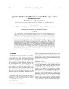
Although these fundamental models are much more accurate than their empirical counterparts, these models frequently require advance fundamental knowledge which are at times derived from experimental work. These myriad of inputs constitute a model unattractive for general use in pyrometallurgical plants. 4. Artificial Neural Network Development 4.1. Visualization Data on sulphide capacities of the CaO–SiO2–Al2O3–MgO system have been gathered from 15 different studies.9,13,20–32) These studies examine different aspects of the slag system and thus represent a good staging point for the modeling of the whole spectrum of sulphide capacities. The variables of interest were those that are chemically pertinent to the determination of sulphide capacity (LogCs). These are: 1) wt-% CaO, 2) wt-% SiO2, 3) wt-% MgO, 4) wt-% Al2O3, 5) wt-% (S)slag, 6) ( Po2 / Ps2 ) , and 7) temperature. Further, as recommended by Fincham et al.,9) only the studies using an equilibrium time higher than 4.5 hours were considered. The entire data set used in this work is illustrated in a scatter plot shown in Fig. 1. Figure 1, has been laid out in such a way to promote insight gathering. The relative correlation strengths are shown in Fig. 1 in different shades of colour. Red (high),

a o2 −  ξ  ......................... (10) = exp  −  fs2−  RT 

RT(loge Cs ) = 58.8157 × T − 118 535… − ( X Al2 O3 ×157 705.28 − X CaO × 33099.43 + X SiO2 ×168872.59 + X MgO × 9 573.07)…

(

Al2 O3 −CaO Al2 O3 −CaO−MgO CaO−SiO2 MgO−SiO2 2 O3 −SiO2 − ξ interaction + ξ iAl + ξ interaction + ξ interaction + ξ interaction … nteraction Al2 O3 −MgO−SiO2 CaO−MgO−SiO2 Al2 O3 −CaO−SiO2 +ξ interaction + ξ interaction + ξ interaction

)

......................................... (11)

Fig. 1. Scatterplot of CaO–SiO2–Al2O3–MgO system, compiled from9,13,20–32) and ordered by relative correlation strength. Red, blue and beige represent high, medium and low correlation. (Online version in color.)

3

© 2017 ISIJ


blue (medium), and beige (low), are used as the basis of ordering in the figure. The correlation strength quantifies the strength of a linear relationship between two variables. When the correlation is weak there is no tendency for the variables to linearly move with respect to each other. Correlation can be calculated between the variances of two variables and its covariance. These are shown in Eqs. (12) and (13) respectively. The correlation can then be defined in Eq. (14).

∑ (i − ī ) Var ( i ) =

n i = x, y

Covar ( x, y ) =

r=

(columns as variables, rows as unique data points) and Wi,k as a matrix which represents the synapse weights, the relationship at the hidden layer for n data points in the set (training or testing), i variables (Table 1) and k number of hidden nodes can then be described as:   X1,1 X1,i   W (1) W (1)   1, k    1,1 1 f ( )    ×    = A ...... (15)     X n,1 X n,i   Wi(,11) Wi(,1k)     

2

.......................... (12)

Where f is an activation function and, A is the resulting matrix which will be passed on to the synapses posthidden nodes. Similarly, the outputs of the hidden nodes are weighted and then transformed a final time before a prediction can be formed:

∑ ( x − x ) × ( y − y ) .............. (13) n

Covar ( x, y ) Var ( x ) × Var ( y )

  A1,1 A1, k   W ( 2 )   1    ˆ 2 .......... (16) f ( )    ×    = Y   A    2 n ,1 A n , k    Wk( )   

...................... (14)

The ordering of Fig. 1 is expected based on the chemical relationship (Eqs. (1) and (2)) derived from the initial sulphide capacity work by Fincham et al.9) shown in Eqs. (3) and (4). Strong correlation is seen with wt-% CaO, wt-% SiO2, wt-% Al2O3 and wt-% (S) slag. One small caveat of the analysis shown in Fig. 1 is that the ordering is relative. Thus factors such as the root of the pressure ratio and temperature may not appear to be highly correlated but in reality are important factors to consider in the scope of absolute correlation.

Optimization occurs after each prediction, thus the weights are constantly changing. The method in which weights are corrected will vary depending on the learning algorithm used. To exploit the convex nature of quadratic equations, sum of squared errors is commonly used as a cost function to optimize the weights. This is defined as Eq. (17):

J=

(

( (

)

1 1 2 2 1 ∑ Y − f ( ) f ( ) X n,i Wi(,k) Wk( ) 2

)) ........ (17) 2

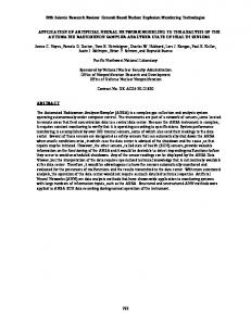
Brute forcing this equation is near impossible for high dimensional problems thus a gradient descent algorithm is utilized to solve the optimized path. Akin to dropping a ball and letting it roll towards the path of least resistance, the gradient descent algorithm solves the cost function by finding the path of lowest slope. The direction of the ball is determined iteratively with each step coming from each data point from the training set. This method shortens the time needed to identify a minimum. Once a minimum is found, the weights can then be used as a basis for a predictive model. At this point the testing portion of the dataset can be used. The entire process is depicted in Fig. 3.

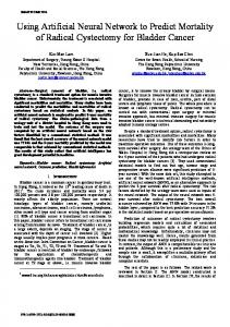
4.2. ANN Fundamentals Instead of a singular equation, an ANN uses numerous equations which account for the relationships between nodes, synapse weights, output and inputs (Fig. 2). This complex interplay of relationships can be described through matrices. Defining Xn,i as a matrix representing the inputs

Table 1. Different ANN models that were considered for the current investigation. Model Model Model Model Model Model Model 1 2 3 4 5 6 7 Hidden Nodes

5

5

Wt-% MgO

Fig. 2. Basic ANN architecture with a single hidden layer. Where (—) are synapses. (Online version in color.)

© 2017 ISIJ

4

5

3

7

X

3

7

X

X

Wt-% CaO

X

X

X

X

X

X

X

Wt-% SiO2

X

X

X

X

X

X

X

Wt-% Al2O3

X

X

X

X

X

X

X

Wt-% (%S)slag

X

X

X

X

X

X

X

PO2 PS 2

X

X

X

X

X

X

T

X

X

X

X

X

X


Fig. 3. Flowchart for an artificial neural network model. (Online version in color.)

will be considered in the current work. The number of nodes forming the single layer will vary according to Table 1. To introduce non-linearity into the system, a sigmoidal activation function, the logistic function, will be used (Eq. (18)). W will change depending on the location of calculation (Wi,k for synapse weights prior to the hidden node and Wk for synapse weights after the hidden node).

f ( X n,i W ) =

1

..................... (18) 1+ e ˆ ) is the sulphide With reference to Fig. 3, the output ( Y capacity of each data point while the inputs (I) will vary in accordance with Table 1. Similar to any regression method, the inputs will consist of easily accessible metallurgical inputs such as dissolved sulphur in slag or chemical composition.

Fig. 4. Errors associated with gradient descent use. Adapted from reference 34.34) (Online version in color.)

Although faster, the gradient descent algorithm has major drawbacks. Unless the cost function has been solved in all domain and range (at sufficient resolution), errors may be masked by the results. These possible errors are 1) detection of a faulty minima 2) quasi-stand still and 3) the departure from a suitable solution (Fig. 4). Any of these errors will lead to improper training of the ANN and thus a faulty model. To avoid errors such as these, the step size or learning rate must be carefully defined.

− ( X n ,i × W )

4.4. Model Validation Approach The simplest form of cross validation, the hold out method, is used to validate the ANN models. In this method, a certain percentage of the dataset is sampled to train the algorithm (training dataset) while the remaining data (testing dataset) is used to validate the model. To avoid overtraining and because the dataset is sufficiently large, the split ratio between testing and validating data sets will be 50:50. As samples are taken randomly, careful measures were enacted to ensure sampling quality. As prescribed by past work in the evaluation of different ANN models,37) the principal framework that will be used to compare different models studied here, are: 1) Coefficient of multiple determination (R2): is a measure of goodness of fit between predicted and actual values. This can be found through the squaring of the correlation coefficient 2) Correlation coefficient (r): is derived in Eqs. (1) to (3) and is a measure of linear strength between predicted and actual values 3) Root mean square of errors (RMSE): is the absolute average distance between predicted and actual value and is defined as:

4.3. Model Formulation Currently there are many software products available both commercially and open source, which can provide basic prediction architecture. Because of its accessibility, the open source R programming language,33) known hereafter as R, is employed as the basis of the modeling approach. The modeling approach in the current work utilizes a sigmoidal-regression artificial neural network model using a globally resilient backpropagation algorithm developed by Anastasiadis et al.34) Other learning algorithms such as the traditional back propagation algorithm, which uses a set learning rate have proven unreliable due to many factors.35,36) Its most frequent issue is that it is extremely time-consuming and often results in a partial training of the dataset due to a local minimum convergence of the error function. Aiding this issue requires advanced knowledge of the optimal hidden nodes, starting weights and optimal learning rate. However; these metrics are rarely available thus using a backpropagation algorithm is unattractive. The method developed by Anastasiadis34) uses an adaptive learning rate which aids in better convergence speed and stability. The theorem and corresponding proof of this method can be found in reference 34.34) Only one hidden layer (between output and input layers)

RMSE =

∑ ( Y − Yˆ )

2

..................... (19)

n

Often overlooked or outright ignored, the computation time is an important factor to consider, when qualifying an algorithm for industrial scale use. Although computation time for a dataset of the current size is irrelevant within a 5

© 2017 ISIJ


small dataset, in industry the requirements are much different. The computational speed will increase significantly with increasing sensors, compositions, temperatures and sampling intervals. In the work presented here, time will be defined as the time it takes for the optimization of matrix W and will be the final criterion used to evaluate different ANN models presented here.

7, may also result in better predictions; however, was not investigated further due to the possibility of overfitting the data. Furthermore, MgO seems to have a relatively more pronounced effect for 3 and 7 node networks. The RMSE has shown a slight decrease with MgO present as a predictor. This suggests one of two things: 1) convergence of the cost function to a local minima or 2) global translation of the cost function upwards. The resemblance of the models with and without MgO suggests that any convergence or vertical translation may be only minimal. Because of this, a network which does not deploy MgO is preferred. The predicted LogCs values have been compared with the actual LogCs (testing dataset) values from Figs. 5–11. Also included is the ideal predictor line. This line, described by a slope of 1 and an intercept of (0,0), shows a model’s fidelity to an ideal model (Actual LogCs = Predicted LogCs). By inspection, Models 2, 3, 5, and 7 are much closer to ideal than the rest. Therefore, on the basis of the current dataset and validation approach, any of these architectures are applicable.

5. Results and Discussion 5.1. ANN Models The ANN models developed in accordance with Table 1, was benchmarked under the 4 previously criteria. They have been trained using the training dataset and validated using the testing dataset. The adequacy of each model has been presented in Table 2. Based on only the highly correlated variables shown in Fig. 1, model 1 performed the worst. Without including ( Po2 / Ps2 ) , and temperature, an artificial neural network trained using the remaining variables was unable to accurately predict changes in the sulphide capacity. This was also evident in Fincham et al.’s original sulphide capacity relationship.9) Models 3 and 4 tested the need of MgO. The correlation between MgO and sulphide capacity is a highly contested matter. From literature, the deployment of MgO was found to be highly model dependant. In Taniguchi et al.’s model,13) MgO was positively correlated with sulphide capacity. Similarly, work by Kang et al.16) using FactSage predicted a positive correlation but only at high mole fractions ( > 0.6). Conversely, KTH’s Thermoslag,18) showed a negative correlation.13) Both models by Sommerville et al.11) and Young et al.12) showed negligible effect of MgO. In the work presented here, MgO was shown to be trivial in the prediction. However, it is important to note that the maximum MgO considered in the dataset was 25 wt-% thus in this work, the assumption that MgO is negligible is only valid for amounts lower than 25 wt-%. The consideration of MgO also resulted in faster computational time. This suggests that mathematically, MgO aids in finding the steepest gradient in the gradient descent algorithm. This reduction in model formulation time has also been corroborated in Models 6 and 7. Models 4 to 7 investigated the optimal number of nodes in the hidden layer. Without MgO (Models 4 and 5), the increase in dimensionality not only allowed for better predictions but also faster computational times. The increase in synapses potentially allowed for better description of the dataset resulting in faster convergence of the cost function. Similarly, with MgO (Models 6 and 7), faster and more accurate predictions were the result of more hidden nodes in the hidden layer. Further increasing the number of nodes beyond

5.2. Benchmarking For further verification of the neural network models, the predicted sulphide capacities using established optical

Fig. 5. ANN Model 1 performance. (Online version in color.)

Table 2. Validation Results of various models. Model 1 Model 2 Model 3 Model 4 Model 5 Model 6 Model 7 R2

0.883

0.936

0.934

0.924

0.943

0.920

0.939

R

0.939

0.967

0.966

0.961

0.971

0.959

0.969

RMSE 0.276

0.200

0.201

0.221

0.189

0.225

0.196

time (s) 0.186

0.272

0.223

0.355

0.232

0.308

0.194

© 2017 ISIJ


6





Fig. 11. ANN Model 7 performance. (Online version in color.) Table 3. Optical basicity values of CaO, SiO2, Al2O3, and MgO.38) CaO

SiO2

Al2O3

MgO

1

0.48

0.605

0.78

these models are shown in Table 4 and Figs. 12–16. The comparison between past empirical models and the neural network based models have yielded favourable results. The ANN models demonstrated higher accuracy, and better cohesion to the ideal predictor. Sommerville et al.’s11) model showed a general trend towards the ideal model but because it was not discretized, exhibited large variance at higher sulphide capacities (Fig. 12). Also, because Young et al.12) and Zhang et al.14) used similar methodologies, their respective models showed fundamental deviation in the same region (Figs. 13 and 14). Although, Taniguchi et al.’s model performed the best out of this cohort its R2, r and RMSE values are still slightly lower than those of the neural network (Fig. 15). Benchmarking against FactSage has also displayed the strength of a neural network-based prediction system against a short range order model. There are many fundamental differences between both models. As mentioned previously, the formulation of FactSage required advance knowledge


basicity models11–14) have been calculated using the full data set (training and testing) with the values from Table 3. It is assumed that the dataset employed here has not been used in the formulation of the previous models, and thus is credible for model re-validation. Predictions from FactSage’s Equilibrium module, using the FactOxid database and Eq. (4) as the custom function input, are also included. The results of 7

© 2017 ISIJ

ISIJ International, Advance Publication by J-STAGE ISIJ International, ISIJ International, Advance Vol.Publication 57 (2017), No. by J-Stage 1 Table 4. Results of different sulphide capacity models. Sommerville11) Young12) Taniguchi13) Zhang14) FactSage16) R2

0.895

0.851

0.878

0.884

R

0.946

0.922

0.937

0.940

0.901

RMSE

0.379

0.873

0.210

0.299

0.282

0.813

Fig. 15. Zhang14) model performance. (Online version in color.)

Fig. 12. Sommerville11) model performance. (Online version in color.)

Fig. 16. FactSage16) model performance. (Online version in color.)

of certain thermodynamic systems. Its basis, the modified quasi-chemical model,19) allows for accurate thermodynamic predictions but only if certain variables are known. One of such variables is the absolute pressures in the sulphide system (Eq. (4)). Many studies opted for only relative pressures ( ( Po2 / Ps2 ) ), thus a portion of the studies were unpredictable using FactSage (Fig. 16). Being much more adaptable, the ANN models could utilize the ratios or the absolute values (if re-formulated to do so).

Fig. 13. Young12) model performance. (Online version in color.)

6. Conclusion Empirical models such as the optical basicity models tend to breakdown when new system parameters are introduced and as a result, unfeasible in a dynamic environment. The idiosyncrasies associated with the use of short range order models such as FactSage, severely limits its application to only situations in which all its input requirements are met. This divide has created a need for a new type of model which, has the accuracy level of FactSage, but simple to formulate and does not deviate with the introduction of new data. The results gathered in this work have shown the viability of implementing a neural network based prediction system

Fig. 14. Taniguchi13) model performance. (Online version in color.)

© 2017 ISIJ

8


for CaO–SiO2–Al2O3–MgO sulphide capacities. The development of the model showed that an MgO-based architecture (Model 3, 6 and 7) had acceptable accuracy and also a lower computation time. This however, was offset by the possibility of the cost function converging to a local minimum or shifting the cost curve entirely. An MgO-less design showed higher accuracy but slightly higher computational time and thus is preferred. Using the same comparative metrics (i.e. R2, r, and RMSE), the neural network models were much more robust in their prediction compared to other existing models.

of variables Xi: Mole fraction (i = Al2O3, CaO, MgO, SiO2) y: Arbitrary variable Y: Actual sulphide capacity ˆ : Predicted sulphide capacity value Y REFERENCES 1) T.-L. Chen and F.-Y. Chen: Inf. Sci., 346–347 (2016), 261. 2) J. Sangeetha and S. Jothilakshmi: Int. J. Comput. Vis. Robot., 6 (2016), 113. 3) T. Kerdphol, Y. Qudaih, M. Watanabe and Y. Mitani: Energy Sustain. Soc., 6 (2016), 1. 4) A. González-Marcos, J. Ordieres-Meré, F. Alba-Elías, F. J. MartínezDe-Pisón and M. Castejón-Limas: Ironmaking Steelmaking, 41 (2014), 262. 5) J. Mori and V. Mahalec: Expert Syst. Appl., 49 (2016), 1. 6) J. Mori and V. Mahalec: Comput. Chem. Eng., 79 (2015), 113. 7) E. Palaneeswaran, G. Brooks and X. B. Xu: Metall. Mater. Trans. B Process Metall. Mater. Process. Sci., 43 (2012), 571. 8) L. Z. Yang, R. Zhu, K. Dong, W. J. Liu and G. H. Ma: Proc. 3rd Int. Conf. Chem. Metall. Eng., ICCMME, Zhuhai, China, (2013), 1540. 9) C. J. B. Fincham and F. D. Richardson: Proc. R. Soc. Lond. Math. Phys. Eng. Sci., 223 (1954), 40. 10) J. A. Duffy and M. D. Ingram: J. Non-Cryst. Solids, 21 (1976), 373. 11) I. D. Sommerville and D. J. Sosinsky: Metall. Trans. B, 17B (1986), 331. 12) R. W. Young, J. A. Duffy and Z. Xu: Ironmaking Steelmaking, 19 (1992), 201. 13) Y. Taniguchi, N. Sano and S. Seetharaman: ISIJ Int., 49 (2009), 156. 14) G.-H. Zhang, K.-C. Chou and U. Pal: ISIJ Int., 53 (2013), 761. 15) C. Shi, X. Yang, J. Jiao, C. Li and H. Guo: ISIJ Int., 50 (2010), 1362. 16) Y.-B. Kang and A. D. Pelton: Metall. Mater. Trans. B, 40B (2009), 979. 17) Center for Research in Computational Thermochemistry: FactSage 7.0, www.factsage.com, (accessed 2016-05-28). 18) S. Mostaghel, T. Matsushita, C. Samuelsson, B. Björkman and S. Seetharaman: Trans. Inst. Min. Metall. Sect. C Miner. Process. Extr. Metall., 122 (2013), 42. 19) A. D. Pelton and P. Chartrand: Metall. Mater. Trans. Phys. Metall. Mater. Sci., 32 (2001), 1355. 20) E. Drakaliysky, D. Sichen and S. Seetharaman: Can. Metall. Q., 36 (1997), 115. 21) M. A. Andersson, P. G. Jönsson and M. Hallberg: Ironmaking Steelmaking, 27 (2000), 286. 22) M. Hino, S. Kitagawa and S. Ban-Ya: ISIJ Int., 33 (1993), 36. 23) M. Ohta, T. Kubo and K. Morita: Tetsu-to-Hagané, 89 (2003), 742. 24) C. Allertz and D. Sichen: Metall. Mater. Trans. B, 46B (2015), 2609. 25) M. Gonerup and O. Wijk: Scand. J. Metall., 25 (1996), 103. 26) E. Drakaliysky, N. Srinivasan and L. Staffansson: Scand. J. Metall., 20 (1991), 251. 27) K. Karsud: Scand. J. Metall., 13 (1984), 144. 28) M. Kalyanram: J. Iron Steel Inst., 195 (1960), 58. 29) K. Abraham and F. D. Richardson: J. Iron Steel Inst., 196 (1960), 313. 30) R. A. Sharma and F. D. Richardson: J. Iron Steel Inst., 198 (1961), 386. 31) J. Cameron, T. B. Gibbons and J. C. Taylor: J. Iron Steel Inst., 204 (1966), 1223. 32) P. T. Carter and T. G. Macfarlane: J. Iron Steel Inst., 185 (1957), 54. 33) R. Gentleman and R. Ihaka: The R Project for Statistical Computing, Univeristy of Aukland, (1997). 34) A. D. Anastasiadis, G. D. Magoulas and M. N. Vrahatis: Neurocomputing, 64 (2005), 253. 35) R. Liu, G. Dong and X. Ling: Proc. 34th IEEE Conf. on Decision and Control, IEEE, Piscataway, NJ, (1995), 1278. 36) M. Gori and A. Tesi: IEEE Trans. Pattern Anal. Mach. Intell., 14 (1992), 76. 37) E. Palaneeswaran, P. E. D. Love, M. M. Kumaraswamy and T. S. T. Ng: Build. Res. Inf., 36 (2008), 450. 38) J. A. Duffy and M. D. Ingram: J. Non-Cryst. Solids, 144 (1992), 76.

Acknowledgements The comments and helpful suggestions from the members of the PM2G group are gratefully acknowledged. Nomenclature a O2−: Activity of ionic oxygen Λ: Optical basicity A: Pre-exponential factor (used in Zhang model) ANN: Artificial neural network Covar (x,y): Covariance function CS: Sulphide capacity ξ: Interaction coefficient (used in KTH model) E: Enthalpy change for the reaction of ionic sulphur between gas and slag f n(): Activation function where n is the layers of synapses between nodes fS2− : Activity coefficient of ionic sulphur ī: Population average of an arbitrary variable J: Cost function for the gradient descent algorythm Ke: Equilibrium constant for the reaction of ionic sulphur between gas and slag Log: Base 10 logarithmic function PO2 : Partial pressure of oxygen gas PS2 : Partial pressure of sulfur gas r: Correlation between actual and predicted values R2: Coefficient of multiple determination RMSE: Root mean square error Wt-%: Weight percent T: Temperature Vi: Variable count (i = 1,2,3…) Var (i): Variance function Wi,k: Matrix of synapse weights prior to hidden node where i is the number of input variables and k is the amount of hidden nodes Wk: Matrix of synapse weights post-hidden nodes where k is the number of hidden nodes x: Arbitrary variable Xn,i: Dataset matrix where n represents the amount of data points (n = 1,2,3…) and i the amount

9

© 2017 ISIJ