Development of an irrigation scheduling software based ... - USDA ARS

Computers and Electronics in Agriculture 143 (2017) 208–221

Contents lists available at ScienceDirect

Computers and Electronics in Agriculture journal homepage: www.elsevier.com/locate/compag

Original papers

Development of an irrigation scheduling software based on model predicted crop water stress

MARK

⁎

Zhe Gua,b, Zhiming Qib, , Liwang Mac, Dongwei Guid, Junzeng Xue, Quanxiao Fangf, Shouqi Yuana, Gary Fengg a

Research Center of Fluid Machinery Engineering and Technology, Jiangsu University, 301 Xuefu Road, Zhenjiang 212013, China Department of Bioresource Engineering, McGill University, Sainte-Anne-de-Bellevue, Quebec H9X 3V9, Canada c USDA-ARS, Rangeland Resources and Systems Research Unit, Fort Collins, CO 80526, USA d Cele National Station of Observation and Research for Desert-Grassland Ecosystem, Xinjiang Institute of Ecology and Geography, Chinese Academy of Sciences, Cele, Xinjiang 848300, China e College of Water Conservancy and Hydropower Engineering, Hohai University, Nanjing, Jiangsu 210098, China f Qingdao Agricultural University, Qingdao 266109, China g USDA-ARS, Genetics and Sustainable Agriculture Research Unit, Starkville, MS 39762, USA b

A R T I C L E I N F O

A B S T R A C T

Keywords: Irrigation scheduling Water stress RZWQM2 RZ_IrrSch SWFAC Soil water content

Modern irrigation scheduling methods are generally based on sensor-monitored soil moisture regimes rather than crop water stress. Crop water stress is difficult to measure in real-time, but can be computed using agricultural system models. In this study, an irrigation scheduling method and its facilitate software based on RZWQM2 model (Root Zone Water Quality Model) predicted crop water stress were developed and evaluated. The timing of irrigation was based on the occurrence of model-simulated water stress, while the depth of irrigation was based on the fraction of the soil moisture deficit (K) needed to replenish the soil water content (θ ) at any given time to field capacity (θfc ), i.e., from θt0 to θt0 + K (θfc−θt0 ) . The predicted water stress for different K values was tested based on RZWQM2 scenarios calibrated against data collected in a drip-irrigated corn (Zea mays L.) field near Greeley, Colorado, USA between 2008 and 2010, and in a sprinkler irrigated soybean [Glycine max (L.) Merr.] field in Noxubee, Mississippi, USA in 2014. For the Colorado site, the simulated full irrigation (K = 1) using this newly developed water stress-based irrigation approach saved 30.5%, 17.3% and 7.1% in total irrigation depth in successive years, whereas higher frequency with 60–90% of full irrigation at each event (0.6 ≤ K ≤ 0.9) provided water savings of as much as 35%, 30%, and 16%, respectively. The water stress-based irrigation scheme showed that crop yield was not affected, with a negligible change about 0.03–3.81% decrease. These water savings were a result of the water stress-based irrigation regime maintaining sufficient water to meet crop root water uptake requirements without constantly fully rehydrating the soil, thereby minimizing evaporation from the soil surface and soil water storage after grain filling. For the Mississippi site, this newly developed water stress-based irrigation software could improve crop yield by 291 kg ha−1 though consume 3.43 cm more water than field irrigation regime. Similarly, high frequency irrigation (lower K) under water stress-based regime resulted in higher water use efficiency. This study suggested that the water stress-based irrigation scheme could save water use and maintain crop yield in semi-arid region, while in humid region it could increase crop yield while consume more water. Further work is needed to install this system in an irrigated field and test its performance under different climate and soil conditions.

1. Introduction

essential, as by applying the right amount of water at the right time one avoids plant demand being either exceeded or not met, resulting in reduced crop yield. If plant water demand is significantly exceeded by the quantity of water applied, the excessive water can carry pollutants off-site through either percolation or runoff (Annandale et al., 2011; English et al., 2002; Singh, 2010).

Irrigation is particularly critical for agricultural production in arid and semi-arid agricultural areas where water resources are scarce. Smart irrigation is known as an important part of precision agriculture nowadays, where a well-scheduled and well-dosed irrigation regime is

⁎

Corresponding author. E-mail address: [email protected] (Z. Qi).

http://dx.doi.org/10.1016/j.compag.2017.10.023 Received 31 January 2017; Received in revised form 16 October 2017; Accepted 24 October 2017 0168-1699/ © 2017 Elsevier B.V. All rights reserved.


Z. Gu et al.

Nomenclature

ψm θ θfc θwp θLL θt0 K N

Di IRt0

Pt0+ 4d

Ds ETa Ea Ta I P R SWSo

soil tension soil water content θ across the root zone at field capacity θ across the root zone at permanent wilting point θ across the root zone at lowest limit determined by management allowable depletion (MAD) θ across the root zone on the day of irrigation (cm3 cm−3) the proportion of the θfc −θt0 deficit which is replenished the number of soil layer at the deepest simulated rooting depth on the day of irrigation (t0) (cm3 cm−3) depth of ith layer (cm) required irrigation water supply calculated on the day of irrigation (t0) under water stress based scheduling method (cm) cumulative precipitation expected for the day of irrigation (t0) and the four subsequent days (cm)

SWSe SWS ΔI

TpSW n

deep seepage (cm) actual evapotranspiration (cm) actual evaporation (cm) actual transpiration (cm) cumulative depth of irrigation from onset to end (cm) cumulated precipitation from onset to end (cm) runoff (cm) soil water storage at the onset of concerned crop growth stage (cm) soil water storage at the end of concerned crop growth stage (cm) average soil water storage over the period from onset to end (cm) irrigation water savings percentage comparing to field ETWB treatments (%) Shuttleworth-Wallace potential transpiration (cm) numbers of irrigation events

triggered at either a threshold time (O'Shaughnessy and Evett, 2010; O'Shaughnessy et al., 2012) or a canopy-temperature-derived crop water stress index (Alderfasi and Nielsen, 2001; Gontia and Tiwari, 2008; Idso et al., 1981; Jackson et al., 1981; Yuan et al., 2004). However, this scheduling method is constrained by the high variation of plant stress-related measurements due to the change in weather variables. With a better understanding of the soil-plant-atmosphere continuum and the interactions between plants and the environment, irrigation scheduling has becoming more complex. Recently, models and tools have been used to facilitate irrigation scheduling: e.g., CROPWAT (Augustin et al., 2015), SWAT (Maier and Dietrich, 2016), SIMERAW# (Mancosu et al., 2015), AquaCrop (Linker et al., 2016), DAISY (Seidel et al., 2016), as well as simple mathematical models (Lopes et al., 2016). However, with most of these irrigation scheduling methods it may prove difficult to predict plant water stress under different weather and soil conditions or select appropriate irrigation management responses. These methods except model-based method, mostly based on single indicator (soil water content/potential, a certain crop response), manage irrigations according to the thresholds of the indicator, without considering the crop responses under variable managements, soil and atmosphere conditions comprehensively. Model-based methods are more dependable as they estimate the crop responses with multiple factors. Some methods, in providing inaccurate irrigation timing and quantity recommendations, may result in excessive water apply and/or crop water stress during a growing season and therefore waste water and/or reduce crop yield. For example, when water stress was estimated later than the actual occurrence of water stress, the crop yield may decrease; on the other hand, when the soil water deficit was overestimated, more irrigation water could be applied than the soil water holding capacity, and thus result deep seepage and runoff. A model effective in simulating comprehensive crop responses to atmospheric and soil conditions and managing crop water stress and growth under variable managements (Ma et al., 2012a, 2012b; Saseendran et al., 2015), Root Zone Water Quality Model (RZWQM2; Ahuja et al., 2000) can provide, after calibration, a more accurate daily assessment of crop growth status comparing to the models mentioned above. In a recent study, Qi et al. (2016) showed that RZWQM2 model, integrated with SHAW model (Simultaneous Heat and Water model; Flerchinger and Saxton, 1989), was able to predict the response of corn (Zea mays L.) yield to water stress satisfactorily according to widely used statistics (e.g. NSE > 0.5, −15% < PBIAS < 15%, RSR < 0.7). Above study provided an inspiration of developing an accurate irrigation scheduling approach based on RZWQM2 predicted daily water stresses in advance using the forecasted weather information at local

The four main methods of irrigation scheduling rely on: (i) evapotranspiration (ET) and water balance (ET-WB), (ii) soil tension (ψm ) or soil moisture (θ ) across the rooting depth, (iii) measurements of plant stress, and (iv) simulation models. In the first method, an estimate of ET coupled with the water balance equation allows a calculation of the soil water deficit, which is then compared with the readily available water (RAW). Triggered when the water depletion exceeds the RAW, individual irrigation events commonly return θ to field capacity (θfc ). When correctly applied, ET-based irrigation scheduling practices have a long history of conserving water and maintaining crop yield and quality (Davis et al., 2009; McCready and Dukes, 2011; McCready et al., 2009). ET-based method is relatively easy to implement because of the easier achieved parameters. For some crops, smartphone apps or tools for ETbased irrigation scheduling have been developed and delivered equal or better yields with significantly less water than some irrigation systems (Bartlett et al., 2015; Migliaccio et al., 2016; Vellidis et al., 2014, 2015). However, possible errors in estimating crop coefficients (Kc), reference ET, and field features (e.g., soil properties and site-specific rainfall) can result in this irrigation scheduling method failing to provide water savings (Devitt et al., 2008; McCready et al., 2009) or provide sufficient irrigation (Davis and Dukes, 2010; Gowda et al., 2007). Irrigation scheduling methods based on ψm or θ are usually implemented through automatic irrigation controllers or systems which sense and maintain the soil’s moisture status at certain depths (Hedley and Yule, 2009; Nemali and van Iersel, 2006). The determination of a lower limit or threshold of ψm or θ for different crops is essential to successfully apply this irrigation scheduling method and requires additional field studies (Hoppula and Salo, 2006; Migliaccio et al., 2010; Thompson et al., 2007a, b). Smart sensor arrays have been used to facilitate in-field spatial soil variability solutions (Dursun and Ozden, 2011; Gutierrez et al., 2014; Vellidis et al., 2008). With good management, θ -based methods are an effective way to schedule irrigation, conserve water and maintain crop yield (Cardenas-Lailhacar and Dukes, 2010; Haley and Dukes, 2012; Zotarelli et al., 2010). However, both ETbased and θ -based scheduling methods focus directly or indirectly on θ , which is not a direct indicator of crop water stress. If crop demand is very low due to high humidity, low radiation or cool temperatures, the crop may not suffer from water stress under a low θ . Alternatively, irrigation schedules can be developed by directly estimating plant water stress (e.g., dendrometry, fruit gauges, tissue water content sensors, as well as measures of growth, sap flow and stomatal conductance) (Jones, 2004; Steppe et al., 2008). Canopy temperature, measured by infrared thermometry or thermography, is one of the most widely used of such indicators (Bellvert et al., 2016; Emekli et al., 2007; Moller et al., 2007; O'Shaughnessy et al., 2011). Irrigation is then 209


Z. Gu et al.

2. Materials and methods

area, by considering the comprehensive soil-plant- atmosphere continuum system and variable managements. Once effectively conducted, this approach may inspire irrigation managers to derive better irrigation schedules with concise and optimal daily decisions. The objectives of the present study were: (1) to develop an irrigation scheduling method and software based on RZWQM2 predicted crop water stress (WS-based) and forecast weather data, and (2) to evaluate whether this WS-based irrigation scheduling method could effectively guide real-time irrigation scheduling, conserve water, and maintain crop yield (vs. actual irrigation management regimes implemented in the field over a 3-year study in Colorado and a one-year study in Mississippi); (3) to evaluate the performance of water saving potential at different replenishment levels using the proposed WS-based irrigation scheduling method and furthermore to provide a recommended replenishment level to θfc that is effective in improving water use efficiency (WUE) at the field sites in Greeley Colorado, USA.

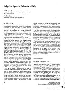
2.1. Crop water stress simulations in RZWQM2 Equipped with the DSSAT v4.0 (Decision Support System for Agrotechnology Transfer) CSM model (Jones et al., 2003) and SHAW, RZWQM2 v3.0 was used as the core executable program to determine water stress and soil water content. The CERES and CROPGRO models in DSSAT are adopted to simulate the growth of corn and soybean, respectively, where crop development is mainly governed by thermal time, or growing degree-days (GDD; Jones et al., 2003). RZWQM2 interacts with DSSAT by exchanging variables (Ma et al., 2005, 2006), and DSSAT supplies RZWQM2 with daily plant water uptake, nitrogen uptake, and plant growth variables. RZWQM2 model generates two water stress factors: the turgor factor (TURFAC) and the soil water factor (SWFAC) (Fang et al., 2014; Ritchie, 1998; Saseendran et al., 2014; Saseendran et al., 2015; Qi et al., 2016). While TURFAC is used to describe the level of plant water stress as it relates to the expansion of plant leaf cells, SWFAC is mainly related to photosynthesis and other elements of the dry matter accumulation processes. They are calculated Fig. 1. Flow chart of the proposed WS-based irrigation scheduling method. This chart shows the operational process of the proposed WS-based method, and how these steps interact with the parameters in the files (listed in the left box) of RZWQM2 model. The arrows between the RZWQM2 model box and the steps show the directions of data flow. For Colorado corn scenario, irrigation terminated after 30 days of the onset of grain filling; for Mississippi soybean scenario, irrigation was applied until maturity when water stress happened.

210


Z. Gu et al.

where

as (Fang et al., 2014; Saseendran et al., 2014, 2015; Qi et al., 2016):

SWFAC =

PWU TpSW

TURFAC =

SWFAC RWUEP1

TpSW is the Shuttleworth-Wallace potential transpiration (demand), (cm) PWU is the potential root water uptake calculated by DSSAT model (supply), (cm), and

(1)

(2)

(a) Input

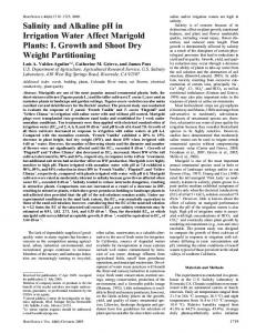
(b) Calculation Fig. 2. Interface of RZ_IrrSch using the Colorado corn scenario for 2010. (a) the parameters input interface, site-specific parameters including crop, soil and management information are automatically imported from the scenario for any modification if necessary; (b) the calculation interface, where the irrigation scheduling process will be automatically conducted according to the proposed WS-based method (Section 2.2) and provide suggestions for present day’s irrigation decision. The plot on the top of the calculation interface shows the water stress and root growth responses to a scheduled irrigation treatment during the season, while the three tables at the bottom show the scheduled irrigation events, daily main parameters (water stress, root depth, rain and suggest irrigation), and crop growth stages, respectively, from left to right.

211


Z. Gu et al.

RWUEP1 is a species-specific parameter used for evaluating water stress impact on expansion growth of cells (set at 1.5 for corn and soybean).

Pt0+ 4d is the cumulative precipitation expected for the day of irrigation and the four subsequent days (cm), Di is the depth of ith layer (cm).

In general, PWU is determined by the root length density, and the lower limit of plant-available water (i.e., the soil’s permanent wilting point, θwp ), while TpSW is dominated by weather conditions (Fang et al., 2014; Saseendran et al., 2014, 2015; Qi et al., 2016). Both SWFAC (Eq. (1)) and TURFAC (Eq. (2)) range from 0.0 (zero) for fully water stressed conditions, to 1.0 for stress-free conditions. As the value of SWFAC determined by the RZWQM2 model represents the daily crop water stress, namely the extent to which θ across the rooting depth cannot meet the crop’s transpiration demand, it provides a good indication of water deficit; accordingly, for crop water stress-based (WS-based) irrigation regime, irrigation was triggered when SWFAC dropped below 1.0.

It should be noted that the coefficient K differs in two ways from the management allowable depletion (MAD) used in ET-WB-based irrigation scheduling methods: (i) MAD defines the proportion of θfc−θwp replaced, whereas K defines the proportion of θfc−θt0 replaced, (ii) MAD acts as both the lower limit of θ at which irrigation should be triggered, and serves in computing the depth of irrigation required to restore the soil to θfc , whereas K, whose value varies just above and below 1.0, serves only to calculate the quantity of irrigation. (c) Add the irrigation event into RZWQM2 model and repeat the process daily The water input through irrigation is added to RZWQM2′s irrigation management module, then step (b) is repeated daily until a full 30 days after the onset of grain filling. Historical irrigation events of the crop season are recorded in RZWQM.DAT file which serves as an input file of RZWQM2. For corn (Zea mays L.) in RZWQM2, simulated crop yield and water stress do not response to the environment after the day of “End of grain filling” and they remain the values as those simulated on that day. In the field experiment, 43, 41, and 32 days occurred between the onset and end of grain filling in 2008, 2009 and 2010, respectively. In the field, a single irrigation event resulted in θ remaining sufficient for crop demand for about 10 days, hence simulated irrigations did not exceed 30 days after the onset of grain filling (30 days + 10 days = 40 days). If irrigation were only to end at the end of the grain filling phase, the large quantity of water then applied would likely lead to an excessively high θ , without increasing simulated crop yield. Given atmospheric conditions and soil properties at the field site, simulations on the basis of water stress, with K=1, showed irrigation water applications to rise over the season as rooting depth increased (Fig. 2b).

2.2. Crop water stress based irrigation method The WS-based irrigation scheduling drew on a calibrated RZWQM2 model was used to simulate the occurrence of water stress and then determine the quantity of water to be supplied through irrigation in order to return the current θ to θfc across the crop’s full rooting depth. Weather forecasts were downloaded from a meteorological website, allowing future precipitation to be accounted for, and thereby avoiding runoff or deep percolation arising from a full irrigation on a heavy precipitation day. The method is detailed below (Fig. 1): (a) Retrieving weather data. For real-time irrigation scheduling, historical and 4-day-ahead weather forecast data, obtained from weather websites and/or on-site weather stations, were converted to RZWQM2 weather input format. Weather data (air temperature, humidity, wind speed, precipitation and radiation) provided by CoAgMet (Ma et al., 2012b) was employed in the present study. For other applications, radiation can be calculated using the empirical equation developed by Hargreaves and Samani (1982) if it’s not provided from weather websites or on-site weather stations.

2.3. Developing the RZ_IrrSch software To facilitate the application of the proposed method, the RZ_IrrSch software was developed using Java language under the Eclipse platform. Composed of two main parts, one drawing on a weather database and another responsible for scheduling irrigation through its interaction with RZWQM2, RZ_IrrSch features a user-friendly interface created using Swing components in Java. The weather data inputs required by RZWQM2 included minimum and maximum temperature, relative humidity, wind speed, rainfall and shortwave radiation. The weather database was generated and updated by Java codes through an interaction with MySQL, a free database software provided by Oracle. For real-time scheduling the calculation of water stress requires the users to press the “Update weather” button. Upon doing so, the software reads weather data files from the on-site weather station, if available, or draws on websites for missing historical data (https://www.wunderground.com) and forecast data (http:// www.openweathermap.org). Uploaded weather data were automatically transformed to a model-specific daily format and stored in the weather database. However, in this study, the weather data being readily available, the upload and transformation steps were skipped and the original weather inputs were used instead (hmt and brk files in RZWQM2). The weather database was filled using the on-site recorded data, and the 4 days forecast precipitation was obtained from the actual historical data assuming that the 4 days’ data after the current date constituted the forecast. RZ_IrrSch provides both a parameter input interface and a calculation interface to/from the RZWQM2 model (Fig. 2). Site-specific parameters (such as crop, soil and management parameters) of user-selected RZWQM2 scenario (calibrated) were initially read by the input interface, and the scenarios named after the city nearest the field location.

(b) Determining irrigation timing and quantity based on RZWQM2 simulation. For a given day, the calibrated RZWQM2 model, drawing on readily available weather data (from step a, both historical and forecast), determined the value of SWFAC and if it was inferior to 1.0, irrigation was triggered. The quantity of water to apply was then calculated using Eq. (3). A minimum irrigation amount was required to remove the water stress on an irrigation day, in case Eq. (3) derived a small or even negative value. A minimum amount was set to 1.0 cm in this study.

IR (t0) = K {Σ(Ni = 1) (θ(fci)−θ(t(0) i) )·D(i)}−P(t0+ 4d)

(3)

where

i is the number of soil layer, N is the number of soil layer at the deepest simulated rooting depth on day t0 (cm3 cm−3), where the root depth was derived from the crop biomass. θ(fci) is the volumetric θ at field capacity of ith layer of the root zone (cm3 cm−3), θtoi is the volumetric θ of ith layer of the root zone on the day of irrigation (cm3 cm−3), K is the proportion of the deficit which is replenished, IRt0 is irrigation water supply required on the day of irrigation (t0 ) (cm),

212


Z. Gu et al.

permanent wilting point were calibrated individually in each soil layer, which can be found in Ma et al. (2012b) in detail. For the Mississippi soybean scenario, weather data including precipitation, air temperature, solar radiation, wind speed and relative humidity were obtained at Macon weather station located in Noxubee county, USA (http://ext.msstate.edu/anr/drec/stations.cgi). Noxubee county is under a humid climate with annual rainfall approximately 1400 mm, and precipitation during soybean growing season about 379 mm (Zhang et al., 2016a, 2016b). A soybean group IV cultivar was planted at 296,525 seeds per hectare on May 8, 2014 and harvested on September 10, 2014 with three irrigation treatments, which were defined as (i), ‘SM’, irrigation when measured root zone soil moisture is 50% of total plant available water and then replenish the soil to field capacity; (ii), ‘halfSM’, same irrigation timing as ‘SM’ but only provide half the amount of ‘SM’ treatment; (iii), ‘RF’, rainfed treatment without any irrigation. Soil hydraulic parameters were estimated separately in different layers according to the field experiment data. For more information about the field experiment and managements, please refer to Zhang et al. (2016a, 2016b). The simulated soybean yield of the Mississippi soybean scenario under RZWQM2 is listed in Table 1. Relative root mean square error of yield, leaf area index and soil water content are 1.35%, 13.43% and 8.86%, respectively, which is satisfactory for model calibration. Based on the above two calibrated RZWQM2 scenarios, comparisons were made between the field irrigation treatments and derived WSbased irrigation treatments from the proposed WS-based method, including simulated crop yield, soil water content and ET. The well calibrated Colorado corn scenario, which has been used in Ma et al. (2012b), was used to investigate the water saving potential, while the Mississippi soybean scenario was used to revalidate the efficiency of the proposed WS-based method. Field observed data were not used in the comparisons.

Table 1 Simulated and observed soybean yield under three field irrigation treatments. Treatments

Irrigation (cm)

Observed yield (kg ha−1)

Simulated yield (kg ha−1)

‘SM’ ‘halfSM’ ‘RF’

2.54 1.27 0

6300 6130 5930

6303 6116 5788

Note: ‘SM’ treatment means to irrigate when measured root zone soil moisture is 50% of total plant available water and then replenish the soil to field capacity; ‘halfSM’ treatment applied irrigation with the same timing as ‘SM’ but only provide half the amount of ‘SM’ treatment; ‘RF’ represents the rainfed treatment, no irrigation was applied.

The user next sets the crop planting date, and keeps parameters including crop, soil, and management information the same as the calibrated RZWQM2 model. Using the same interface, the irrigation management regime is then set to “WS-based”. The calculation interface provides users with a visual representation of changing rooting depth and water stress under the scheduled irrigation treatment. Values for water stress, irrigation quantity and timing, as well as rooting depth and rainfall, are presented in the tables below Fig. 2b. The irrigation scheduling process is initiated by clicking the “Simulation” button, the software then following the above-mentioned steps to generate a proposed regime of irrigation timing and quantity, as well as provide crop growth information (Fig. 2b). The proposed WS-based irrigation method can also be integrated in RZWQM2 model by the developers as another option for automatic irrigation scheduling like “Root Zone Depletion” and “ET Deficit”, which are already provided in RZWQM2 v3.0, however, here the developed software is additionally able to automatically convert weather data achieved from online or onsite weather stations to RZWQM2 format and visualize the scheduling process with least clicks in real time irrigation management, which is benefit for the farmers who have limited understanding of irrigation scheduling process and professional knowledge of the model.

2.5. Soil water balance equation The soil water balance equation was as follows:

2.4. The testing scenarios

P + I + SWSo = SWSe + ETa + Ds + R

(4)

where

Data from two experimental sites were employed in the evaluation of the proposed WS-based irrigation scheduling method, a Colorado corn field from Ma et al. (2012b) and a Mississippi soybean field based on data from Zhang et al. (2016a, 2016b). The Colorado corn scenario, where a full ET-WB-based irrigation schedule was applied, was calibrated and validated using data from field experiments conducted from 2008 to 2010 near Greeley, Colorado (40.45°N, 104.64°W) (Trout and Bausch, 2017; Trout and DeJonge, 2017), while the Mississippi soybean scenario was calibrated and validated using data from field experiments conducted in 2014 in Noxubee County, Mississippi in Vaiden (VA) soil type with three irrigation treatments. Both scenarios served as the basis of comparison for the present WS-based irrigation scheduling scenario. All the parameters and managements were kept unchanged when applying the calibrated scenarios, except irrigation management. For the Colorado corn scenario, weather data were recorded at a standard Colorado Agricultural Meteorological Network (http://ccc. atmos.colostate.edu/~coagmet/) weather station (GLY04). Precipitation during the growing season (from planting to harvest) was 259 mm in 2008, 244 mm in 2009 and 222 mm in 2010, which were slightly higher than the 18-year average for the location (1992–2010) from May to October (191mm). Corn (‘Dekalb 52-59′) was planted on May 12 in 2008 and May 11 in 2009 and 2010, and harvested on November 6 in 2008, November 12 in 2009 and October 19 in 2010. The mean planting density was 81000 seeds per hectare, at a row spacing of 0.76 m. Based on measured ET and water balance analysis, irrigation was applied every 3–7 days and met 100% of potential crop ET requirements (Allen et al., 1998). Water was supplied by a drip irrigation system. Soil hydraulic parameters including field capacity and

Ds is deep seepage (cm), ETa is actual evapotranspiration (cm), I is the cumulative depth of irrigation from onset to end (cm), P is the cumulated precipitation from onset to end (cm), R is run off (cm), SWSo, SWSe are the soil water storage at the onset and end of crop production, respectively (cm) 2.6. Irrigation water savings The water savings percentage was calculated as follows:

ΔI = (IF −IWS )/ IF × 100

(5)

where

ΔI is irrigation water savings percentage (%), IF is irrigation under field conditions (cm), IWS is irrigation managed under the WS-based method (cm). 3. Results and discussion 3.1. Water savings with K = 1 for Colorado corn scenarios Using a K value of 1.0, simulated crop yield under the newly developed WS-based method was similar to that the yield achieved simulated under the ET-WB-based irrigation regime (Colorado corn 213


Z. Gu et al.

scenario), where crop ET requirements were fully met. However, the WS-based irrigation regime consumed 30.5%, 17.3% and 7.1% less water than the ET-WB-based method in 2008, 2009, and 2010, respectively (Table 2). In any given year under both WS- and ET-WBbased irrigation regimes, the SWSo and P were the same, with Ds and R being relatively insignificant compared to ET or SWS. The decrease in irrigation water use under the WS-based irrigation regime (vs. the ETWB-based regime) is therefore attributable to a decrease in either ET or SWSe. In the first two years, the water savings were attributable to a decrease in both SWSe and evaporation from the soil, while in 2010 only soil evaporation showed a decrease. Plant water stress occurs when, on a daily scale, PWU < TpSW (Eq. (1)). Since when using the WS-based method for irrigation regime development, irrigation is only provided on days when PWU < TpSW , one can lower the average θ (SWS ) over the growing season (Table 2). Since the seasonal average θ decreased, Ea was lowered as well, therefore, with an irrigation regime that reduces θ after the “End of grain filling,” both Ta and SWSe could be reduced, as neither would contribute to enhancing yield. The less frequency of irrigation events under WS-based regime (Table 2), which reduced the wetting frequency of the soil surface, also contributed to the decrease of Ea. The RZWQM2 model’s output showed that the lower Ta under the WS irrigation regime with K = 1 was the result of lower transpiration after “End of grain filling” than occurred under the ET-WB regime (Table 3). Reduced Ea during the growing season, together with reducing Ta and SWS after “End of grain filling” contributes to the water saving achieved by the WS-based irrigation scheduling method here proposed. A comparison of changes in θ under the ET-WB-based irrigation regime and those under the WSbased regime (K = 1) over three years (Fig. 3), shows that the overall θ under the WS-based scheduling method was lower than that under the ET-WB-based method. The WS-based irrigation scheduling regime maintained θLL < θ < θfc , while the ET-WB- based regime could result in θ > θfc . The extra water applied under the ET-WB-based treatment was eventually stored in the soil, thereby increasing SWSe (Table 2), or wasted as excessive evaporation during the growing season or as transpiration after “End of grain filling” (Table 3). The proposed WSbased method even increased Ta during the period from planting to “End of grain filling,” thereby guaranteeing crop growth. Fereres and Soriano (2007) pointed out that when irrigation was applied at rates below ET, the crop can extract water from the soil when the historically stored soil water was sufficient to compensate the deficit and therefore the plant transpiration would not be affected, which indicates the water saving potential superior to ET-WB method. The proposed method in this study, therefore, made a full use of the soil water storage to satisfy the crop transpiration. Another study by Panigrahi et al. (2014) revealed that irrigation at 50% ETc during the early fruit growth period of ‘Kinnow’ mandarin tree would improve their water use efficiency without significantly affecting the fruit yield. Making the full use of the crop tolerance to water stress (Panigrahi et al., 2014), as well as the soil water storage (Fereres and Soriano, 2007), therefore in this work, contributed to the water-savings and

Table 3 Actual evaporation (Ea) and transpiration (Ta) before and after “End of grain filling” under ET/water balance- and water stress- (K = 1) based irrigation scheduling regimes (Colorado corn scenario). Irrigation regime

2008ET-WB 2008WS_K = 1 2009ET-WB 2009WS_K = 1 2010ET-WB 2010WS_K = 1

From planting to “End of grain filling”

From “End of grain filling” to harvest

Ea (cm)

Ta (cm)

Ea (cm)

Ta (cm)

20.1 18.8 23.5 19.9 23.0 21.1

38.8 40.4 39.7 39.7 36.1 36.5

3.6 1.0 2.6 2.1 1.0 1.1

9.0 4.0 3.1 3.1 7.0 5.8

Note: Ea: actual evaporation; Ta: actual transpiration; ET-WB: field irrigation regime based on ET and water balance; WS_K = 1: WS-based model-driven irrigation regime, where θfc is fully restored at each irrigation (K = 1).

yield maintaining. During the period from planting to harvest, Ta < TpSW , whereas from planting to “end of Grain Filling” Ta ≈ TpSW (Table 4), indicating the occurrence of water stress only after grain filling, and therefore not affecting simulated yield. Over the three years, under the WS-based irrigation scheduling regime (K=1), irrigation met crop transpiration needs before “End of grain filling,” and decreased transpiration afterwards, thereby not affecting simulated crop yield (Tables 3 and 4). An irrigation regime showing a poor potential for water savings due to timing and quantity issues would likely lead to a wide range of θ over the growing season, with θ sometimes lower than the θLL and sometimes in excess of θfc (Fig. 3). This would affect crop growth and waste irrigation water. For 2008 and 2010, a slight water stress occurred at the vegetative stage under the ET-WB-based irrigation regime, when the θ exceeded θLL (defined by MAD), and θ even exceeded on occasion since August of the three years. As the ET-WB-based irrigation regime was based on applying water to replenish a certain percentage of the previous few days’ crop ET requirements, it could fail to promptly maintain θ at an appropriate level, resulting in excessive soil water storage and increased ET after crop maturity, without, however, enhancing yield. In general, the WS-based irrigation scheduling regime saved water compared to the ET-WB-based irrigation regime by decreasing θ to such an extent that daily SWFAC or TURFAC remained above 1 over the growing season, and additionally decreasing irrigation frequency (decrease Ea), ensuring crop growth and reducing ET. As a result, irrigation demand could be decreased. 3.2. Potential water saving with K < 1 under Colorado corn scenarios Frequent irrigation treatments can decrease ET, increase WUE (Sensoy et al., 2007), and then save irrigation water (Sepaskhah and Kamgar-Haghighi, 1997). A lower compared to θfc may also benefit

Table 2 Simulated results of the ET-WB- and WS- based methods for 2008, 2009 and 2010 (from planting to harvest) under Colorado corn scenario. Irrigation Regime

SWSo (cm)

SWSe (cm)

P (cm)

I/n (cm)/(times)

Ea (cm)

Ta (cm)

ETa (cm)

Ds (cm)

TpSW (cm)

Total PWU (cm)

(cm)

Yield (kg ha−1)

(%)

2008ET-WB 2008WS_K=1 2009ET-WB 2009WS_K=1 2010ET-WB 2010WS_K=1

32.6

31.9 25.8 30.7 27.7 26.1 26.1

25.9

45.9/16 31.9/7 41.7/15 34.5/5 36.6/12 34.0/6

23.6 19.8 26.1 21.9 24.0 22.2

47.8 44.3 42.8 42.8 43.1 42.3

71.4 64.1 68.9 64.8 67.1 64.5

1.1 0.5 0.5 0.5 0.5 0.5

48.6 49.4 42.8 42.9 48.4 48.8

864.8 592.6 1014.9 613.6 627.6 426.4

37.4 32.3 36.3 33.0 34.7 33.0

10331 10325 10359 10355 8724 8713

– 30.5 – 17.3 – 7.1

34.1 34.9

24.4 22.2

Note: Runoff (R) was 0 for all simulations. SWSo, SWSe and : soil water storage at planting (onset) and harvest (end) and averaged over the period from onset to end; P: precipitation; I: irrigation; n: numbers of irrigation events; Ea: actual evaporation; Ta: actual transpiration; ETa: actual evapotranspiration; Ds: deep seepage; TpSW : Shuttleworth-Wallace potential transpiration; PWU: potential root water uptake; ΔI : irrigation water savings percentage (%) given by Eq. (5); ET-WB: field irrigation regime based on ET and water balance; WS_K = 1: WS-based model-driven irrigation regime, where θfc is fully restored at each irrigation (K = 1); values in bold are the same for each treatment in that year.

214


Z. Gu et al.

Fig. 3. Comparison of simulated soil water content (θ ) under the Colorado field irrigation management regime based on ET and water balance (ET-WB) and an irrigation regime based on proposed water stress approach and full replenishment of soil field capacity (θfc) (WS_K = 1) in 2008(I), 2009(II) and 2010(III). θ wp , soil moisture content at permanent wilting point;

θ LL , soil water content at lowest limit determined by management allowable depletion (MAD), MAD was set at 0.6. The θ , θfc and θ wp were weighted averages of the layers across root zone on that day (dynamic). The three vertical dashed lines from left to right marked the date of the onset of grain filling, 30 days of the onset of grain filling, and “End of Grain Filling”, respectively.

quantities of water applied at each irrigation are generally much greater than daily ET; and (iii) a tiny quantity of irrigation water applied on any given occasion would result in a moist shallow soil layer but drier deep soil layers, which would not prove beneficial for crop root elongation and decreasing of Ea. Even given the possible disadvantages under more frequent but smaller individual irrigations, it is still an interesting exercise to model such regimes to assess, in terms of water savings, how close to θLL the θ can be maintained without adverse effects on the crop. This can be investigated thanks to the RZWQM2 model by varying the K factor through an incremental decline from 1.0 to 0.3 (at 0.1 intervals). This

plant root growth and yield (Hu et al., 2009). Here with WS-based scheduling method, a lower θ to replenish to when irrigation was triggered, yet still met daily TpSW , would make it possible to use less irrigation water but maintain the yield. Were one able to maintain daily θ just above θLL (based on either SWFAC or TURFAC) throughout the growing season, then water demand for photosynthesis and dry matter accumulation would be guaranteed, and a minimum irrigation water input achieved. However, while this would be ideal, it would be difficult to implement in practice as: (i) rainfall would alter the balance between θt0 and, raising the former over the latter; (ii) practical irrigation management normally allows limited irrigation times and 215


Z. Gu et al.

Fig. 3. (continued)

Table 5 shows that over the years 2008, 2009, and 2010, varying K had little effect on simulated yield, decreasing it by only 0.5%, 1.7%, and 0.6% on average, respectively. Consistently over the three years, the water savings percentage (ΔI ) increases as K progressively decreased below 1.0. Given the fluctuation in the curves (Fig. 4), it is not entirely clear at what K value the ΔI peaks; therefore, a safe, conservative practice to save water and maintain yield would be to lower the quantity of irrigation at each application. However, a small value of K would increase the number/frequency of irrigations over the growing season (Table 5), and thereby risk lowering yields (explained afterwards), benefiting neither crop growth or the management of irrigation operations, therefore, a proper K value should be selected by weighing the water saving potential against the labor of irrigation management and the risk of crop yield loss. Water balance parameters are presented in Table 5.

would generate regimes gradually approaching the ideal condition of θ being just slight higher than θLL . Since water stress would not alter simulated crop yield after the end of the grain filling stage, the season’s last irrigation as scheduled by WSbased methods likely applies more water than is needed to exactly meet crop requirement before the “End of Grain Filling.” However, with limited weather forecast data the reality of real-time irrigation scheduling is that it would be hard to make the quantity of the last irrigation application exactly meet the requirement of θ > θLL before “End of grain filling” and θ < θLL after grain filling. Therefore, running the model and generating WS-based irrigation regimes over a range of K values could address the question of what regime best addressed these issues. A further constraint would be that, regardless of the calculated irrigation volume, to reflect common practice the lowest quantity of water to apply must equal or exceed 1.0 cm (drip irrigation system). 216


Z. Gu et al.

Fig. 3. (continued)

was set to 1.5 for corn, TURFAC stress would occur under a lesser degree of water depletion than the SWFAC stress used in this study. The greater TURFAC stress under the WS-based irrigation regimes where K < 1, would adversely affect the expansion of plant leaf cells, and in so doing reduce crop yield. A further modification of the proposed WSbased irrigation scheduling method based on TURFAC should be investigated. One supposes that a higher yield might be achieved with a similar amount of water by making, throughout the growing season, the daily potential root water uptake (PWU) greater than 1.5 times (for maize) the TpSW . Some ET based irrigation management practices (Sensoy et al., 2007; Wang et al., 2006) applied the same total amount of water under various irrigation frequencies, and found that the higher frequency irrigation would enhance the crop yield, which might because of the higher possibilities of removing the crop water stress under more frequent irrigation.

The WS-based irrigation regimes where K < 1 showed a greater water saving potential (vs. the ET-WB-based irrigation regime) than a WS-based regime with K = 1, which is consistent with the finding in Popova and Kercheva (2004) that irrigations scheduled at 75–80% of the required irrigation depth (K < 1) would save water and reduce drainage while insignificantly affect the yield. The percent savings in 2008, 2009 and 2010 were about 35%, 30%, and 16%, respectively, for 0.6 ≤ K ≤ 0.9, compared to 30.5%, 17.3% and 7.1% for K = 1. Simulated crop yield was not affected, with a negligible change about 0.03–3.81% decrease when K < 1, likely due to water stress towards the end of the reproductive stage, since such regimes supplied no water in the 30 days after the onset of grain filling (θ after the last irrigation event is not sufficient for crop demand extending to the “End of Grain Filling”). Another possible reason for the negligible yield decrease is the more frequent occurrence of TURFAC stress likely to occur with the increase of irrigation frequency when K < 1. As RWUEP1 in Eq. (2) 217


Z. Gu et al.

Table 4 Comparison of actual transpiration (Ta) and potential transpiration (TpSW ) for the period from plant to “End of Grain Filling” (Colorado corn scenario).

2008ET-WB 2008WS_K = 1 2009ET-WB 2009WS_K = 1 2010ET-WB 2010WS_K = 1

From Planting to Harvest

From Planting to “End of Grain Filling”

Ta (cm)

TpSW (cm)

Ta (cm)

TpSW (cm)

47.8 44.3 42.8 42.8 43.1 42.3

48.6 49.4 42.8 42.9 48.4 48.8

38.8 40.4 39.7 39.7 36.1 36.5

39.6 40.4 39.7 39.7 36.1 36.5

Note: Ta: actual transpiration;: Shuttleworth-Wallace potential transpiration; ET-WB: field irrigation regime based on ET and water balance; WS_K = 1: WS-based model-driven irrigation regime, where θfc is fully restored at each irrigation (K = 1).

3.3. WS-based irrigation method for Mississippi soybean scenario

Fig. 4. Irrigation water savings for the three years with changing coefficient K under Colorado corn scenario. K varied from 0.3 to 1.0 with an interval of 0.1. For the tested three years in Colorado, water savings percentage showed an increase trend with the decrease of the proportion K, even with some fluctuation. Yield decrease was minor under varying K.

The derived WS-based irrigation treatments under varied K (0.3–1.0) were listed in Table 6. Even though the WS-based method failed to get water saving compared to field ‘SM’ treatment, this method improved soybean yield by 291 kg ha−1 (4.6% vs. ‘SM’ treatment) on average when K varied from 0.3 to 1.0, while consumed 3.43 cm more water on average. With the decrease of K value, irrigation was applied more frequently but with less total amount of water during the growing season, and simulated yield was slightly increased by 4–5%. As the Mississippi site is located in a humid area without irrigation water scarcity, a total amount of up to 8.12 cm water supply may be worthy to obtain a higher yield. Similar to the simulated result under Colorado corn scenario, a lower K value was suggested in the irrigation management for the Mississippi site when using the proposed WS-based method to reduce water application and maintain the yield.

model must be satisfactorily calibrated according to widely used statistics (for example, with relative root mean square error less than 30%, PBIAS less than 15%), requiring accessibility to site-specific crop production data with various responses to water deficits across seasons, and accurate site-specific meteorological data (from an on-site weather station or website API). The proposed scheduling method is also seemed to be less applicable for flood or furrow irrigation than drip or subsurface irrigation. These constraints limit the agricultural regions within which this irrigation scheduling method can be applied, and the irrigated crops are limited to those in the DSSAT model integrated in RZWQM2. Furthermore, model outputs of irrigation timing and quantity do not consider the spatial variability of θ in the field. Moreover, different irrigation scheduling methods reflect different costs. The ETWB-based method needs input variables like soil type, meteorological data, phenological stage of the crop and calibration of Kc curves, along with identification of soil types (Vellidis et al., 2014, 2015). Methods based on θ or plant stress measurements are implemented through the installation of various sensors, whose measurements must also be calibrated (Cardenas-Lailhacar and Dukes, 2010; Gontia and Tiwari,

3.4. Strengths and weaknesses Water savings were achieved under a WS-based (vs. ET-WB-based) irrigation scheduling regime, while maintaining the yield (with minor decreases of 0.5%, 1.7% and 0.6% on average, under varying K for the three years, respectively) at the Colorado corn site, whereas at the Mississippi site, higher yield was achieved by consuming slightly more water. However, to make this WS-based method effective, the RZWQM2

Table 5 Parameters under WS-based irrigation treatments with variable K for 2008, 2009 and 2010 (from plant to harvest) under Colorado corn scenario. WS-based Irrigation Regime

SWSo (cm)

SWSe (cm)

P (cm)

I/n (cm) /(times)

Ea (cm)

Ta (cm)

ETa (cm)

Ds (cm) TpSW (cm)

Total PWU (cm)

(cm)

Yield (kg·ha-1)

(%)

Yield decrease (%)

2008_K = 1 2008_K = 0.9 2008_K = 0.8 2008_K = 0.7 2008_K = 0.6 2009_K = 1 2009_K = 0.9 2009_K = 0.8 2009_K = 0.7 2009_K = 0.6 2010_K = 1 2010_K = 0.9 2010_K = 0.8 2010_K = 0.7 2010_K = 0.6

32.6

25.8 25.8 25.8 25.8 25.8 27.7 25.9 25.8 25.7 25.8 26.1 26.1 26.0 26.0 26.0

25.9

31.9/7 28.7/7 29.1/8 30.5/9 29.5/10 34.5/5 29.7/5 29.1/6 27.0/6 30.0/8 34.0/6 32.4/6 31.8/7 31.1/7 27.6/8

19.8 18.6 18.8 19.3 18.8 21.9 19.7 19.7 19.1 20.1 22.2 21.8 21.5 21.0 20.0

44.3 42.3 42.5 43.5 42.9 42.8 42.1 41.5 40.1 42.0 42.3 41.2 40.9 40.7 38.3

64.1 60.9 61.3 62.7 61.7 64.8 61.8 61.2 59.2 62.1 64.5 63.0 62.4 61.7 58.3

0.5 0.5 0.5 0.5 0.5 0.5 0.5 0.5 0.5 0.5 0.5 0.5 0.5 0.5 0.5

592.6 443.3 441.4 508.4 456.5 613.6 452.7 431.8 366.2 366.3 426.4 398.6 364.4 335.9 291.8

32.3 31.4 31.4 31.7 31.5 33.0 31.9 31.7 31.3 31.5 33.0 32.7 32.5 32.3 32.0

10325 10280 10287 10316 10324 10355 10340 10356 9964 10353 8713 8706 8688 8695 8636

30.5 37.5 36.6 33.6 35.7 17.3 28.8 30.2 35.3 28.1 7.1 11.5 13.1 15.0 24.6

0.06 0.49 0.43 0.15 0.07 0.04 0.18 0.03 3.81 0.06 0.13 0.21 0.41 0.33 1.01

34.1

34.9

24.4

22.2

49.4 49.3 49.4 49.4 49.4 42.9 42.9 42.9 42.8 42.9 48.8 48.8 48.9 48.9 48.8

Note: K = 1–0.6: WS-based model-driven irrigation regime, where K times of the (θfc−θt0 ) deficit was restored at each irrigation. Runoff (R) was 0 for all simulations. SWSo, SWSe and : soil water storage at planting (onset) and harvest (end) and averaged over the period from onset to end; P: precipitation; I: irrigation; n: numbers of irrigation events; Ea: actual evaporation; Ta: actual transpiration; ETa: actual evapotranspiration; Ds: deep seepage; TpSW : Shuttleworth-Wallace potential transpiration; PWU: potential root water uptake; ΔI : irrigation water savings percentage (%) given by Eq. (5); yield decrease was expressed as a percentage compared to the yield under ET/water balance based field irrigation regime (Colorado corn scenario); values in bold are the same for each treatment in that year.

218


Z. Gu et al.

4. Conclusions

Table 6 Comparison between simulated results of the field ‘SM’ and WS-based irrigation treatments (from planting to harvest) under Mississippi soybean scenario. Irrigation regime

I/n (cm)/ (times)

‘SM’ WS_K = 1 WS_K = 0.9 WS_K = 0.8 WS_K = 0.7 WS_K = 0.6 WS_K = 0.5 WS_K = 0.4 WS_K = 0.3

2.54/1 8.12/2 7.05/2 5.99/2 5.92/3 5.86/4 4.79/4 5.00/5 5.00/5

Yield (kg ha−1)

6303 6595 6591 6594 6587 6591 6607 6594 6594

(%)

Yield increase (%)

– −219.7% −177.6% −135.8% −133.1% −130.7% −88.6% −96.9% −96.9%

– 4.63% 4.57% 4.62% 4.51% 4.57% 4.82% 4.62% 4.62%

Based on the RZWQM2 model, a water stress based method and an equipped software were developed to facilitate irrigation scheduling. This was then used for corn and soybean irrigation scheduling. The software can automatically retrieve and manage weather data (sitespecific measured or online) for use in the RZWQM2 model, and determine irrigation timing and quantity in a real-time way by detecting simulated water stress after executing the RZWQM2 model and the irrigation amount is adjusted by the forecast rainfall in the following 4 days to avoid deep seepage or runoff. Interfaces were provided by the software to help users better visualize the simulated results and more easily modify irrigation-related parameters, if necessary. The simulated water savings and yield maintenance of the proposed WS-based irrigation scheduling regime were compared to a well operated ET-WB-based regime in Colorado field (Ma et al., 2012b). The newly developed WS-based irrigation approach (under full replenishment to field capacity, i.e. K = 1) saved 30.5%, 17.3% and 7.1% in total irrigation depth in 2008, 2009 and 2010, respectively. The water savings provided by the WS-based (vs. the ET-WB-based) regime was likely attributable to a decrease in root zone θ over the growing season, which, in turn, reduced soil evaporation and soil water storage. Under the WS-based regime for Colorado scenario, higher frequency with 60% to 90% of full irrigation at each event (0.6 ≤ K ≤ 0.9) provided water savings of as much as 35%, 30%, and 16%, respectively, while negligibly decreased crop yield by 0.03–3.81%. This minor drop in yield could be attributed to the greater frequency of TURFAC (vs. SWFAC) stress triggering events, their different influence on soil water distribution in the profiles and water stress towards the end of the reproductive stage. A proper value of K should be selected in order to guarantee yield and meet practical limitations with expected water saving in the field. For the Mississippi soybean site, on average crop yield increased 291 kg ha−1 though with 3.43 cm more water consuming when K varied from 0.3 to 1.0, compared to field irrigation treatments. The decreased K values resulted in less water consumption and more efficient use of the water stored in soil profile intermittently replenished by precipitation. This study revealed that the water stress-based irrigation scheme could reduce water use and maintain crop yield in semi-arid region like Colorado, whereas in humid region like Mississippi, it could increase crop yield though consume slightly more water. In general, the novelty of this proposed water stress-based irrigation scheduling approach lies on the facts that irrigation event is triggered by crop water stress index as computed using an agricultural system model and forecast rainfall is taken into consideration when determine irrigation amount. Future work is to install this system in a field and test its effectiveness in a real world scenario or setting.

Note: ‘SM’ represents the treatment to irrigate when measured root zone soil moisture is 50% of total plant available water and then replenish the soil to field capacity; K = 1–0.3: WS-based model-driven irrigation regime, where K times of the (θfc−θt0 ) deficit was restored at each irrigation. I: irrigation; n: numbers of irrigation events; ΔI : irrigation water savings percentage (%) given by Eq. (5); yield increase was expressed as a percentage compared to the yield under ‘SM’ field irrigation regime (Mississippi soybean scenario).

2008). The costs can be high when many sensors are installed in order to take into account for field variability. The corn grain yield in Weld County, Colorado (where the experiment field is located) was obtained from the website of USDA-National Agricultural Statistics Service Colorado Field Office (2017). The observed yield of the Colorado site was 11,071 kg ha−1, 10,225 kg ha−1, and 9436 kg ha−1 in year 2008, 2009 and 2010, respectively. In 2008 and 2009, the yield of the field experiment yield was similar to the mean value in Weld County, but in 2010 it was about 3000 kg·ha-1 lower, while the reason is unknown. However, the observed weather data showed that during the main growing season (From May to October), the average air temperature was 16.4 °C, 15.2 °C, and 17.3 °C for 2008, 2009 and 2010, respectively. We speculated that the lower yield in 2010 was attributed to the higher air temperature which resulted in a much shorter grain filling duration (43, 41, and 32 days in 2008, 2009 and 2010, respectively). However, by applying the proposed WS-based irrigation scheduling method using RZWQM2 and the developed tool, we can derive a relatively reliable and accurate irrigation schedule with significant water saving while maintaining yield. No sensors are required in the field and implementation is easy thanks to a user-friendly software. Moreover, drawing on weather forecasts, this method can potentially predict the future irrigation timing and quantity, allowing farmers to prepare well in advance. In the presented simulation study, 4-day forecast precipitation was obtained from the actual historical data. However, in a real case, the weather forecast and actual weather data are not necessarily the same. No matter how much the forecasted precipitation is, the water amount applied would always range from the minimum value (set as 1.0 cm in this study) to the amount replenishing the soil layer in root zone to field capacity. When rainfall in the following 4 days is more than the forecast precipitation, deep seepage or runoff might happen due to less storage space reserved in the soil profile. However, the irrigation water supply was still reduced by subtracting the forecasted precipitation, contributing to water-saving comparing to other methods without taking future rainfall into account. When the actual rainfall is less than the forecasted precipitation, then we might apply less water on the day when water stress happened, but at least the water stress could be removed by applying even the minimum water supply (1.0 cm). And afterwards when less precipitation happened, water stress would be simulated earlier and another irrigation would be triggered. How the uncertainty of forecast weather data would affect the performance of proposed WS-based irrigation scheduling method could be addressed in future field experiments.

Acknowledgements This study was carried out during a visiting study by the senior author at McGill University and was financially supported by the China Scholarship Council (CSC) program and Xinjiang Ten Thousand Talent Program for Young Professionals. References Ahuja, L.R., Rojas, K.W., Hanson, J.D., Shaffer, M.J., Ma, L., 2000. The Root Zone Water Quality Model. Water Resources Publications LLC, Highlands Ranch CO. Alderfasi, A.A., Nielsen, D.C., 2001. Use of crop water stress index for monitoring water status and scheduling irrigation in wheat. Agric. Water Manag. 47, 69–75. http://dx. doi.org/10.1016/S0378-3774(00)00096-2. Allen, R.G., Pereira, L.S., Raes, D., Smith, M., 1998. Crop evapotranspiration-guidelines for computing crop water requirements-FAO irrigation and drainage paper 56. FAO, Rome 300, D05109. Annandale, J.G., Stirzaker, R.J., Singels, A., Van der Laan, M., Laker, M.C., 2011. Irrigation scheduling research: South African experiences and future prospects. Water SA 37 (5), 751–763. http://dx.doi.org/10.4314/wsa.v37i5.12.

219


Z. Gu et al.

Ma, L., Hoogenboom, G., Ahuja, L.R., Ascough II, J.C., Saseendran, S.A., 2006. Evaluation of the RZWQM-CERES-Maize hybrid model for maize production. Agric. Syst. 87, 274–295. http://dx.doi.org/10.1016/j.agsy.2005.02.001. Ma, L., Ahuja, L., Nolan, B., Malone, R., Trout, T., Qi, Z., 2012a. Root zone water quality model (RZWQM2): model use, calibration, and validation. Trans. ASABE 55, 1425–1446. http://dx.doi.org/10.13031/2013.42252. Ma, L., Trout, T.J., Ahuja, L.R., Bausch, W.C., Saseendran, S.A., Malone, R.W., Nielsen, D.C., 2012b. Calibrating RZWQM2 model for maize responses to deficit irrigation. Agric. Water Manag. 103, 140–149. http://dx.doi.org/10.1016/j.agwat.2011.11.005. Maier, N., Dietrich, J., 2016. Using SWAT for strategic planning of basin scale irrigation control policies: a case study from a humid region in Northern Germany. Water Resour. Manage 30, 3285–3298. http://dx.doi.org/10.1007/s11269-016-1348-0. Mancosu, N., Spano, D., Orang, M., Sarreshteh, S., Snyder, R.L., 2015. SIMETAW# - a model for agricultural water demand planning. Water Resour. Manage 30, 541–557. http://dx.doi.org/10.1007/s11269-015-1176-7. McCready, M.S., Dukes, M.D., 2011. Landscape irrigation scheduling efficiency and adequacy by various control technologies. Agric. Water Manag. 98, 697–704. http:// dx.doi.org/10.1016/j.agwat.2010.11.007. McCready, M.S., Dukes, M.D., Miller, G.L., 2009. Water conservation potential of smart irrigation controllers on St. Augustinegrass. Agric. Water Manage. 96, 1623–1632. http://dx.doi.org/10.1016/j.agwat.2009.06.007. Migliaccio, K.W., Morgan, K.T., Vellidis, G., Zotarelli, L., Fraisse, C., Zurweller, B.A., Andreis, J.H., Crane, J.H., Rowland, D.L., 2016. Smartphone apps for irrigation scheduling. Trans. ASABE 59, 291–301. http://dx.doi.org/10.13031/trans.59.11158. Migliaccio, K.W., Schaffer, B., Crane, J.H., Davies, F.S., 2010. Plant response to evapotranspiration and soil water sensor irrigation scheduling methods for papaya production in south Florida. Agric. Water Manag. 97, 1452–1460. http://dx.doi.org/10. 1016/j.agwat.2010.04.012. Moller, M., Alchanatis, V., Cohen, Y., Meron, M., Tsipris, J., Naor, A., Ostrovsky, V., Sprintsin, M., Cohen, S., 2007. Use of thermal and visible imagery for estimating crop water status of irrigated grapevine. J. Exp. Bot. 58, 827–838. http://dx.doi.org/10. 1093/jxb/erl115. Nemali, K.S., van Iersel, M.W., 2006. An automated system for controlling drought stress and irrigation in potted plants. Sci. Hortic. 110, 292–297. http://dx.doi.org/10. 1016/j.scienta.2006.07.009. O'Shaughnessy, S.A., Evett, S.R., 2010. Canopy temperature based system effectively schedules and controls center pivot irrigation of cotton. Agric. Water Manag. 97, 1310–1316. http://dx.doi.org/10.1016/j.agwat.2010.03.012. O'Shaughnessy, S.A., Evett, S.R., Colaizzi, P.D., Howell, T.A., 2011. Using radiation thermography and thermometry to evaluate crop water stress in soybean and cotton. Agric. Water Manag. 98, 1523–1535. http://dx.doi.org/10.1016/j.agwat.2011.05. 005. O'Shaughnessy, S.A., Evett, S.R., Colaizzi, P.D., Howell, T.A., 2012. A crop water stress index and time threshold for automatic irrigation scheduling of grain sorghum. Agric. Water Manag. 107, 122–132. http://dx.doi.org/10.1016/j.agwat.2012.01.018. Panigrahi, P., Sharma, R.K., Hasan, M., Parihar, S.S., 2014. Deficit irrigation scheduling and yield prediction of ‘Kinnow’ mandarin (Citrus reticulate Blanco) in a semiarid region. Agric. Water Manag. 140, 48–60. http://dx.doi.org/10.1016/j.agwat.2014. 03.018. Popova, Z., Kercheva, M., 2004. Integrated strategies for maize irrigation and fertilization under water scarcity and environmental pressure in Bulgaria. Irrig. Drain. 53, 105–113. http://dx.doi.org/10.1002/ird.104. Ritchie, J., 1998. Soil water balance and plant water stress. In: Understanding Options for Agricultural Production. Springer, Netherlands, pp. 41–54. http://dx.doi.org/10. 1002/ird.104. Saseendran, S.A., Ahuja, L.R., Ma, L., Nielsen, D.C., Trout, T.J., Andales, A.A., Chávez, J.L., Ham, J., 2014. Enhancing the water stress factors for simulation of corn in RZWQM2. Agron. J. 106, 81–94. http://dx.doi.org/10.2134/agronj2013.0300. Saseendran, S.A., Trout, T.J., Ahuja, L.R., Ma, L., McMaster, G.S., Nielsen, D.C., Andales, A.A., Chávez, J.L., Ham, J., 2015. Quantifying crop water stress factors from soil water measurements in a limited irrigation experiment. Agric. Syst. 137, 191–205. http://dx.doi.org/10.1016/j.agsy.2014.11.005. Seidel, S.J., Werisch, S., Barfus, K., Wagner, M., Schütze, N., Laber, H., 2016. Field evaluation of irrigation scheduling strategies using a mechanistic crop growth model. Irrig. Drain. 65, 214–223. http://dx.doi.org/10.1002/ird.1942. Sensoy, S., Ertek, A., Gedik, I., Kucukyumuk, C., 2007. Irrigation frequency and amount affect yield and quality of field-grown melon (Cucumis melo L.). Agric. Water Manag. 88, 269–274. http://dx.doi.org/10.1016/j.agwat.2006.10.015. Sepaskhah, A., Kamgar-Haghighi, A., 1997. Water use and yields of sugarbeet grown under every-other-furrow irrigation with different irrigation intervals. Agric. Water Manag. 34, 71–79. http://dx.doi.org/10.1016/S0378-3774(96)01290-5. Singh, A., 2010. Decision support for on-farm water management and long-term agricultural sustainability in a semi-arid region of India. J. Hydrol. 391, 63–76. http://dx. doi.org/10.1016/j.jhydrol.2010.07.006. Steppe, K., De Pauw, D.J.W., Lemeur, R., 2008. A step towards new irrigation scheduling strategies using plant-based measurements and mathematical modelling. Irrig. Sci. 26, 505–517. http://dx.doi.org/10.1007/s00271-008-0111-6. Thompson, R.B., Gallardo, M., Valdez, L.C., Fernández, M.D., 2007a. Determination of lower limits for irrigation management using in situ assessments of apparent crop water uptake made with volumetric soil water content sensors. Agric. Water Manag. 92, 13–28. http://dx.doi.org/10.1016/j.agwat.2007.04.009. Thompson, R.B., Gallardo, M., Valdez, L.C., Fernández, M.D., 2007b. Using plant water status to define threshold values for irrigation management of vegetable crops using soil moisture sensors. Agric. Water Manag. 88, 147–158. http://dx.doi.org/10.1016/ j.agwat.2006.10.007. Trout, T.J., Bausch, W.C., 2017. USDA-ARS Colorado maizewater productivity data set.

Augustin, L.K., Yagoob, A.H., Kirui, W.K., Peiling, Y., 2015. Optimal irrigation scheduling for summer maize crop: based on GIS and CROPWAT application in Hetao district; Inner Mongolia Autonomous Region, China. J. Biol., Agric. Healthcare 5 (18), 95–102. Bartlett, A.C., Andales, A.A., Arabi, M., Bauder, T.A., 2015. A smartphone app to extend use of a cloud-based irrigation scheduling tool. Comput. Electron. Agric. 111, 127–130. http://dx.doi.org/10.1016/j.compag.2014.12.021. Bellvert, J., Zarco-Tejada, P.J., Marsal, J., Girona, J., González-Dugo, V., Fereres, E., 2016. Vineyard irrigation scheduling based on airborne thermal imagery and water potential thresholds. Aust. J. Grape Wine Res. 22, 307–315. http://dx.doi.org/10. 1111/ajgw.12173. Cardenas-Lailhacar, B., Dukes, M.D., 2010. Precision of soil moisture sensor irrigation controllers under field conditions. Agric. Water Manag. 97, 666–672. http://dx.doi. org/10.1016/j.agwat.2009.12.009. Davis, S.L., Dukes, M.D., 2010. Irrigation scheduling performance by evapotranspirationbased controllers. Agric. Water Manag. 98, 19–28. http://dx.doi.org/10.1016/j. agwat.2010.07.006. Davis, S.L., Dukes, M.D., Miller, G.L., 2009. Landscape irrigation by evapotranspirationbased irrigation controllers under dry conditions in Southwest Florida. Agric. Water Manag. 96, 1828–1836. http://dx.doi.org/10.1016/j.agwat.2009.08.005. Devitt, D., Carstensen, K., Morris, R., 2008. Residential water savings associated with satellite-based ET irrigation controllers. J. Irrigat. Drain. Eng. 134, 74–82. http://dx. doi.org/10.1061/(ASCE)0733-9437(2008) 134:1(74). Dursun, M., Ozden, S., 2011. A wireless application of drip irrigation automation supported by soil moisture sensors. Scient. Res. Essays 6, 1573–1582. http://dx.doi.org/ 10.5897/SRE10.949. Emekli, Y., Bastug, R., Buyuktas, D., Emekli, N.Y., 2007. Evaluation of a crop water stress index for irrigation scheduling of bermudagrass. Agric. Water Manag. 90, 205–212. http://dx.doi.org/10.1016/j.agwat.2007.03.008. English, M.J., Solomon, K.H., Hoffman, G.J., 2002. A paradigm shift in irrigation management. J. Irrigat. Drain. Eng. 128, 267–277. http://dx.doi.org/10.1061/(ASCE) 0733-9437(2002) 128:5(267). Fang, Q.X., Ma, L., Flerchinger, G.N., Qi, Z., Ahuja, L.R., Xing, H.T., Li, J., Yu, Q., 2014. Modeling evapotranspiration and energy balance in a wheat–maize cropping system using the revised RZ-SHAW model. Agric. For. Meteorol. 194, 218–229. http://dx. doi.org/10.1016/j.agrformet.2014.04.009. Fereres, E., Soriano, M.A., 2007. Deficit irrigation for reducing agricultural water use. J. Exp. Bot. 58 (2), 147–159. http://dx.doi.org/10.1093/jxb/erl165. Flerchinger, G.N., Saxton, K.E., 1989. Simultaneous heat and water model of a freezing snow-residue-soil system: I. Theory and development. Trans. ASAE 32 (2), 565–571. http://dx.doi.org/10.13031/2013.31040. Gontia, N.K., Tiwari, K.N., 2008. Development of crop water stress index of wheat crop for scheduling irrigation using infrared thermometry. Agric. Water Manag. 95, 1144–1152. http://dx.doi.org/10.1016/j.agwat.2008.04.017. Gowda, P.H., Chavez, J.L., Colaizzi, P.D., Evett, S.R., Howell, T.A., Tolk, J.A., 2007. ET mapping for agricultural water management: present status and challenges. Irrig. Sci. 26, 223–237. http://dx.doi.org/10.1007/s00271-007-0088-6. Gutierrez, J., Villa-Medina, J.F., Nieto-Garibay, A., Porta-Gandara, M.A., 2014. Automated irrigation system using a wireless sensor network and GPRS module. IEEE Trans. Instrum. Meas. 63, 166–176. http://dx.doi.org/10.1109/TIM.2013.2276487. Haley, M.B., Dukes, M.D., 2012. Validation of landscape irrigation reduction with soil moisture sensor irrigation controllers. J. Irrigat. Drain. Eng. 138, 135–144. http://dx. doi.org/10.1061/(ASCE)IR.1943-4774.0000391. Hargreaves, G.H., Samani, Z.A., 1982. Estimating potential evapotranspiration. J. Irrigat. Drain. Divis. 108, 225–230. Hedley, C.B., Yule, I.J., 2009. A method for spatial prediction of daily soil water status for precise irrigation scheduling. Agric. Water Manag. 96, 1737–1745. http://dx.doi.org/ 10.1016/j.agwat.2009.07.009. Hoppula, K.I., Salo, T.J., 2006. Tensiometer-based irrigation scheduling in perennial strawberry cultivation. Irrig. Sci. 25, 401–409. http://dx.doi.org/10.1007/s00271006-0055-7. Hu, X.T., Chen, H., Wang, J., Meng, X.B., Chen, F.H., 2009. Effects of soil water content on cotton root growth and distribution under mulched drip irrigation. Agric. Sci. China 8, 709–716. http://dx.doi.org/10.1016/S1671-2927(08)60269-2. Idso, S., Jackson, R., Pinter, P., Reginato, R., Hatfield, J., 1981. Normalizing the stressdegree-day parameter for environmental variability. Agric. Meteorol. 24, 45–55. http://dx.doi.org/10.1016/0002-1571(81)90032-7. Jackson, R.D., Idso, S., Reginato, R., Pinter, P., 1981. Canopy temperature as a crop water stress indicator. Water Resour. Res. 17, 1133–1138. http://dx.doi.org/10.1029/ WR017i004p01133. Jones, J.W., Hoogenboom, G., Porter, C.H., Boote, K.J., Batchelor, W.D., Hunt, L., Wilkens, P.W., Singh, U., Gijsman, A.J., Ritchie, J.T., 2003. The DSSAT cropping system model. Eur. J. Agron. 18, 235–265. http://dx.doi.org/10.1016/S11610301(02)00107-7. Jones, H.G., 2004. Irrigation scheduling: advantages and pitfalls of plant-based methods. J. Exp. Bot. 55, 2427–2436. http://dx.doi.org/10.1093/jxb/erh213. Linker, R., Ioslovich, I., Sylaios, G., Plauborg, F., Battilani, A., 2016. Optimal model-based deficit irrigation scheduling using AquaCrop: a simulation study with cotton, potato and tomato. Agric. Water Manag. 163, 236–243. http://dx.doi.org/10.1016/j.agwat. 2015.09.011. Lopes, S.O., Fontes, F.A.C.C., Pereira, R.M.S., de Pinho, M., Gonçalves, A.M., 2016. Optimal control applied to an irrigation planning problem. Math. Probl. Eng. 2016, 1–10. http://dx.doi.org/10.1155/2016/5076879. Ma, L., Hoogenboom, G., Ahuja, L.R., Nielsen, D.C., Ascough II, J.C., 2005. Development and evaluation of the RZWQM-CROPGRO hybrid model for soybean production. Agron. J. 97 (4), 1172–1182. http://dx.doi.org/10.2134/agronj2003.0314.

220


Z. Gu et al.

http://dx.doi.org/10.1016/j.agwat.2005.02.016. Yuan, G., Luo, Y., Sun, X., Tang, D., 2004. Evaluation of a crop water stress index for detecting water stress in winter wheat in the North China Plain. Agric. Water Manag. 64, 29–40. http://dx.doi.org/10.1016/S0378-3774(03)00193-8. Qi, Z., Ma, L., Bausch, W.C., Trout, T.J., Ahuja, L.R., Flerchinger, G.N., Fang, Q.X., 2016. Simulating maize production, water and surface energy balance, canopy temperature, and water stress under full and deficit irrigation. Trans. ASABE 59, 623–633. http:// dx.doi.org/10.13031/trans.59.11067. Zhang, B., Feng, G., Kong, X., Lal, R., Ouyang, Y., Adeli, A., Jenkins, J.N., 2016a. Simulating yield potential by irrigation and yield gap of rainfed soybean using APEX model in a humid region. Agric. Water Manag. 177, 440–453. http://dx.doi.org/10. 1016/j.agwat.2016.08.029. Zhang, B., Feng, G., Read, J.J., Kong, X., Ouyang, Y., Adeli, A., Jenkins, J.N., 2016b. Simulating soybean productivity under rainfed conditions for major soil types using APEX model in East Central Mississippi. Agric. Water Manag. 177, 379–391. http:// dx.doi.org/10.1016/j.agwat.2016.08.022. Zotarelli, L., Dukes, M., Scholberg, J., Femminella, K., Munoz-Carpena, R., 2010. Irrigation scheduling for green bell peppers using capacitance soil moisture sensors. J. Irrig. Drain. Eng. 137, 73–81. http://dx.doi.org/10.1061/(ASCE)IR.1943-4774. 0000281.

Irrig. Sci. 35, 241–249. Trout, T.J., DeJonge, K.C., 2017. Water productivity ofmaize in the US high plains. Irrig. Sci. 35, 251–266. USDA-National Agricultural Statistics Service Colorado Field Office, 09/15/2017. Colorado Annual Agricultural Statistics Bulletin (2009-2011). < https://www.nass. usda.gov/Statistics_by_State/Colorado/Publications/Annual_Statistical_Bulletin/ index.php > . Vellidis, G., Liakos, V., Perry, C., Tucker, M., Collins, G., Snider, J., Andreis, J., Migliaccio, K., Fraisse, C., Morgan, K., 2014. A smartphone app for scheduling irrigation on cotton. In: Proceedings of the 2014 Beltwide Cotton Conference, New Orleans, LA, National Cotton Council, Memphis, TN. Vellidis, G., Liakos, V., Tucker, M., Perry, C., Andreis, J., Fraisse, C., Migliaccio, K., 2015. A smartphone app for precision irrigation scheduling in cotton, Precision agriculture'15. Wageningen Academic Publishers, pp. 713–720. http://dx.doi.org/10. 3920/978-90-8686-814-8_87. Vellidis, G., Tucker, M., Perry, C., Kvien, C., Bednarz, C., 2008. A real-time wireless smart sensor array for scheduling irrigation. Comput. Electron. Agric. 61, 44–50. http://dx. doi.org/10.1016/j.compag.2007.05.009. Wang, F., Kang, Y., Liu, S., 2006. Effects of drip irrigation frequency on soil wetting pattern and potato growth in North China Plain. Agric. Water Manag. 79, 248–264.

221