1
Development of EMD-based denoising methods inspired by Wavelet thresholding Yannis Kopsinis, Member IEEE, and Stephen (Steve) McLaughlin, Senior Member IEEE,
Abstract One of the tasks for which EMD is potentially useful is non-parametric signal denoising, an area for which wavelet thresholding has been the dominant technique for many years. In this paper, the wavelet thresholding principle is used in the decomposition modes resulting from applying EMD to a signal. We show, that although a direct application of this principle is not feasible in the EMD case, it can be appropriately adapted by exploiting the special characteristics of the EMD decomposition modes. In the same manner, inspired by the translation invariant wavelet thresholding, a similar technique adapted to EMD is developed leading to enhanced denoising performance.
Index Terms Signal denoising, Empirical Mode Decomposition, Wavelet thresholding
EDICS: DSP-WAVL I. I NTRODUCTION The Empirical mode decomposition (EMD) method [3] is an algorithm for the analysis of multicomponent signals [4] that breaks them down into a number of amplitude and frequency modulated (AM/FM) The authors are with the Institute for Digital Communications, School of Engineering and Electronics, the University of Edinburgh, Alexander Graham Bell Bldg, King’s Buildings, EH9 3JL, Edinburgh, UK, (e-mail:{y.kopsinis, Steve.McLaughlin}@ed.ac.uk). This work was performed as part of the BIAS consortium under a grant funded by the EPSRC under their Basic Technology Programme. Part of this paper has been presented in [1] and [2]. ¡b¿Copyright (c) 2008 IEEE. Personal use of this material is permitted. However, permission to use this material for any other purposes must be obtained from the IEEE by sending a request to
[email protected].¡/b¿
2
zero mean signals, termed intrinsic mode functions (IMFs). In contrast to conventional decomposition methods such as wavelets, which perform the analysis by projecting the signal under consideration onto a number of predefined basis vectors, EMD expresses the signal as an expansion of basis functions which are signal-dependent, and are estimated via an iterative procedure called sifting. Although many attempts have been made to improve the understanding of the way EMD operates or to enhance its performance (see for example [5], [6], [7], [8], [9]), EMD still lacks a sound mathematical theory and is essentially described by an algorithm. However, partly due to the fact that it is easily and directly applicable and partly because it often results in interesting and useful decomposition outcomes, it has found a vast number of diverse applications such us biomedical [10], [11], watermarking [12] and audio processing [13] to name a few. Apart from the specific applications of EMD listed above, a more generalised task in which EMD can prove useful is signal denoising. In this paper, inspired by standard wavelet thresholding and translation invariant thresholding, a number of EMD-based denoising techniques are developed1 and tested in different signal scenarios and white Gaussian noise. It is shown, that although the main principles between wavelet and EMD thresholding are the same, in the case of EMD, the thresholding operation has to be properly adapted in order to be consistent with the special characteristics of the signal modes resulting from EMD. The remainder of the paper is organised as follows: Section II provides a brief description of EMD and the notation required in the rest of the paper is also introduced. In section III the major concepts of wavelet thresholding as well as conventional EMD denoising are described. Section IV explores the possibility of adapting the wavelet thresholding principles in thresholding the decomposition modes of EMD directly. Consequently, three novel EMD-based hard and soft thresholding strategies are presented. The performance evaluation of the novel denoising techniques is illustrated in section V and the final conclusions are drawn in section VI. II. EMD: A BRIEF
DESCRIPTION AND NOTATION
Empirical mode decomposition (EMD) [3] adaptively decomposes a multicomponent signal [4] x(t) into a number L, of the so called, Intrinsic Mode Functions (IMFs), h(i) (t), 1 ≤ i ≤ L, x(t) =
L X
h(i) (t) + d(t).
(1)
i=1
1
Matlab scripts for all the novel denoising in methods developed in this paper can be downloaded from:
http://www.see.ed.ac.uk/∼ykopsini/emd/emd.html
3
where d(t) is a remainder which is a non zero-mean slowly varying function with only few extrema. Each one of the IMFs, say the ith one h(i) (t), is estimated with the aid of an iterative process, called sifting, applied to the residual multicomponent signal x(t) (i) x (t) = x(t) − Pi−1 h(j) (t) j=1
,i=1 (2) ,i≥2
The sifting process used in this study is the standard one [3]. According to this, during the (n + 1)th (i)
sifting iteration, the temporary IMF estimate hn (t) is getting improved according to the following steps2 : (i)
1) Find the local maxima and minima of hn (t). (i)
2) Interpolate, using natural cubic splines, along the points of hn (t) estimated in the first step in order to form an upper and a lower envelope. 3) Compute the mean of the two envelopes. (i)
4) Obtain the refined estimate hn+1 (t) of the IMF by subtracting the mean found in the previous step (i)
from the current IMF estimate hn (t). 5) Proceed from step 1 again unless a stopping criterion has been fulfilled. The sifting process is effectively an empirical but powerful technique for the estimation of the mean m(i) (t) of the residual multicomponent signal x(i) (t) locally a quantity that we term total local mean3 .
Although the notion of the total local mean is somewhat vague, especially for multicomponent signals, in the EMD context it means that its subtraction from x(i) (t) will lead to a signal, which is actually the corresponding IMF, i.e. h(i) (t) = x(i) (t) − m(i) (t), that is going to have the following properties: 1) Zero mean. 2) All the maxima and all the minima of h(i) (t) will be positive and negative respectively. Often, but not always, the IMFs resemble sinusoids which are both amplitude and frequency modulated (AM/FM). By construction, the number of, say N (i), extrema of h(i) (t) positioned at time instances r (i) = (i)
(i)
(i)
(i)
[r1 , r2 , . . . , rN (i) ] and the corresponding IMF points h(i) (rj ), j = 1, . . . , N (i) will alternate
between maxima and minima, i.e., positive and negative values. As a result, in any pair of extrema, (i)
(i)
(i)
(i)
r j = [h(i) (rj ), h(i) (rj+1 )], corresponds to a single zero-crossing zj . Depending on the IMF shape, 2
For the first iteration, x(i) (t) is used as temporary IMF estimate h1 (t).
3
The term local mean whould be more appropriate but we avoided here because it is usually used to describe the mean of
the two envelopes of the second step of the sifting iteration.
4
the number of zero-crossings can be either4 N (i) or N (i) − 1. Moreover, each IMF, lets say the one of order i, have fewer extrema than all the lower order IMFs, j = 1, . . . , i − 1, leading to fewer and fewer oscillations as the IMF order increases. In other words, each IMF occupies lower frequencies locally in the time-frequency domain than its preceding ones.
Fig. 1.
Empirical mode decomposition of the noisy signal shown in (a)
Fig. 1 depicts as an example the EMD of the well studied piecewise-regular signal [14] (Fig. 1a) corrupted by white Gaussian noise corresponding to 5dB signal to noise power ratio (SNR). EMD results in 10 IMFs and the final remainder, which are depicted in Fig. 1b-l. III. S IGNAL
DENOISING
Digital signal denoising can be described as follows: Having a sampled noisy signal x(t) given by x(t) = x ¯(t) + σn(t), t = 1, 2, . . . , N
(3)
where, x ¯(t) is the noiseless signal and n(t) are independent random variables Gaussian distributed N (0, 1), produce an estimate x ˜(t) of signal x ¯(t). Noise variance σ can be known or unknown and the
denoising methods can be categorised as parametric or non-parametric depending on whether a predefined parametric model of x ¯(t) has been adopted or not. In this paper, the focus is on the non-parametric 4
The end points of the signal are counted as extrema.
5
framework where the best known candidates are denoising techniques based on wavelet decomposition [14], [15], [16]. Moreover, the novelty of this paper lies in the introduction of new non-parametric thresholding techniques applied to the decomposition modes resulting from EMD instead of the wavelet components. As will be seen, thresholding in EMD, is not a straightforward application of the concepts used in wavelet thresholding. A. Wavelet based denoising Employing a chosen orthonormal wavelet basis, an orthogonal N × N matrix W is appropriately built [17] which in turn leads to the discrete wavelet transform (DWT) c = Wx
where, x = [x(1), x(2), . . . , x(N )] and c = [c1 , c2 , . . . , cN ] contains the resultant wavelet coefficients. Due to the orthogonality of matrix W , any wavelet coefficient ci follows a normal distribution with variance σ and mean the corresponding coefficient value c¯i of the DWT of the noiseless signal x ¯(t). Provided that the signal under consideration is sparse in the wavelet domain, which is usually the case, then the DWT is expected to distribute the total energy of x ¯(t) in only a few wavelet components lending themselves to high amplitudes. As a result, the amplitude of most of the wavelet components is attributed to noise only. The fundamental reasoning of wavelet thresholding is to set to zero all the components which are lower than a threshold related to the noise level, i.e., T = σC , where C is a constant, and then reconstruct the denoised signal x ˜(t) utilising the high amplitude components only. There are two major thresholding operators: hard and soft thresholding defined by: y, |y| > T ρT (y) = 0, |y| ≤ T, and
respectively.
sgn(y)(|y| − T ), |y| > T ρT (y) = 0, |y| ≤ T,
(4)
(5)
Using any one of the thresholding operators above, the estimated denoised signal is given by ˜ = WT˜ x c
(6)
where, c˜ = [ρT (c1 ), ρT (c2 ), . . . , ρT (cN )] and W T denotes transposition of matrix W . Apart from the standard wavelet thresholding described above, a number of modifications are investigated in our
6
simulation results section including translation invariant thresholding [14], and Bayesian-based wavelet thresholding [18], [15].
√ With respect to the threshold selection, the universal threshold T = σ 2 ln N is a popular candidate.
Such a threshold guarantees with high probability that all of the components attributed to noise will have lower amplitudes. In this paper, multiples of the above threshold are used and the standard deviation of the noise is estimated using a robust estimator based on the components median [14]: σ ˆ=
median(|ci | : i = 1, . . . , N ) 0.6745
(7)
The specific standard deviation estimator leads to accurate estimates even if there are components attributed to signal. Finally, it is usually beneficial to apply thresholding after a primary resolution level leaving the coarse scales corresponding to low frequencies unthresholded. This parameter will be also taken into account in our study. Wavelet hard thresholding 40 15.6468 20 0 -20 (a) Wavelet translation-invariant thresholding 40 16.7123 20 0 -20 (b) Wavelet Bayesian thresholding 40 17.8156 20 0 -20 0
Fig. 2.
1000
2000 (c)
3000
4000
Examples of Wavelet-based denoising when SNR=5dB. The top-left numbers are the SNR values after denoising.
Fig. 2a-c shows the noise-free estimates of the signal of Fig. 1a corrupted by noise using, from top to bottom, wavelet hard thresholding with universal threshold, translation invariant wavelet thresholding with universal threshold and Bayesian-based wavelet thresholding. The numbers on the top left of the figures indicate the SNRs after the denoising procedure when the SNR is 5dB before denoising. Note that this performance corresponds to a single arbitrary noise realisation. Detailed, ensemble averaged performance results of the thresholding techniques above will be presented in section V.
7
B. Conventional EMD denoising The first attempt at using EMD as a denoising tool emerged from the need to know whether a specific IMF contains useful information or primarily noise. Thus, significance IMF test procedures were simultaneously developed both by Flandrin et. al. [5], [19] and Wu et. al. [20], [21] based on the statistical analysis of modes resulted from the decomposition of signals solely consisting of fractional Gaussian noise and white Gaussian noise respectively. The reasoning underlying the significance test procedure above is fairly simple but strong. If the energy of the IMFs resulting from the decomposition of a noise-only signal with certain characteristics is known, then in actual cases of signals comprising both information and noise following the specific characteristics, a significant discrepancy between the energy of a noise-only IMF and the corresponding noisy-signal IMF indicates the presence of useful information. In a denoising scenario this translates to partially reconstructing the signal using only the IMFs which contain useful information and discarding the IMFs that carry primarily noise, i.e., the IMFs that share similar amounts of energy with the noise-only case. In practice the noise-only signal is never available in order to apply EMD and estimate the IMF energies, so the usefulness of the above technique relies on whether or not the energies of the noise-only IMFs can be estimated directly based on the actual noisy-signal. The latter is usually the case due to a striking feature of EMD. Apart from the first noise-only IMF, the power spectra of the other IMFs exhibit self similar characteristics akin to those which appear in any dyadic filter structure. As a result, the IMF energies, Ek , should linearly decrease in a semi-log diagram of, e.g., log2 Ek with respect to k for k ≥ 2. It also turns out that the first IMF carries the highest amounts of energy. In this paper the
focus is on signals with white Gaussian noise. Then, the noise-only IMF energies can be approximated [19] according to equation: 2 ˆk = E1 ρ−k , k = 2, 3, 4, . . . E β
(8)
where, E12 is the energy of the first IMF and β , ρ are parameters which, for a specific EMD implementation, depend mainly on the number of sifting iterations used. These parameters can be estimated in one step based on a large number of independent noise realisations and their corresponding IMFs [19]. Fig. 3 shows the curves that link the estimated energies of the IMFs k = 1, . . . , 10, based on model (8), where the parameters β and ρ correspond to EMDs using from 1 up to 15 sifting iterations. We observe that as the number of sifting iterations increases, the corresponding curves approach each other. This is in agreement with the analytically derived frequency responses of the equivalent filtering operations that correspond to EMDs with different number of sifting iterations in a two sinusoids signal case [6].
8 8
6
4
2
15 siftings
0
1 sifting
-2
Flandrin et al
-4
-6 1
2
3
4
5
6
7
8
9
10
IMF # Fig. 3. Curves that link the estimated energies of the IMFs which correspond to EMDs using from 1 up to 15 sifting iterations. The thick red line indicated as “Flandrin et al” corresponds to the β and ρ parameters proposed in [19].
Flandrin et al [19] specifically proposed for the parameters β and ρ parameters the values 0.719 and 2.01 respectively, that correspond to the curve drawn with thick red line. We see that these parameters correspond to a curve which is representative by being close to an average of the “trend” that the rest of the energy curves exhibit. Hereafter, the IMF energy curve that corresponds to the later specification of β and ρ will be called fixed in order to coincide with the sifting dependent IMF energy curves.
Fig. 4. (a) Theoretical noise-only model and actual IMF energies with respect to IMF number. (b) The resulted denoised signal when, for the reconstruction, the IMFs number 6 to number 11 are used only.
Fig. 4 depicts the conventional denoising procedure and results when it is applied on the test signal of
9
Fig. 1a. On top, with solid line we see the semilog diagram (energies with respect to IMF number) of the corresponding IMFs (Fig. 1b-l) and the dashed line shows the results of the noise only model of (8). We observe, after the fifth IMF the energies significantly diverge from the theoretical model indicating the presence of significant amounts of no-noise signal. The partial signal reconstruction including only IMF number 6 to 11 results in the denoised signal shown in Fig. 4. IV. IMF
THRESHOLDING - BASED DENOISING
In this paper an alternative denoising procedure inspired by wavelet thresholding is proposed. Some preliminary results have already appeared very recently in [22], [23], [24] where the wavelet thresholding idea is directly applied to the EMD case. However, as will be seen later, EMD-thresholding can exceed the performance achieved by wavelet thresholding only by adapting the thresholding function to the special nature of IMFs. EMD can be interpreted as a subband like filtering procedure resulting in essentially uncorrelated IMFs. Although the equivalent filter-bank structure is by no means pre-determined and fixed as in wavelet decomposition, one can in principle perform thresholding in each IMF in order to locally exclude low energy IMF parts which are expected to be significantly corrupted by noise. A direct application of wavelet thresholding in the EMD case translates to: h(i) (t), |h(i) (t)| > T i (i) ˜ h (t) = 0, (i) |h (t)| ≤ Ti ,
(9)
for hard thresholding, and to
sgn(h(i) (t))(|h(i) (t)| − Ti ), |h(i) (t)| > Ti ˜ (i) (t) = h 0, |h(i) (t)| ≤ Ti ,
(10)
˜ (i) (t) indicates the ith thresholded IMF. The for soft thresholding where, in both thresholding cases, h
reason for adopting different thresholds Ti per mode i will become clearer in the sequel. A generalised reconstruction of the denoised signal is given by x ˆ(t) =
M2 X
k=M1
˜ (i) (t) + h
L X
h(i) (t)
(11)
k=M2 +1
where, the introduction of parameters M1 and M2 gives us flexibility on the exclusion of the noisy low order IMFs and on the optional thresholding of the high order ones which in white Gaussian noise conditions contain little noise energy.
10
There are two major differences, which are interconnected, between wavelet and direct EMD thresholding (EMD-DT) shown above. First, in contrast to wavelet denoising where thresholding is applied to the wavelet components, in the EMD case, thresholding is applied to the N samples of each IMF which are basically the signal portion contained in each adaptive subband. An equivalent procedure in the wavelet method would be to perform thresholding on the reconstructed signals after performing the synthesis function on each scale separately. Secondly, as a consequence of the first difference, the IMF samples are not Gaussian distributed with variance equal to the noise variance as the wavelet components are irrespective of scale. In fact, the noise contained in each IMF is coloured5 having different energy in each mode. In that sense, EMD denoising is most closely related to wavelet denoising of signals corrupted by coloured noise where the thresholds have to be scale dependent. In our study of thresholds, √ multiples of the IMF dependent universal threshold, i.e., Tk = C Ek 2 ln N , where C is a constant are used. Moreover, the IMF energies can be computed directly based on the variance estimate of the first IMF using (8).
A. Thresholding adapted to EMD characteristics The direct application of wavelet like thresholding, either hard or soft, to the decomposition modes is in principle incorrect and can have catastrophic consequences for the continuity of the reconstructed signal6 . This is because the IMFs resemble an AM/FM modulated sinusoid with zero mean. As a result, (i)
(i)
it is guaranteed that, even in a noiseless case, in any interval z j = [zj
(i)
zj+1 ], the absolute amplitude
of the ith IMF, i = 1, 2, . . . , N , will drop below any non-zero threshold in the proximity of the zero(i)
crossings zj
(i)
and zj+1 . In other words, based on the absolute amplitude of isolated IMF samples it is
impossible to infer for any one of them if they correspond to noise or to useful signal. However, it is (i)
possible to guess if the interval z j is noise-dominant or signal-dominant based on the single extrema (i)
h(i) (rj ) that correspond to this interval. If the signal is absent, the absolute value of this extrema will
lie below the threshold. Alternatively, in the presence of strong signal, the extrema value can be expected to exceed the threshold. Moreover, since in each IMF the noise and the signal share the same bandwidth, the signal dominance at the extrema time instance is highly likely to be extended to all the IMF samples 5
There is strong evidence that at least in the noise-only case the distribution of the IMF samples is still Gaussian [21].
6
The denoising procedure used in [11] differs from direct thresholding since the parts of the IMFs that contain useful signal
are detected with the aid of a fractal dimension filter and consequently some of the inherent disadvantages of direct EMD thresholding can be avoided to some extent. However, this method is only efficient in denoising transient signals.
11
belonging to the specific zero-crossing interval. As a result the newly developed EMD hard thresholding, hereafter referred to as EMD interval thresholding (EMD-IT) translates to: h(i) (z (i) ), |h(i) (r (i) )| > T i j j (i) (i) ˜ h (z j ) = (i) 0, |h(i) (r )| ≤ T , j
(i)
(12)
i
(i)
(i)
(i)
for j = 1, 2, . . . , Nz , where, h(i) (z j ) indicates the samples from instant zj to zj+1 of the ith IMF. After careful consideration, it can be seen that the above procedure resembles wavelet thresholding more than direct EMD thresholding, because wavelet thresholding is applied to the wavelet coefficients. In fact, each coefficient is responsible for the values of a sequence of samples of the subsignal corresponding to the specific scale reconstruction which increases with scale and it is determined by the wavelet size of support. Similarly, the number of IMF samples which are altered or not in the EMD-IT depends on the IMF order and increases as the order increases. IMF before and after thresholding 10 0 -10
(a)
(b1)
(b3)
(b2) EMD denoising with Direct Thresholding
40 15.113 20 0 -20 (c) EMD denoising with Interval Thresholding 40 17.027 20 0 -20 0
Fig. 5.
1000
2000 (d)
3000
4000
Difference between Direct and Interval thresholding and the corresponding denoised signals.
Fig. 5a shows the difference between the direct and the interval EMD thresholding. As an example, the sixth IMF of the signal shown in Fig. 1 has been used. The thick light-colored line corresponds to the
12
actual IMF and the solid and dotted lines are associated with interval thresholding and direct thresholding respectively. The horizontal lines indicate the plus and minus of the universal thresholding.A detail of the thresholding function applied on the IMF segment between the two vertical dashed lines in Fig. 5a is also depicted in Fig. 5b1-b3. More specifically, in Fig. 5b2 and b3 we see the parts of the IMF segment which are non zero after thresholding. Clearly, EMD-DT introduces discontinuities which can be effectively reduced by the use of EMD-IT. Fig. 5c and d show the denoising effect when the two EMD-based thresholding methods are applied on the same noise realisation of the piecewise-regular signal used in Fig. 2. We observe that EMD-IT results in higher SNR than EMD-DT. In both cases, the universal threshold is adopted which, it should be noted, is not optimum; neither for EMD nor for wavelet thresholding as will become apparent in the simulations section. In a similar manner to the hard interval thresholding case, the extremum between each zero-crossing (i)
(i)
interval [zj zj+1 ] will be the processing element of reference for the case of soft iterval thresholding as well. Practically, the result of wavelet soft thresholding on, e.g. positive wavelet components that exceed the threshold is that the latter get reduced by an amount equal to the threshold. With respect to iterative soft thresholding all the IMF samples that correspond to zero-crossing interval with extremum exceeding the threshold have to be reduced in a smooth way in order for the extremum to get reduced exactly by an amount equal to the threshold. Mathematically, the described soft thresholding operation yelds: (i) (i) )|−Ti (i) h(i) (z (i) ) |h (rj (i) , |h(i) (rj )| > Ti j (i) (i) (i) h (rj )| ˜ h (z j ) = (13) (i) 0, |h(i) (rj )| ≤ Ti , B. Iterative EMD interval-thresholding Inspired by translation invariant wavelet thresholding, where a number of denoised versions of the signal under consideration are obtained iteratively in order to enhance the tolerance against noise by averaging them, we make an attempt to develop EMD-based denoising techniques which exploit a similar principle. Once again, the direct application of translation invariant denoising to the EMD case will not work. This arises from the fact that the wavelet components of the circularly shifted versions of the signal correspond to atoms centered on different signal instances. In the case of the data-driven EMD decomposition, the major processing components, which are the extrema, are signal dependent leading to fixed relative extrema positions with respect to the signal when the latter is shifted. As a result, the EMD of shifted versions of the noisy signal corresponds to identical7 IMFs sifted by the same amount. 7
The IMFs can potentially be slightly different at the boundaries but only due to edge effects associated with the spline
interpolation procedure.
13
Consequently, noise averaging cannot be achieved in this way. The different denoised versions of the noisy signal in the case of EMD can only be constructed from different IMF versions after being thresholded. Inevitably, this is possible only by decomposing different noisy versions of the signal under consideration itself. So the problem at hand translates to the following question: In which way, having a signal buried in noise, can you produce different noisy versions of the actual noise-free signal. The answer stems from within the EMD concept exploiting the characteristics of the first IMF. We know that in white Gaussian noise conditions, the first IMF is mainly noise, and more specifically comprises the larger amount of noise compared to the rest of the IMFs. By altering in a random way the positions of the samples of the first IMF and then adding the resulting noise signal to the sum of the rest of the IMFs we can obtain a different noisy-version of the original signal. In fact, in the case where the first IMF consists of noise only, then the total noise variance of the newly generated noisy-signal is the same as the original one. The above EMD denoising technique, hereafter refered to as Iterative EMD interval-thresholding (EMDIIT) is summarised in the following steps: 1) Perform an EMD expansion of the original noisy signal x. 2) Perform a partial reconstruction using the last L − 1 IMFs only, xp (t) = (1)
PL
(i) i=2 h (t).
3) Randomly alter the sample positions of the first IMF, ha (t) = ALTER(h(1) (t)). (1)
4) Construct a different noisy version of the original signal, xa (t) = xp (t) + ha (t). 5) Perform EMD on the new altered noisy signal xa (t). 6) Perform the EMD-IT denoising (Eq. 12 or 13) on the IMFs of xa (t) to obtain a denoised version x ˜1 (t) of x.
7) Iterate K − 1 times between steps 3-6 , where K is the number of averaging iterations in order to obtain k denoised versions of x, i.e., x ˜1 , x ˜2 , . . . , x ˜K . P K 1 ˜(t) = K ˜k (t). 8) Average the resulted denoised signals x k=1 x The altering function can take several forms leading to a number of modified EMD-IIT denoising schemes. In this paper we consider four different approaches: •
Random circulation: The samples of the first IMF are circularly shifted randomly.
•
Random permutation: The samples of the first IMF randomly change positions.
Fig. 6a-b shows two different noisy versions of the piecewise-regular signal obtained by the method described in the current section when the hard EMD-IT thresholding is used. In both cases, random permutation was used as a signal altering function. The denoised signals that result from 4 and 20
14
Noised version of the Piece-Regular signal 40 20 0 -20 (a) Noised version of the Piece-Regular signal 40 20 0 -20 (b) EMD denoising with Iterative Interval Thresholding (4 Iterations) 40 20 0 -20
17.1649
(c) EMD denoising with Iterative Interval Thresholding (20 Iterations) 18.0902 40 20 0 -20 0 1000 2000 3000 4000 (d) SNR w.r. to the number of Iterations 19 18 17 0
Fig. 6.
5
10 (e)
15
20
Two noisy versions of the piecewise-regular signal (a, b) and result of the EMD-based iterative interaval thresholding
method using 4 (c) and 20 (d) iterations. (e) shows the achieved SNR w.r. to the number of iterations.
iterations K , of EMD-IIT together with the achieved SNRs are illustrated in Fig. 6c and 6d respectively. The noisy signal used was that described in Fig. 5. Apparently, the proposed iterative procedure has enhanced the denoising capabilities of EMD. For completeness, Fig. 6e shows the increment in SNR of the denoised signal with respect to the number of iterations.
C. Clear Iterative EMD interval-thresholding When the noise is relatively low, enhanced performance compared to EMD-IIT denoising can be achieved with a variant called clear iterative interval-thresholding (EMD-CIIT). The need for such a modification comes from the fact that the first IMF, especially when the signal SNR is high, is likely to contain some signal portions as well. If this is the case, then by randomly altering its sample positions, the information signal carried on the first IMF will spread out contaminating the rest of the signal along
15
its length. In such an unfortunate situation, the denoising performance will decline. In order to bypass this disadvantage of EMD-IIT it is not the first IMF that is altered directly but the first IMF after having all the parts of the useful information signal that it contains removed. The “‘extraction” of the information signal from the first IMF can be realized with any thresholding method, either EMD-based or waveletbased. It is important to note that any useful signal resulting from the thresholding operation of the first IMF has to be summed with the partial reconstruction of the last L − 1 IMFs. More specifically, the steps 2 and 3 of EMD-IIT have to be replaced with the following 4 steps: 1) Perform an EMD expansion of the original noisy signal x. ˜ (1) (t) of 2) Perform a thresholding operation to the first IMF of x(t) to obtain a denoised version h h(1) (t). (1)
˜ (1) (t) 3) Compute the actual noise signal that existed in h(1) (t), hn (t)=h(1) (t) − h
4) Perform a partial reconstruction using the last L − 1 IMFs plus the information signal contained P (i) ˜ (1) in the first IMF, xp (t) = L i=2 h (t) + h (t). (1)
(1)
5) Randomly alter the sample positions of the noise-only part of the first IMF, ha (t) = ALTER(hn (t)). EMD CIIT (4 Iterations) 17.5353
40 20 0 -20
(a) EMD CIIT (20 Iterations) 18.4334
40 20 0 -20 0
19
1000
2000 (b)
3000
4000
SNR w.r. to the number of Iterations
18 17 0
Fig. 7.
5
10 (c)
15
20
Denoised signals obtained with the aid of EMD-CIIT after 4 and 20 iterations (a,b). (c) shows the achieved SNR w.r.
to the number of iterations.
The effectiveness of the subtraction from the first IMF of any existing information signal is shown in Fig. 7. For the first IMF denoising (see step 2 above), Bayesian wavelet thresholding was used. In
16
fact, in all the cases we have tested, the EMD interval thresholding performed similarly or worse than the Bayesian wavelet denoising when it came to the denoising of the first IMF. As a result, hereafter, whenever the EMD-CIIT is used, the adoption of the Bayesian method for the extraction of the useful signal from the first IMF is implied unless the use of a different method is explicitly mentioned. Fig. 7a-c illustrates the same quantities as illustrated in previous result figure and corresponds to the same noise realization with the Fig. 6c-e. The denoised signals that result from 4 and 20 iterations K of the EMDCIIT together with the achieved SNRs are illustrated in Fig. 7c and 7d respectively. The noisy signal used was the same as in Fig. 5. The proposed iterative procedure has enhanced the denoising capabilities of EMD. In both cases, random permutation was used as a signal altering function. For completeness, Fig. 7e shows the increment in SNR of the denoised signal with respect to the number of iterations. V. S IMULATION
RESULTS
Apart from the piecewise-regular signal three more representative test signals shown in Fig. 8a-c have been used for validation of the proposed denoising techniques. Moreover, the best of the methods have been applied two real signals, a call signal from a bat belonging to the species Pipistrellus Pygmaeus8 shown in Fig. 8d and a speech signal segment illustrated in Fig. 8e. To start with, the effect on the denoising performance of either adopting fixed or sifting dependent IMF energy curves with respect to the number of sifting iterations is studied in Fig. 9. More specifically, the adopted performance measure is the SNR after denoising when the SNR before denoising is either 0dB (Fig. 9a,c) or 15dB (Fig. 9b,d) and the signals used are the Piece-wise regular and the Doppler signal (Fig. 8a) both sampled with sampling frequency that result in 2048 samples. The results shown correspond to ensemble average of 50 independent noise generalizations. The dashed curves correspond to the EMD-IT method and the solid curves to EMD-CIIT and the crosses and the squares correspond to fixed and sifting dependent IMF energy curves respectively. A number of conclusions can be drawn. First, when the signal is regular such as the Doppler one, the larger the number of sifting iterations then the better the performance is. In contrast, when the signal has irregularities, e.g., the Piece-regular signal case, the best performance (especially in the iterative EMD-CIIT method) is achieved with a relatively low number of sifting iterations. These results have been evaluated with other regular and irregular signals. In general, a balanced trade off between number of sifting and performance is realized with about 8 8
This
bat-call
was
provided
by
Dr
(http://www.fbs.leeds.ac.uk/staff/profile.php?tag=Waters)
Dean
Waters
of
the
University
of
Leeds
17
Doppler Signal
(a) Blocks Signal
(b) Bumps Signal
(c) Bat-call Signal
(d) Speech Signal
(e)
Fig. 8.
Some of the signals used for validation of the denoising methods.
Piece-wise Regular, SNR=0dB
Doppler, SNR=0dB
Piece-wise Regular, SNR=15dB
15.5
Doppler, SNR=15dB
28
25 EMD-IT EMD-CIIT EMD-IT variable EMD-CIIT variable
SNR after denoising
13.3
27
15
24.5
26
13.2
14.5
24
25
13.1
13 0
23.5
5
Fig. 9.
10 Siftings (a)
15
20
23 0
14
EMD-IT EMD-CIIT EMD-IT variable EMD-CIIT variable
5
10 Siftings (b)
15
20
13.5
EMD-IT EMD-CIIT EMD-IT variable EMD-CIIT variable
0
5
10 Siftings (c)
15
EMD-IT EMD-CIIT EMD-IT variable EMD-CIIT variable
24
20
23 0
5
10 Siftings (d)
15
SNR after denoising with respect to the number of sifting iterations in the cases of fixed or sifting dependent IMF
energy curves.
20
18
sifting iterations. Second, it is apparent that the sifting dependent IMF curves do not offer significant advantages over the fixed one since the performance difference never exceeds 0.2 dB. In addition, the sifting dependent curves can even lead to slight performance deterioration in the case of EMD-CIIT when the signal has both intense irregularities and a small number of sifting iterations are used. This happens because in this case it is very likely that large information signal portions (in the places where the irregularities exist) get extracted in the first IMF compromising the iterative thresholding operation. For the rest of the simulation examples, each one of the artificial test signals is sampled and tested with four different sampling frequencies to generate four versions per signal having 1024, 2048, 4096 and 8192 samples. As before, the results shown correspond to ensemble average of 50 independent noise generalizations and in all EMD-based denoising methods the number of sifting iterations was fixed and equal to 8. The adoption of a fixed number of sifting iterations may result in modes which do not comply with the IMF characteristics. More specifically, it is possible to find two or even more maxima (or minima) between neighboring zero-crossings. In such cases, the thresholding is naturally performed based on the largest (smallest) value of the maxima (minima) lying between consecutive zero-crossings. Moreover, the adopted performance measure is the SNR after denoising which corresponds to SNR values of 0, 5, 10 and 15 dB before denoising. The performance results for all different methods shown correspond to hard thresholding. The conclusions drawn from the hard thresholding denoising are in general valid for the soft thresholding variants and a discussion on the later type of thresholding can be found at the end of the section. 35
30
30
SNR after denoising
35
35
30
25 25
25 20
20
20 15 15
1024
2048
4096
# of samples (a)
Fig. 10.
8192
1024
2048
4096
# of samples (b)
EMD-IIT (p) EMD-CIIT (p) EMD-IIT (c) EMD-CIIT (c)
15
EMD-IT EMD-conv EMD-DT EMD-CIIT (p)
10
Hard-T Hard TI Bayesian
8192
1024
2048
4096
# of samples (c)
Performance evaluation of the Doppler signal using wavelet and EMD-based denoising methods.
Next, a thorough denoising performance evaluation of the developed and wavelet-based methods is realised using the Doppler signal (Fig. 8a) and then the performance of the best of the techniques when
8192
19
applied on the rest of the signals is examined. Fig. 10a-c depicts the performance comparison between wavelet techniques, existing and newly developed EMD-based techniques and variants of denoising methods based on the iterative interval thresholding principle respectively. In each graph, the performance curves correspond to SNR after denoising versus number of signal samples and they are grouped in 4 sets associated with 15dB SNR before denoising (dashed-dotted curves), 10dB SNR (dotted curves), 5dB SNR (solid curves) and 0dB SNR (dashed curves). The results of the wavelet-based techniques are shown in Fig. 10a. We observe that the best performance is achieved with the translation invariant thresholding algorithm (Hard-TI) with the Bayesian technique to follow. It is clear that the performance discrepancy between Hard-TI and Bayesian increases as the initial signal SNR increases. This trend and performance order is in general common to the rest of signals tested. With respect to existing and newly developed EMD-based methods (Fig. 10b) worse performance is exhibited by the conventional denoising approach (EMD-conv). The interval thresholding (EMD-IT) leads to a 1dB improvement over direct thresholding (EMD-DT) and the incorporation of clear iterative interval thresholding with permutation altering (EMDCIIT (p)) offers about 2 dB of extra gain. Finally, the performance of several iterative interval (EMD-IIT) and clear iterative interval thresholding (EMD-CIIT) variants is shown in Fig. 10c with the number of iterations being fixed to 20. It would appear that the different methods perform in a similar way, with the EMD-CIIT denoising performing the best especially in the case of high SNR (10dB and 15dB) and low number of samples (1024 and 2048). Moreover, the random permutation methods slightly outperform the random circulation ones. The effect of the altering method can be further investigated with the aid of Fig. 11 where the performance of the IIT and CIIT methods when applied to the 2048 samples Doppler signal is displayed with respect to the number of iterations. We observe that in all the cases the random circulation altering method exhibits a much faster performance improvement with respect the number of iterations compared to random permutation. However, random permutation outperforms the random circulation after about 9 or 18 iterations in the cases of IIT or CIIT respectively. This result appears unexpected at first glance. The first IMF is roughly concentrated in the upper half band of the spectrum and consequently one would expect that the averaging procedure would perform best when the altered IMFs occupy the same frequencies with the original IMF. However, this is only true for the circulation altering function. In contrast, the permutation altering inevitably leads to the redistribution of the IMF energy over the whole band. As a result, when random permutation is adopted, the denoising problem can be considered more demanding in the sense that the noise contained in the different noisy versions of the signal under consideration is no longer white. We feel that a possible explanation for the improved performance that
20
the permutation-based denoising exhibits over the circulation-based approach, would be the effect that the perturbation has on the information signal which is contained in the first IMF. In general, the energy of the signal portions existing in the first IMF will be concentrated in time. This is true since the reason that the part of a signal is in the first IMF is its high frequency and/or high energy. This requirement is likely to be fulfilled at time intervals rather than time instances. As a result, the perturbation function will effectively spread the energy of the information signal along the full time axis reducing its destructive effect. Indeed, the improvements achieved with the perturbation altering method are more profound in the EMD-IIT case where the first IMF is not cleared from the information signal residual.
26
SNR=15 dB 25
~ ~
~ ~
15
14
EMD-IIT (c)
SNR=0 dB
EMD-CIIT (c) EMD-IIT (p) EMD-CIIT (p)
13 0
Fig. 11.
2
4
6
8
10
12
14
16
18
20
Study of effect of the first IMF altering method.
Based on the results above, the techniques which are going to be used for a comparative performance study discussed next are the EMD-IIT and EMD-CIIT both using random permutation altering representing the EMD-based methods and the Hard-TI and Bayesian representing the wavelet-based methods. Fig. 12a-c shows the corresponding performance curves related to the Doppler, the piecewise-regular and the blocks signals. It can be observed that the EMD-based methods outperform the Bayesian method for all the combinations of signal number of samples and signal SNR used. Moreover, the translation invariant hard thresholding method exhibits a significant performance improvement in the cases that the noise is relatively low (15dB SNR) outperforming both the Bayesian and the EMD-based methods. Moreover, we see that in general the improvement of the EMD-based methods with respect to the increment of the sampling frequency is higher than the improvement of the Hard-TI method. As a result, even in 15dB SNR the performance of the EMD denoising techniques tends to reach the high
21 Doppler Signal
Piece-Regular Signal
30
26
25
25
22
20
20
18
15
15
1024
2048
4096
EMD-IIT (p) EMD-CIIT (p) Hard-TI Bayesian 8192
10
14
1024
# of samples (a)
Blocks Signal
30
30
2048
4096
EMD-IIT (p) EMD-CIIT (p) Hard-TI Bayesian 8192 1024
2048
# of samples (b)
4096
EMD-IIT (p) EMD-CIIT (p) Hard-TI Bayesian 8192
# of samples (c)
Fig. 12. Performance evaluation of EMD and wavelet-based denoising methods applied on the Doppler, piecewise-regular and blocks signals.
performance levels of Hard-TI. A counter example to this is the bumps signal (Fig. 8c) where Hard-TI Bumps Signal
30
25
SNR after denoising
SNR after denoising
35
20
15
10
1024
EMD-IIT (p) EMD-CIIT (p) Hard-TI Bayesian 2048
4096
8192
# of samples Fig. 13.
Performance evaluation of EMD and wavelet-based denoising methods applied to the bumps signal.
outperforms the rest of the methods in all the SNRs tested with the exception of the 8192 samples case where the EMD-CIIT method performs the best as seen in Fig. 13. Another measure which characterises the performance of the denoising methods is the variance of the SNR estimates, resulting from many realizations, which is shown in Table I for all the artificial signals tested with 2048 samples and for two
22
SNR values (0dB and 15dB). The EMD-CIIT method exhibits quite a low variance, in a manner similar to the Bayesian method in contrast to the Hard-TI which results in higher variances and sometimes double that of the other methods. This is considered as an advantage of the EMD-CIIT based methods9.
Method EMD-CIIT (p) Hard-TI Bayesian
Doppler 0 dB 15 dB 0.3888 0.2319 0.8173 0.4909 0.4358 0.2532
Piece-Regular 0 dB 15 dB 0.2437 0.1694 0.4396 0.2510 0.3199 0.1787
Blocks 0 dB 0.2107 0.2821 0.1722
Bumps 15 dB 0.0953 0.1732 0.1334
0 dB 0.1798 0.1887 0.1511
15 dB 0.1184 0.0946 0.1012
TABLE I
Speech
Bat-call
VARIANCE OF
Methods
-2 dB EMD-CIIT (c) 8.443/0.066 EMD-CIIT (p) 8.449/0.066 Hard-TI 7.311/0.053 Methods
-2 dB EMD-CIIT (c) 9.504/0.061 EMD-CIIT (p) 9.504/0.061 Hard-TI 8.316/0.058
THE
0 dB 10.009/0.055 10.018/0.056 9.747/0.055 0 dB 10.704/0.046 10.705/0.046 9.842/0.036
SNR S OF THE DENOISED SIGNALS .
SNR/Variance 2 dB 5 dB 11.649/0.05 14.145/0.05 11.659/0.05 14.156/0.05 11.651/0.06 14.354/0.062 SNR/Variance 2 dB 5 dB 11.932/0.033 13.718/0.021 11.934/0.033 13.725/0.021 11.283/0.028 13.285/0.027
10 dB 18.235/0.021 18.271/0.02 20.307/0.043
15 dB 21.413/0.022 21.527/0.023 23.664/0.034
10 dB 17.061/0.02 17.088/0.02 16.523/0.017
15 dB 20.730/0.017 20.764/0.017 20.263/0.014
TABLE II SNR PERFORMANCE AND VARIANCE OF EMD AND
WAVELET- BASED DENOISING METHODS APPLIED ON BAT AND SPEECH SIGNAL .
The SNR of the denoised bat and the speech signal of Fig. 8d-e together with the corresponding variances are shown in Table II. With respect to the bat-call signal, the EMD-based methods outperform Hard-TI only for low SNR values. In the case of the speech segment signal EMD denoising leads to gains between 1 to 0.5 dB compared to the Hard-TI method irrespectively of the noise level. Note that the sampling frequency of these signals is fixed in advance. 9
EMD-IIT methods result in somewhat higher variances.
23
In all of the above simulations, the SNR values shown correspond to optimized values for the several parameters that each method use such as the primary resolution level for the wavelet based denoising techniques and parameters M1 , M2 of equation (11) for the EMD based denoising. With respect to M1 , an appropriate choice stems from the lower order IMF which contains significant portions of useful signal as it is computed by conventional EMD denoising [19] . If for example according to the conventional EMD approach the denoised signal has to be formed as the reconstruction of the IMFs of order J and higher (for example J = 6 in Fig. 4), then it has been empirically found that a very good choice of M1 is given by M1 = max(1, J − 2)
(14)
On the other hand, a good choice of M2 is L−2. In other words, the last two IMFs do not get thresholded. However, M2 can be practically set to zero without significant effect on the performance. Finally, for the methods that thresholding is applied to, the best among the 11 thresholds was adopted for each one of the different SNR/sampling frequency simulation setups. The 11 thresholds were calculated by multiplication of the universal threshold with the constants 0.4 up to 1.4 with steps of 0.1; It appears that in the vast majority of simulation examples and all the different simulation setups, the best threshold for the EMD-based methods was found to be between 0.6 to 0.8 times the universal threshold with a small performance discrepancy for any threshold between the above values. The picture is similar in the case of translation invariant thresholding with the difference that the optimum threshold values were between 0.8 and 0.9 times the universal threshold. Based on the specific signals tested we did not observe any noticeable increase in the sensitivity on the accuracy of the threshold selection of the EMD denoised techniques over the wavelet-based methods
SNR after denoising
Piece-Regular Signal 28
24
26
22
24
20
22
18
20
16
18
14
16
12
14
10
Soft EMD-CIIT (c) Soft EMD-CIIT (p) Soft thresholding Soft-TI
8 6 -2
0
2
4
6
8
10
SNR before denoising (a)
Fig. 14.
Doppler Signal
26
12
14
12
Soft EMD-CIIT (c) Soft EMD-CIIT (p) Soft thresholding Soft-TI
10 8 16 -2
0
2
4
6
8
10
12
14
16
SNR before denoising (b)
Performance evaluation of EMD-base and wavelet-based soft thresholding techniques.
In Fig. 14 the performance of the EMD-CIIT method when it incorporates soft thresholding is compared
24
with the performance of the ordinary and the translation invariant wavelet based soft thresholding methods when applied to the piecewise-regular and the Doppler signal. The simulations are repeated for two different sampling frequencies leading to 1024 (dashed curves) and 4096 (solid curves) samples. Firstly, we observe that in the case of soft thresholding the soft-TI exhibits inferior performance compared to standard soft thresholding. Second, the EMD methods outperform the wavelet thresholding ones for all of the tested SNRs. However, the trend observed in the hard thresholding case, namely that some of the wavelet based methods reach and even outperform the EMD methods is still present. When soft thresholding is used, the optimum thresholds are smaller than in the case of hard thresholding. More specifically, the EMD-CIIT methods have to use thresholds close to 0.3-0.4 times the universal threshold while the wavelet methods perform best with thresholds close to 0.5-0.6 times the universal threshold. Moreover, parameter M2 plays a more important role when soft thresholding is adopted. This is a result of the way that soft thresholding operates and the fact that the optimized thresholds are quite small, the thresholding of the high order (low frequency) IMFs can possibly lead to a power reduction of useful signal portions. As a result it is wise to set parameter M2 to much higher values than in the hard thresholding case, e.g. to set M2 to 5 or even higher. In the SNR results of Fig. 14 parameter M2 was not optimized but was fixed at 5. VI. C ONCLUSIONS In this paper, the principles of hard and soft wavelet thresholding including translation invariant denoising were appropriately modified in order to develop denoising methods suited for thresholding EMD modes. The novel techniques presented exhibit an enhanced performance compared to wavelet denoising in the cases where the signal SNR is low and/or the sampling frequency is high. These preliminary results suggest further efforts for improvement of EMD-based denoising when denoising of signals with moderate to high SNR would be appropriate. R EFERENCES [1] Y. Kopsinis and S. McLauglin, “Empirical mode decomposition based soft-thresholding,” in 16th European Signal Processing Conference - EUSIPCO, 2008. [2] Y. Kopsinis and S. McLauglin, “Empirical mode decomposition based denoising techniques,” in 1st IAPR Workshop on Cognitive Information Processing - CIP, 2008. [3] N. E. Huang et. al., “The empirical mode decomposition and the hilbert spectrum for nonlinear and non-stationary time series analysis,” Proc. R. Soc. Lond. A, vol. 454, pp. 903–995, Mar. 1998. [4] L. Cohen, Time-Frequency Analysis, Prentice Hall, 1995.
25
[5] P. Flandrin, G. Rilling, and P. Goncalves, “Empirical mode decomposition as a filter bank,” IEEE Signal Processing Lett., vol. 11, pp. 112– 114, Feb. 2004. [6] G. Rilling and P. Flandrin, “One or two frequencies? the empirical mode decomposition answers,” IEEE Trans. Signal Processing, pp. 85–95, Jan. 2008. [7] Y. Washizawa, T. Tanaka, D. P. Mandic, and A. Cichocki, “A flexible method for envelope estimation in empirical mode decomposition,” in Knowledge-Based Intelligent Information and Engineering Systems, 10th International Conference, KES 2006, Bournemouth, UK, 2006. [8] Y. Kopsinis and S. McLauglin, “Investigation and performance enhancement of the empirical mode decomposition method based on a heuristic search optimization approach,” IEEE Trans. Signal Processing, pp. 1–13, Jan. 2008. [9] Y. Kopsinis and S. McLauglin, “Improved EMD using doubly-iterative sifting and high order spline interpolation,” EURASIP Journal on Advances in Signal processing, vol. 2008, Article ID 128293, 8 pages, 2008. [10] Y. Zhang, Y. Gao, L. Wang, J. Chen, and X. Shi, “The removal of wall components in doppler ultrasound signals by using the empirical mode decomposition algorithm,” IEEE Trans. Biomed. Eng., vol. 9, pp. 1631–1642, Sept. 2007. [11] L. Hadjileontiadis, “Empirical mode decompostion and fractal dimension filter,” IEEE Eng. Med. Biol. Mag., pp. 30 – 39, Jan. 2007. [12] B. Ning, S. Qiyu, Y. Zhihua H. Daren, and H. Jiwu, “Robust image watermarking based on multiband wavelets and empirical mode decomposition,” IEEE Trans. Image Processing, pp. 1956 – 1966, Aug. 2007. [13] Md. K. I. Molla and K. Hirose, “Single-mixture audio source separation by subspace decomposition of hilbert spectrum,” IEEE Trans. on Audio, Speech and Language Processing, pp. 893 – 900, Aug. 2007. [14] S. Mallat, A wavelet tour of signal processing, Academic press, second edition, 1999. [15] A. Antoniadis and J Bigot, “Wavelet estimators in nonparametric regression: A comparative simulation study,” Journal of statistical software, vol. 6, pp. 1–83, 2001. [16] D. L. Donoho and I. M. Johnstone, “Ideal spatial adaptation by wavelet shrinkage,” Biometrika, vol. 81, pp. 425–455, 1994. [17] S. Theodoridis and K. Koutroumbas, Pattern Recognition, Academic press, third edition, 2006. [18] H. C. Huang and N. Cressie, “Deterministic/stochastic wavelet decomposition for recovery of signal from noisy data,” Technometrics, vol. 42, pp. 262–276, 2000. [19] P. Flandrin, G. Rilling, and P. Gonc¸alv`es, EMD equivalent filter banks, from interpetation to applications (in N. E. Huang and S. Shen, Hilbert-Huang Transform and Its Applications), World Scientific Publishing Company, first edition, 2005. [20] Z. Wu and N. E. Huang, “A study of the characteristics of white noise using the empirical mode decomposition method,” Proc. Roy. Soc. London A, vol. 460, pp. 1597–1611, June 2004. [21] N. E. Huang Z. Wu, Statistical significance test of intrinsic mode functions, (in N. E. Huang and S. Shen, Hilbert-Huang Transform and Its Applications), World Scientific Publishing Company, first edition, 2005. [22] A. O. Boudraa and J. C. Cexus, “Denoising via empirical mode decomposition,” in ISCCSP2006, 2006. [23] Y. Mao and P. Que, “Noise suppression and flaw detection of ultrasonic signals via empirical mode decomposition,” Russian Journal of Nondestructive Testing, vol. 43, pp. 196–203, 2007. [24] T. Jing-tian, Z. Qing, T. Yan, L. Bin, and Z. Xiao-kai, “Hilbert-huang transform for ECG de-noising,” in 1st International Conference on Bioinformatics and Biomedical Engineering (ICBBE 2007), 2007.