Nov 20, 1995 - Cryptography is used to encode the secret transactions of banks, governments, .... The greatest common divisor of this list is 2, a factor of 22.
Quantum-inspired computing Mark Moore and Ajit Narayanan Department of Computer Science Old Library University of Exeter Exeter EX4 4PT UK November 20, 1995 Abstract
The paper identi es and demonstrates the feasibility of a novel computational paradigm which is inspired by the principles of quantum mechanics and quantum computing. A brief history of quantum computing and basic exposition of quantum mechanics are provided, followed by a detailed description of Shor's quantum `algorithm' for factoring very large numbers. An extension to Shor's method is described, and this leads to two further applications of `quantum-inspired' methods: sorting, and the 15-puzzle. In all cases, quantum-inspired methods require the use of `classical' methods to determine whether the candidate answers provided by the quantum-inspired methods are correct. Finally, some basic methodological principles and guidelines are provided for quantum-inspired computing. The aim is not to provide a formal exposition of quantum-inspired computing but to identify its novelty and potential use in tackling NP-hard problems.
1
1 Introduction It has been estimated that every two years for the past 50 years computers have become twice as fast while their components have become twice as small [Lloyd, 1995]. If progress continues at this rate future computer circuits will be based on nanotechnology1 and the behaviour of such circuits will have to be given in quantum mechanical terms rather than in terms of classical physics, since on the atomic scale matter obeys the laws of quantum mechanics. Richard Feynman [Feynman, 1982, Feynman, 1986] showed how a quantum system could be used to perform computations and could act as a simulator for probabilistically weighted quantum processes, where such simulations are impossible to achieve e�ciently on a conventional probabilistic or non-deterministic automaton. This is because such simulations on a `classical' non-deterministic TM involve an exponential growth in the number of computational steps at each branch in the weighted probabilistic space. In the case of the quantum TM, quantum parallel computation implies that we can e�ciently compute a partial solution within each path of an exponentially branching space in a way that cannot be easily simulated classically. This suggests that the computational power of a quantum computer can exceed that of a classical one | not in what can be computed but in the e�ciency of computation. The universal TM U [Turing, 1936] is the most general possible classical computer, and all general purpose computers are approximations to it. U can simulate any Turing machine with perfect precision, where a TM in turn is a theoretical model that can simulate the execution of a single algorithm on a classical computer. Deutsch [Deutsch, 1985] showed that a universal quantum computer Q can perfectly simulate any TM and can also simulate any quantum computer or simulator with arbitrary precision. Quantum computers cannot compute a function that is not Turing-computable, but they do give new methods of computation for many classes of problem. A theory of quantum computational networks which is a generalisation of the theory of quantum logic gates is also described [Deutsch, 1989], thereby grounding such networks in future developments in nanotechnology, where the operation of nano-devices will be best (and perhaps only) described at the quantum level. Deutsch [Deutsch, 1985, Deutsch, 1989] also showed that any physical process could be modelled perfectly on a quantum computer, and that such a computer would be able to perform tasks more quickly than traditional machines. This, he argued, was because the quantum machines would be able to exploit the phenomenon of quantum parallelism, where such machines compute each polynomial path in NP (non-deterministic polynomial) space in parallel. This implies that a quantum computer could behave as a massive parallel processing machine which explores each path of an NP-complete or NP-hard problem in polynomial time. There is one major limitation to this idea: it is not possible to observe the results of each computational path separately as they are all in di�erent universes. If an observation is made, the universes collapse to one universe, and the results in the other universes are lost. Computational techniques which aim to explore quantum parallelism must come up with observation methods which ensure that the universe which is collapsed into on observation somehow `represents' a solution to the problem. As well as these theoretical developments, claims have also been made recently [Shor, 1994] that polynomial quantum computing algorithms exist for problems (e.g. factoring of large integers into primes, discrete logarithms) which are considered non-polynomial (i.e. NP-hard) on classical computers. It is clear that the work described by Shor represents a signi cant advance in our knowledge of how to program quantum computational networks, if and when they exist.2 The aim of this paper is to examine whether there is anything that `classical' computer scientists can learn from the debate currently underway on the subject of quantum computation. First, Shor's quantum `solution' to the factoring problem is described. It is shown that the method3 em-
1 Nano = 10?9 , i.e. devices which are billionths of a metre large and work in billionths of a second. One nanometre is roughly the size of 10 atoms. 2 There is disagreement on whether quantum computers can ever be built, because of their susceptibility to noise caused by thermal vibrations and construction faults [Landauer, 1995]. 3 Strictly speaking, it cannot be called an `algorithm' since it is not guaranteed to halt or return the right results when it does halt, as will be seen later.
2
bodies some general principles which, if adopted by classical computer scientists, can o�er a novel computational framework for solving problems which are deemed to be NP-hard. These principles are abstracted from the quantum factoring domain and implemented in two other domains which can also be NP-hard in the classical sense: sorting, and determining whether a solution can be reached from an initial problem con guration. From these application domains, a general set of design and development principles has evolved for use by classical computer scientists when attempting to formulate what we call `quantum-inspired' methods for speci c problems. The term `quantum-inspired' is used deliberately to distinguish `pure' quantum computation, which is rmly based and grounded in the principles and concepts of quantum mechanics, and useful and practical computational methods which are inspired by such principles and concepts.4 Quantum-inspired computing is characterised by: 1. the use of a `quantum-inspired' computational method which is inspired by certain principles of quantum mechanics, such as standing waves, interference and coherence; and 2. the use of a classical algorithm for checking that the `candidate' solutions generated by the quantum-inspired computational method are in fact correct.
2 Basic principle of quantum mechanics The nucleus of an atom contains particles called protons (positively charged) and neutrons (electrically neutral). The nucleus is surrounded by electrons (negatively charged), and if there is an equal number of orbiting electrons and nucleus protons the atom is neutrally charged. However, the orbits of electrons, according to quantum mechanics, is not planar, in the way that the Earth's (slightly elliptical) orbit around the sun is planar. Instead, the orbit of electrons is best described as a wave (Figure 1). There are several di�erent types of orbit, depending on the angular momentum and energy level. An electron `jumps' orbit from an orbit with low energy level to an orbit with high energy level by absorbing energy (e.g. a photon). The term `quantum' signi es that there can be no in-between states or orbits. The jumps are discrete, and there are 6 energy levels which can be roughly characterised as the number of cycles an electron has to go through while orbiting the nucleus at that energy level (i.e. an electron with energy level 1 orbits the nucleus with one cycle, energy level 2 with two cycles, and so on). An electron can jump, again discretely, back to a lower energy level by releasing energy (a photon). Hence, an electron jumps states in discrete quanta by absorbing energy or releasing it. Heisenberg's uncertainty principle states that both the position and the momentum of an electron cannot be known. This is because in the act of measuring, some energy must be focused on the particle (e.g. a photon from a laser). The energy of the photon can be absorbed by the measured particle, sending it into a di�erent orbit. Hence, if the measurement shows where the particle is (and the more precise the measurement the more focused the measuring photon must be), in this very process the momentum of the particle can be altered. A quantum particle's location can best be described by a quantum state vector j , a weighted sum which in the case of two possible locations equals jA + jB , where and are complex number weighting factors of the particle being in locations A and B, respectively, and where jA and jB are themselves state vectors [Penrose, 1994]. For possible states, there will be di�erent complex number weighting factors, each describing the weighted probability of the particle being at that location.5 j represents a linear superposition of the particle given >
w
w
>
x
>
>
x
>
w
x
n
n
>
4 This is similar to connectionist networks being inspired by concepts in neurophysiology, such as layered networks of neurons, connectivity, activation and inhibitionof neighbouringneurons and signalling [Narayanan, 1990], genetic algorithms by concepts of mutation, crossover, populations and tness, and cellular automata by the way individual cells form `tissues' which at a global level perform computations which cannot be predicted from the behaviour of individual cells. 5 The weighting factors are used in ratios to calculate the probability of the particle being at A compared with that of it being at B. They are not the probabilities themselves.
3
nucleus
electron's orbit around the nucleus Figure 1: An electron's orbit is not planar but is best described as a wave. In the gure, the electron's orbit is such that it goes through one complete `cycle' around the atom, starting at some point in front of the nucleus, going around the back (dotted line) before completing its cycle. An electron orbiting a nucleus jumps states in discrete quanta (up to six) by absorbing energy or releasing it. The orbits of electrons are described by standing waves: unlike a planet orbiting the sun in a at ellipse, an electron's stable orbit takes the form of a wave. An electron at the rst quantum level oscillates one full cycle before returning to its start position, at the second level two full cycles, and so on. Energy is not produced or absorbed during an orbit but only on jumping orbits: increased oscillation requires increased energy, reduced oscillation produces energy. individual quantum state vectors.6 However, in the act of observing a quantum state (or wave function), it collapses to a single state.7 Another important principle for quantum computing concerns a particular interpretation of Thomas Young's famous `double-slit' experiment in 1801. Imagine that a photon is red at a screen which has two parallel slits and behind which there is a detector. If only one slit is open, the pattern of photons arriving at the detector is as expected if photons are discrete particles. If both slits are open, however, the pattern of arriving photons takes a wave pattern (Figure 2), resulting in alternating bright and dark regions. The interpretation of the wave pattern is that one part of the wave pattern of the photon went through one slit and the other part through the other slit, and the location of the photon on the detector is determined by how and where the two waves interfere with each other when they reach the detector. The path di�erences between the slits and the detector result in constructive and destructive interference. In this case, the photon as wave has gone through both slits. Similarly, a particle the position of which is given by two state vectors A and B is said to be at A and B at the same time. This is the `many universes' interpretation [Everett, 1957]: we must imagine all quantum systems exist in parallel universes. When a single photon passes through the two slits, the photon passes through the rst slit in one universe, and through the second slit in another universe. The limitation is that the photon cannot be viewed in the di�erent universes. To determine the position of the photon as it arrives on the screen, a measurement is made. This measurement causes the universes to interfere with each other, and yields the photon's position. The `many universes' interpretation is used by Shor in his quantum computing method for extracting prime factors of very large integers, where a memory register is placed in a superposition of all possible integers it can contain, followed by a di�erent calculation being performed in each If there are locations as given by state vectors, the particle is said to be at all locations at the same time. Although the introduction here has concentrated on electrons, the principles of quantum mechanics apply to molecules, atoms, electrons, protons, neutrons, photons, quarks and all other subatomic particles. 6 7
n
n
n
4
photon gun
P1
P2
P1 and P2 (wave)
slit 1 open slit 2 closed
slit 1 closed slit 2 open
slit 1 open slit 2 open
slit 1
slit 2
screen
detector
number of photons arriving at the detector
Figure 2: A diagram of Young's double-slit experiment. Photons are red individually from a `photon gun', through a screen with two slits, onto a detector. The pattern of photons detected when only one slit is open follows a probability distribution expected of discrete particles (white and black dots for slit 1 being open and slit 2 being open, respectively). However, when both slits are open, the pattern obtained follows a typical interference pattern obtained with waves and is not the sum of P1 and P2. Since it cannot be determined which slit a photon goes through in this case, the photons are shaded grey. `universe' (path after slit). The computation halts when the di�erent universes `interfere' with each other because repeating sequences of integers (standing waves) are found in each universe and across universes. Although there is no guarantee that the results are correct, a subsequent check can be made at this point to identify whether the numbers returned are indeed prime factors of the given large integer.
3 Quantum factoring
3.1 RSA-129
Cryptography is used to encode the secret transactions of banks, governments, and the military. The encryption method widely employed is a DES (data encryption standard) based on RSA. RSA is named after its inventors Ronald Rivest, Adi Shamir, and Leonard Adleman [Rivest et al., 1978] and is a public key encryption system.8 The success of RSA depends on the seeming intractability 8 Brie y, two distinct large prime numbers are chosen randomly, and . Their product = � is calculated. A large integer is chosen that is relatively prime to ( ? 1) � ( ? 1); is the encryption key. The decryption key is the unique multiplicative inverse of mod ( ? 1) � ( ? 1), i.e. � = 1 mod ( ? 1) � ( ? 1). (the original product) and are published in the public domain, but is kept private. For a secret communication from X to Y: X encrypts the message using Y's public key; only Y's private key is able to decrypt the message. For a signed communication from X to Y: X encrypts the message using X's private key; Y will use X's public key to decrypt the message. For a secret and signed message from X to Y, X uses X's private key then Y's public key, and Y must p
e
d
p
e
e
p
q
q
d
5
q
r
p
q
e
d
e
;
p
q
r
of the problem of nding the prime factors of very large integers. When the system was invented back in 1977 its inventors challenged anyone to factorise a particular 129-digit number, now known as RSA-129. This challenge stood until 1994, when 1600 computers linked via the Internet were able to determine the factors in just over eight months. Despite this breakthrough, cryptographers reassured themselves with the thought of adding more digits to their codes. The problem of factoring numbers becomes exponentially harder the larger they are. However, Shor [Shor, 1994] outlined a quantum algorithm that would factorise RSA-129 in a few seconds, if we could build a quantum computer that ran as fast as a modern PC.
3.2 Shor's quantum method for factorising
To factor a number (the product of two primes), specify an arbitrary number of parallel universes (0, 1, 2, ...), and randomly select an integer between 0 and . Then, in every universe, raise to the power of the number of the universe. Divide by and store the remainder in the universe. For the next number in the sequence for a universe, is raised to the power of the number last stored, divided by , and the remainder stored. This continues in each universe to form a repeating sequence. For the sake of exposition, let (the number to be factored into prime factors) be 33. Let = 7 (0 ) and = 17. Table 1 provides a detailed description of what happens in each universe 0 to 16. Consider 2 and 5: n
p
x
n
x
n
x
n
n
x
< x < n
u
p
u
u
: : 2: 3: 4: 5: 6: 7: 8: 9: 10 : 11 : 12 : 13 : 14 : 15 : 16 :
u0 u1 u u u u u u u u u u u u u u u
u
1 7 16 13 25 10 4 28 31 19 1 7 16 13 25 10 4
7 28 4 13 10 1 25 31 7 19 7 28 4 13 10 1 25
28 31 25 13 1 7 10 7 28 19 28 31 25 13 1 7 10
31 7 10 13 7 28 1 28 31 19 31 7 10 13 7 28 1
7 28 1 13 28 31 7 31 7 19 7 28 1 13 28 31 7
28 31 7 13 31 7 28 7 28 19 28 31 7 13 31 7 28
31 7 28 13 7 28 31 28 31 19 31 7 28 13 7 28 31
7 28 31 13 28 31 7 31 7 19 7 28 31 13 28 31 7
Table 1: 17 universes for identifying the prime factors of 33, given = 7. x
2 : 72 5 u5 : 7
mod 33 = 16, 716 mod 33 = 4, 74 mod 33 = 25, 725 mod 33 = 10, 710 mod 33 = 1, etc. mod 33 = 10, 710 mod 33 = 1, 71 mod 33 = 7, 77 mod 33 = 28, 728 mod 33 = 31, etc. The frequency of repeat across universes, which we call vertical frequency , , is 10, and this can be seen if we examine 0 and 10, 1 and 11, 2 and 12, and so on. That is, in each of these universes the repeating frequency starts at the same point and repeats the same numbers. While other universes share the repeating pattern, they do not share the common starting point. This is the quantum computation equivalent of standing waves in each universe: a repetition of numerical values. We now perform the calculation vf=2 ? 1, where is the arbitrarily chosen number between 0 and and is the frequency of common repeating patterns across universes. This gives us 710=2 ? 1(mod 33), which is 9.9 Now, nding the greatest common divisor of 9 and 33 gives one of the factors, i.e. 3. u
vf
u
u
u
u
u
x
n
vf
use Y's private key then X's public key to reconstruct the message. 9 75 ? 1 = 16806; 16806 mod 33 = 9.
6
u
x
Shor's method is not guaranteed to always work, and if the derived number turns out not to be a prime factor of , the procedure is repeated using a di�erent . It is claimed that on average only a few trials will be required to factorise , even when is very large. So although there are no known fast classical algorithms for factorising large numbers into primes, Shor's method uses known fast algorithms for taking a candidate prime factor of and determining whether it is in fact a prime factor. Shor's method has been extended by Moore [Moore, 1995] to deal with factoring large even numbers and squares. n
x
n
n
n
3.3 Moore's extension to Shor's method
The following sequence of steps can lead to the identi cation of factors for large even numbers and squares. 1. Initially determine the frequency of repeat in the rst universe, 0 (Table 1), in this case 3 (i.e. it takes three numbers 7, 28 and 31 before the pattern repeats. Call this (horizontal frequency). 2. However, before the repeating sequence occurs there is an introductory period consisting of numbers, in this case one (the `1' before 7, 28, 31, 7...). Calculate as + , in this case 3+1=4. 3. Now the vertical frequency of repeat is identi ed, , in this case 10. 4. If ? 2 2 � then becomes 2 � , otherwise remains + 1. In our case, 10 ? 2 8, so = 4. 5. If is odd add 1, otherwise do nothing. In our case, remains 4. 6. Create an empty list . Initialise = 0. 7. Repeat (a) Take the rst integer in universe k , calculate the absolute value of subtracting from it the rst integer in universe k+f , and append it to . In our case (Table 1), with = 0 initially and = 4, in 0 the rst integer is 1 and in k+f , i.e. 4, the rst integer is 25, and 24 is appended to , i.e. (24). (b) = + 1. 8. Until = ? 1 (i.e. goes from 0 to 9 in our example). In our example, the following individual values are obtained: abs( 0 : 1 ? 4:25) = 24; abs( 1 : 7 ? 5:10) = 3; abs( 2 : 16 ? 6:28) = 12; the seven subsequent values are 15, 6, 9, 3, 21, 15, 6. 9. Calculate the greatest common divisor of the list = (24 3 12 15 6 9 3 21 15 6). For this list = 3 (a factor of 33). This shows that Moore's extension can still be used to identify prime factors. Table 2 and Table 3 provide examples of Moore's extension working on even numbers and squares, respectively. For even numbers (Table 2), assume = 22 (the even number to be factored) and = 7 (an arbitrary number between 0 and ). The method within each universe is the same as before. Consider 1 and 4 (Table 2). 1 : 71 mod 22 = 7, 77 mod 22 = 17, 717 mod 22 = 17, etc. 4 : 74 mod 22 = 3, 73 mod 22 = 13, 713 mod 22 = 13, etc. We then have = 1 (the horizontal frequency is 1, as 17 is the only element in the recurring cycle of the rst universe, 0 ); = 2 (the introductory period before 17 begins recurring is 2 numbers long, as 1 and 7 precede the cycle); = 10 (the vertical frequency is 10, as all the values in every tenth universe are identical); and = 3 ( = + = 3). As ? 2 2 � , = 2 � , which becomes 6. As is even, we do not add 1 to its value. The following list of values is then obtained: ( 0 : 1 ? 6 : 15) = 14; u
hf
i
f
hf
i
vf
vf
>
f
f
f
f
hf
>
f
f
f
L
k
u
u
f
L
k
u
u
u
L
k
k
k
vf
u
k
u
u
u
u
L
;
u
;
;
;
;
;
;
;
;
gcd
n
x
n
u
u
u
u
hf
u
vf
f
f
hf
i
vf
>
f
f
f
f
abs u
7
u
i
( 1 : 7 ? 7 : 17) = 10; the eight subsequent values (for = 10) are 4, 6, 2, 14, 10, 4, 6, 2. The greatest common divisor of this list is 2, a factor of 22. For square numbers (Table 3), assume = 25(5 � 5) and = 13. The method within each universe is as before. This gives us = 2 (the horizontal frequency is 2, as 2 and 19 are the only two elements in the recurring cycle in the rst universe, 0); = 4 (the introductory period before 2 and 19 begin recurring is four elements long, as 1, 13, 3, and 22 precede the cycle); = 20 (the vertical frequency is 20 as all the values in every twentieth universe are identical); and = 12 ( = + = 6; as ? 2 2 � , = 2 � = 12; as is even, we do not add 1 to its value). The following list is obtained: ( 0 : 1 ? 12 : 6) = 5; ( 1 : 13 ? 13 : 3) = 10; subsequent values are 5, 15, 5, 10, 5, 15, .... The greatest common divisor of this list is 5, a factor of 25.
abs u
u
vf
n
x
hf
u
i
vf
f
f
hf
i
vf
>
f
L
f
f
abs u
: : 2: 3: 4: 5: 6: 7: 8: 9: 10 : 11 : 12 : 13 :
u
1 7 5 13 3 21 15 17 9 19 1 7 5 13
u0 u1 u u u u u u u u u u u u
f
7 17 21 13 13 7 21 17 19 19 7 17 21 13
abs u
17 17 7 13 13 17 7 17 19 19 17 17 7 13
17 17 17 13 13 17 17 17 19 19 17 17 17 13
17 17 17 13 13 17 17 17 19 19 17 17 17 13
u
17 17 17 13 13 17 17 17 19 19 17 17 17 13
Table 2: Moore's extension working on the factors of even numbers. : : 2: 3: 4: 5: 6: 7: 8: 9: 10 : 11 : 12 : 13 : 14 : 15 : 16 : 17 : 18 : 19 : 20 : 21 :
u0 u1 u u u u u u u u u u u u u u u u u u u u
1 13 19 22 11 18 9 17 21 23 24 12 6 3 14 7 16 8 4 2 1 13
13 3 2 19 12 4 23 8 13 22 11 6 9 22 14 17 16 21 11 19 13 3
3 22 19 2 6 11 22 21 3 19 12 9 23 19 14 8 16 13 12 2 3 22
22 19 2 19 9 12 19 13 22 2 6 23 22 2 14 21 16 3 6 19 22 19
19 2 19 2 23 6 2 3 19 19 9 22 19 19 14 13 16 22 9 2 19 2
2 19 2 19 22 9 19 22 2 2 23 19 2 2 14 3 16 19 23 19 2 19
19 2 19 2 19 23 2 19 19 19 22 2 19 19 14 22 16 2 22 2 19 2
Table 3: Moore's extension working with square numbers.
3.4 Performance comparison
A crude way to measure of performance is to observe the number of s required by the two methods for to be factored. These random values are identical for both methods. Table 4 displays the x
n
x
8
results for a random selection of factorable integers. number of s required number of s required by Moore's method Shor's method 15 1 1 51 1 1 143 1 1 697 6 2 1189 2 1 4141 2 1 10807 2 1 40501 2 2 243407 1 1 4489249 2 1 n
x
x
Table 4: The performance comparison, based on only a handful of cases, indicates that Shor's factoring method requires fewer s. A more detailed study is required, using much larger numbers. Moore's extension can also factor even numbers and squares for all those examples investigated. x
4 Quantum-inspired sorting What Moore's extension has shown is that the basic steps in Shor's method can be used to provide related methods for tackling a wider class of problems. Moore's extension, however, is not soundly based on quantum concepts (it is not clear what `the rst integer in each universe' corresponds to in quantum terms, for example) but nevertheless is inspired by quantum principles. Two other applications were attempted to identify the potential of quantum-inspired methods. In this section we look at sorting. Numerical sorting is concerned with putting elements in either ascending or descending order. Consider the following list: (16 14 12 3 8 4 15 7 11 6 2 5 1 10 9 13). The sort method used here for comparison is selection sort: 1. Call the list to be sorted 1 (which must contain at least two elements) and initialise a second list 2 to be the empty list. 2. Find the smallest element (for sorting by ascending order) in 1 and append it to 2. Remove the sorted element from 1 . 3. Repeat the above step until 1 is empty. 2 now contains the elements in ascending order. The running time for this algorithm when implemented e�ciently will be 21 ( ?1) [Knuth, 1973], regardless of the values of to be sorted. So, for 16 values, on average 120 selections will be made. The quantum-inspired sorting method using selection sort o�ers some increase in e�ciency. 1. We x = number of elements in the list = 16; = number of universes required = p = 4; = length of each universe = = 4.10 We split the list into four: the rst four integers go into universe one, the second four into universe two, etc. The elements are sorted within each universe. This gives us: n
L
L
L
L
L
L
L
N N
n
l
n
u
u
u0 u1 u2 u3
3 12 14 4 7 8 2 5 6 1 9 10
16 15 11 13
10 If the number of elements is not a square, dublicate copies of existing elements can be added until the number is a a square.
9
2. Perform diagonal interference, using wrap-around, from top-left to bottom right, taking the starting point for each diagonal to be the rst element in each universe. The elements in these diagonals are placed in the universes as given by which universe the rst number of each diagonal is from, and then sorted using selection sort. For our example, this gives us: u0 u1 u2 u3
3 4 2 1
6 7 13 5 10 16 9 14 15 8 11 12
where, for example, 1 consists of the previous diagonal 3, 7, 6, 13, and 3 consists of the diagonal 1, 12, 8, 11, both sorted. 3. Next, vertical interference is performed, where the rst, second, third and fourth values in each universe (the columns in our table above) are taken, sorted and transposed. This gives us: u
u
u0 u1 u2 u3
1 2 3 4 5 6 8 9 7 10 11 14 12 13 15 16
where, for example, what was previously the second column of values | 6, 5, 9, 8 | when sorted becomes the set of values for 1 (the second universe). 4. At the end of each diagonal/vertical interference double-step, a check is made as to whether the last value of i is less than or equal to the rst value of i+1 , for = 0 ? 1. If it is not, then diagonal and vertical interference, with the above check, are repeated until the check is satis ed. It may be advisable to perform one or two extra diagonal/vertical double-steps even after the check is satis ed, just to ensure that values within each universe have been fully sorted. p p The running time of this quantum-inspired method is [ + 2( ? 1)], where is the number of values to be sorted. For 16 values, this is 4[16 + 2(3)], which is on average 88 selections and signi cantly less than the 120 selections of the `classical' method of selection sort. Further work is required to con rm this average running time, however. There is an overhead attached to diagonal and vertical interferences, and the use of other sort methods (e.g. bubble sort, swap sort) within each universe will also have a bearing on the amount of time saved. u
u
u
i
::n
N
N N
N
5 The 15-puzzle
The 15-puzzle consists of 15 numbered tiles set in a 4x4 frame. One cell in the frame is always empty, and this allows an adjacent numbered tile to move into the empty cell. Such a puzzle is illustrated below: 1 5 9 13
2 6 10 14
3 7 11 15
4 8 12
2 6 12 9
1 5 13 14
4 8 10 15
3 7 11
where two con gurations of tiles are presented. In the 15-puzzle there are 16! di�erent possible con gurations of the 15 tiles and the blank space, and only half of these (or approximately 10 5 � 1012) are reachable from a given con guration. The problem is to determine whether the nal con guration on the right can be reached from the initial con guration on left. :
10
To establish whether a solution exists for the 15-puzzle, the blank space must occupy the same cell in both the initial and nal con gurations. The empty cell is moved around the board, ending nally where it started. The route pursued by the blank space may consist partly of tracks followed and retraced, and partly of closed paths which must be cyclical permutations of an odd number of counters. No other motion is possible. Now, a cyclical permutation of tiles is equivalent to ? 1 simple interchanges (i.e. for two tiles, one interchange; for three tiles, two interchanges, etc.). Hence, a cyclical permutation of an odd number of tiles is equivalent to an even number of simple interchanges. This means that if we move the tiles so as to bring the blank space back to its starting cell, the new order must di�er from the initial order by an even number of simple interchanges. For example, if we had the following 3-tile initial and nal con gurations, with `blank' signifying the space: n
n
1
2
3
1
3
blank
2
blank
one sequence of simple interchanges would be: 1
blank
blank
1
3
1
3
1
3
2
3
2
blank
2
2
blank
i.e. four simple interchanges to permute the three tiles, with the blank coming back to its original position. Therefore, if the nal con guration can be obtained from the initial con guration by an odd number of interchanges, the problem cannot be solved; if it can be obtained by an even number, there is a solution. The simplest way of nding the number of simple interchanges necessary to obtain one con guration from another is to make the transformation by a series of cycles. For example, consider the 15-puzzle con gurations given previously: 1 5 9 13
2 6 10 14
3 7 11 15
4 8 12
2 6 12 9
1 5 13 14
4 8 10 15
3 7 11
We can break down the problem into seven separate cycles: 1 2 | 3 4 | 5 6 | 7 8 | 9 12 11 10 13 | 14 | 15 2 1 | 4 3 | 6 5 | 8 7 | 12 11 10 13 9 | 14 | 15
The top row contains the numbers of the tiles in the initial con guration, and the bottom row contains numbered tiles in the corresponding position but in the nal con guration. For example, tile 10 in the rst con guration has the same corresponding position as tile 13 does in the second con guration. The `j' separates tile cycles. The method for obtaining these cycles is as follows. We look at the top left tile in the initial con guration, in this case it is a 1. Now in the nal con guration we look at the top left tile, it is a 2. We move back to the initial con guration, and locate the position of the 2 tile. Remembering its position, we switch back to the nal con guration and look at the tile in the corresponding position, it is 1. Now we have reached the end of the rst cycle, as 1 has already been located in the initial con guration. Now we begin a new cycle. Again we start at the top left in the initial con guration, and we move right, across the tiles, until we encounter one we have not previously recorded. We have recorded 1 and 2, so we begin the next cycle with 3. We observe the postion of tile 3 in the rst 11
con guration, and then look for the tile in the same postion but in the second con guration, it is 4. Now we switch back to the initial con guration, and locate 4. Remembering the position of 4 in the rst con guration, we nd the tile in the same position in the second con guration, it is numbered 3. We have reached the end of the second cycle, as 3 has already been located in the intial con guration. We go through a similar process for tiles 5 and 6, and 7 and 8. For tiles 9, 10, 11, 12 and 13 the cycle is more complicated, but the procedure is the same as above. We need to exchange 5 tiles in this cycle. This cycling process continues until all the numbered tiles have been accounted for within some cycle. Whether the second con guration can be reached from the rst can now be deduced. If in the initial con guration 1 is substituted for 2, then 2 for 1, we have made a cyclical interchange of 2 numbers, which is equivalent to 1 simple interchange. Continuing for the other cycles, the whole process is equivalent to one cyclical interchange of 2 numbers, another of 2 numbers, another of 2 numbers, another of 2 numbers, another of 5 numbers, another of 1 number, and another of 1 number. Hence it is equivalent to (1 + 1 + 1 + 1 + 4 + 0 + 0) = 8 simple interchanges. This is an even number, and thus the second con guration can be obtained from the rst (and vice versa). This is the `classical' way of determining the reachability of a goal con guration. The quantuminspired method for determining whether a goal con guration can be reached from an initial con guration is as follows. A universe is assigned for each non-blank cell, so for the 15-puzzle there are 15 separate universes. In each universe, the cycle of interchanges is established for the numbered tile in the cell position corresponding to the universe number. Position numbers in a con guration run from 0 (top left) to 15 (bottom right), moving from left to right. As an illustration, the rst con guration below has tile 7 in position 6. This often means the same cycle is repeated in separate universes but in a di�erent order: this is required for the quantum-inspired approach. The number of cyclical interchanges, , is calculated for each universe. Then 1 is subtracted from each universe. Now interference is performed: the totals in each universe are added together. If the sum results in an even number, the problem is soluble; if not the problem is incapable of solution. Consider the initial and goal con gurations below: n
1 5 15 11
13 7 6 10
2 12 9 14
3 8 4
=n
11 5 9 8
2 6 10 14
3 7 13 15
4 1 12
The cycles within each universe are given in Table 5. The gures in the rightmost column of Table 6 give the results of subtracting 1 from , where is the number of interchanges in that universe. The sum of these gures is 128, which is even. Hence, it is possible to transform the initial con guration above to the goal con guration (and vice versa). If we assume that the calculations in each universe occur in parallel, then this algorithm is faster and more e�cient than its classical counterpart.11 =n
n
n
6 Methodology for quantum-inspired methods The following guidelines represent an initial attempt to characterise quantum-inspired methodology: 1. The problem should be expressed in a numerical form, and if it is not, then a method should be employed to convert it into such a form (e.g. Godel numbering). 11 Two other applications not described here are quantum-inspired genetic algorithms, where each chromosome develops in its own universe with interference implementing crossover [Moore, 1995], and quantum-inspired neural networks (QUINNs), where a neural network is trained for just one pattern in the training set, resulting in as many neural networks as training patterns with a probabilistic superpositional neural network being derived after successful training menneer95.
12
u0 u1 u2 u3 u4 u5 u6 u7 u8 u9 u10 u11 u12 u13 u14
1 11 13 2 2 3 3 4 5 5 7 6 12 7 8 1 15 9 6 10 9 13 4 12 11 8 10 14 14 15
11 8 8 1 2 3 4 12 7 6 3 4 12 7 6 10 3 4 12 7 6 10 4 12 7 6 10 14 4 12 7 6 10 14 12 7 6 10 14 15 6 10 7 6 1 11 9 13 10 14 13 2 12 7 8 1 14 15 15 9
10 14 6 10 11 8 13 2 14 15 2 3 7 6 1 11 15 9 9 13
10 14 14 15 15 9
14 15 9 13 2 15 9 13 2 3 10 14 15 9 13 14 15 9 13 2 2 3 15 9 3 4 6 10
3 4 9 13 4 12 10 14
9 13 13 2 13 2 2 3
14 15 9 15 9 13 15 9 13 9 13 2 9 13 2 13 2 3 3 4 2 3
4 12 12 7 3 4 4 12
4 12 7 6 12 7 6 10 13 2 3 4 2 3 4 12 12 7 6 10 7 6 10 14 14 15 9 13 15 9 13 2
10 14 14 15 12 7 7 6 14 15 15 9 2 3 3 4
2 3 3 4
3 4 12 7 6 4 12 7 6 10 4 12 7 6 10 12 7 6 10 14
Table 5: The cycles in each universe for the start and goal con gurations are described. In 0, for instance, tile 1 is to be interchanged with 11, 11 with 8 and 8 with 1, i.e. three interchanges. u
2. 3. 4. 5. 6. 7. 8.
The initial con guration should be determined. The terminating condition should be de ned concisely. The problem should be amenable to being divided into smaller subproblems. The number of universes required should be identi ed. Each subproblem is assigned its own universe. Computations in the di�erent universes occur in parallel. There must be some form of interaction between all of the universes. The interference must either yield a solution, or new information for the universes to utilise in locating a solution. The above guidelines provide useful pointers for designing quantum-inspired methods but they do not articulate how to determine the initial con guration. Perhaps there is a direct relationship between the general type of problem, and the type of con guration to be used. Separating the problem into suitable subproblem components is the most challenging element of the quantuminspiration methodology. Both factoring methods simply provide the initial con guration for the problem in the form: the number to be factored, ; a random integer between 0 and , ; and a function to be calculated within each universe using , , and the number of the universe. The initial con guration for quantum-inspired sorting methods requires a list of the elements to be re-arranged, and a description of the sorting strategy to be employed. There must be a way of allocating the values to di�erent universes and for sorting within universes, with interference bringing the results in the n
n
n
x
13
x
universe no. of interchanges 3 0 11 1 11 2 11 3 1 4 11 5 11 6 3 7 11 8 11 9 11 10 11 11 3 12 11 13 11 14 u u u u u u u u u u
u u u u u
n
?1 2.667 10.909 10.909 10.909 0 10.909 10.909 2.667 10.909 10.909 10.909 10.909 2.667 10.909 10.909
n
=n
Table 6: The number of interchanges, together with the result of subtracting 1 from in each universe, is described here. When all the gures in the right-hand column (three signi cant decimal places) are summed, we obtain an even number | 128 | which signi es that the goal con guration can be reached from the initial con guration. =n
n
separate universes together. Quantum-inspired algorithms for puzzles and games would include the starting position and intended nishing position. Complications could arise if the player is o�ered a choice of starting points, and there are alternative ways of successfully completing the game. Any rules for the game would also need to be included with this starting con guration. One advantage of quantum-inspired methods here is that it becomes possible to determine whether a solution exists before a search is made to discover the actual route to the solution (in this case, the order in which tiles should be moved around). In general, there appear to be some elements that would almost de nitely be common in the initial con gurations for certain classes of problem. However, there may be some other common aspects that have not yet been identi ed. It is di�cult to predict what these aspects could be, and more applications of quantum-inspired methods are required. A clearer description of the initial con gurations for speci c classes of problem will be obtained by studying other methods working in the same domain. The aim of this paper is not to present a formal exposition of quantum-inspired methods but to demonstrate the feasibility of such methods and the novelty of the paradigm. As Shor points out [Shor, 1994], in addition to the complexity class NP (intuitively, the class of exponential search problems) there is the class PSPACE, which are those problems which can be solved with an amount of memory polynomial with respect to the input size, and the class BPP, which are problems which can be solved with high probability in polynomial time (given access to a random number generator). It is possible that quantum-inspired methods, as well as quantum computing, fall somewhere between PSPACE, NP and BPP. The relationship between NP and BPP is not currently known, and quantum-inspired methods may o�er insight into the precise relationship between NP and BPP.
References
[Deutsch, 1985] Deutsch, D. (1985). Quantum theory, the Church-Turing principle and the universal quantum computer. Proceedings of the Royal Society of London, A400:97{111. [Deutsch, 1989] Deutsch, D. (1989). Quantum computational networks. Proceedings of the Royal Society of London, A425:73{90. 14
[Everett, 1957] Everett, H. (1957). `relative state' formulation of quantum mechanics. Review of Modern Physics, 29:454{462. [Feynman, 1982] Feynman, R. (1982). Simulating physics with computers. International Journal of Theoretical Physics, 21(6/7):467{488. [Feynman, 1986] Feynman, R. (1986). Quantum mechanical computers. Foundations of Physics, 16:507{531. [Knuth, 1973] Knuth, D. E. (1973). Searching and Sorting. Addison Wesley. [Landauer, 1995] Landauer, R. (1995). Is quantum mechanics useful? Proceedings of the Royal Society of London, To appear. [Lloyd, 1995] Lloyd, S. (1995). Quantum-mechanical computers. Scienti c American. [Moore, 1995] Moore, M. P. (1995). Quantum-inspired algorithms and a method for their construction. Master's thesis, Department of Computer Science, University of Exeter, Exeter, UK. [Narayanan, 1990] Narayanan, A. (1990). On Being a Machine (Volume 2): Philosophy of Arti cial Intelligence. Ellis Horwood. [Penrose, 1994] Penrose, R. (1994). Shadows of the Mind. Oxford University Press. [Rivest et al., 1978] Rivest, R. L., Shamir, A., and Adleman, L. (1978). A method for obtaining digital and public-key cryptosystems. Communications of the ACM, 21(2). [Shor, 1994] Shor, P. W. (1994). Algorithms for quantum computation: Discrete logarithms and factoring. In 35th Annual Symposium on Foundations of Computer Science. IEEE Press. [Turing, 1936] Turing, A. M. (1936). On computable numbers, with an application to the Entscheidungsproblem. Proceedings of the London Mathematical Society, Series 2, 42:230{265. Correction, 43, 544{546, 1937.
15