Journal of Geography and Geology; Vol. 7, No. 2; 2015 ISSN 1916-9779 E-ISSN 1916-9787 Published by Canadian Center of Science and Education
Development of Flood Forecasting System for the Wangchhu River Basin in Bhutan S. H. M. Fakhruddin1 1
Asian Institute of Technology (AIT), Thailand
Correspondence: S. H. M. Fakhruddin, Outreach Bldg., Asian Institute of Technology Campus, 58 Moo 9 Paholyothin Road, Klong Nung, (P.O. Box 4), Klong Luang, Pathumthani 12120, Thailand. Tel: 66-879-929-694. E-mail:
[email protected] Received: February 20, 2015 doi:10.5539/jgg.v7n2p70
Accepted: March 10, 2015
Online Published: April 26, 2015
URL: http://dx.doi.org/10.5539/jgg.v7n2p70
Abstract In mountainous countries like Bhutan, floods are potentially serious dangers for communities since they trigger subsequent hazards such as landslides. The countries lying in the Himalayan Mountain are exposed to floods owing to the heavy rainfall and glacial lake outburst floods. The forecasting of catastrophic flood hazards is crucial for the sustainability of these mountainous countries. At the same time, the hydro-met observation system is inadequate to set up a robust flood-forecasting model in Bhutan. This paper focuses on developing a flood forecasting model for the Wangchhu river basin in Bhutan, by assimilating the hydrological gauge data and satellite rainfall, and by providing stream flow frequency, rating curve and stream characteristics of the Wangchhu basin. The study depicts the poor efficiency without upstream rainfall gauges. Using satellite database with proxy stations in the upper catchments increase the accuracy of the model. The Weather Research Forecast (WRF) model generated 3-day rainfall forecasts, which were used to generate flow forecasting. The WRF result for Bhutan is poor; thus, other sources of rainfall prediction need to be incorporated in the model. The model has been calibrated for 2003-2004 and validated for 2005, 2009 and 2010 data. Keywords: floods, flood forecasting, hydro-met 1. Introduction The Kingdom of Bhutan is a small mountainous country approximately 300 km long and 150 km wide with an area of 47,000 sq. km (Bawa and Kadur, 2012). The altitude ranges from 160 m in the southern foothills to 7541 m high in the northern high mountains. Bhutan is prone to flooding and landslides. A combination of steep topography and the projected increase in rainfall in the coming decades poses major natural hazards, particularly during the monsoon season. The currently abundant water resources of Bhutan will need careful management as demand grows from the expanding hydropower sector and an urban population (Baillie and Norbu, 2004). Flood forecasting plays an important role in Bhutan for saving people’s lives and reducing property damages. The main water resources in Bhutan are primarily in the form of rivers. There are quite a few lakes, but they are mostly small and located in the remote high-altitude alpine areas, and thus are of not much economic utility. The rainy and dry seasons result in large seasonal variations in river flows (IPCC, 2013). Some of Bhutan’s lakes are glacial lakes, and occasional outbursts from them have resulted in enormous flash floods, leading to significant damage to lives and property (Clague and O'Connor, 2015) 1.1 River Basins in Bhutan According to the National Environment Commission (NEC, 2014), Bhutan’s water resources are drawn from four major river basins: Amochhu, Wangchhu, Puna-Tsangchhu and Manas River (Figure 1). There appear to be different interpretations of what should be considered the main river basins. Some reports speak of three basins, NEC (2014) refers to four basins, and the Watershed Management Department (WMD) refers to five main basins and two minor ones (ADB, 2014). They all originate from the high-altitude alpine area and the perpetual snow cover in the north, and then flow into the Brahmaputra River in the Indian plains. Due to the topographic nature of the country, the major rivers flow north to south, right down to the tropical zone on the border with India. While most of them originate in Bhutan itself, a few of them have their origin in China. These rivers have steep longitudinal gradients and narrow precipitous gorges, which occasionally open up and provide broader valleys 70
www.ccsenet.org/jgg
Journal of Geography and Geology
Vol. 7, No. 2; 2015
with small areas of flat land for cultivation. Some of the main rivers have cut 1,000 m deep valleys through the mountains (WMD, 2011). The biggest river basin is the Manas River, which drains almost all of the catchments of Central and Eastern Bhutan. The total length of all rivers, with their tributaries, in Bhutan is about 7,200 km (Liu et al., 2012).
Figure 1. River Network System in Bhutan The flow regime in Bhutan is relatively stable in that the year-to-year variations in minimum, average and maximum flow are relatively small compared to what is experienced in many other parts of the world (SAF, nd). Unlike other countries with very high population density, there are few people who settle along riverbanks in areas subject to regular flooding (Elalem and Pal, nd). Nevertheless, flash floods carrying large amounts of boulders and debris, and other types of flooding, cause substantial damage and loss of lives in Bhutan (Westoby, Glasser et al., 2014). The most severe floods reported in the past include a glacial lake outburst flood (GLOFs) in 1994 and a flood due to Cyclone Aila in 2009. However, only three GLOFs have been reported; all of them took place on the Puna-Tsang Chhu and were due to outbursts of glacial lakes in the Lunana area. There are 2,647 glacial lakes in Bhutan, and 24 of them pose a high risk for a GLOF. There have been various flood incidents in Bhutan. For example, the 1994 flood in Punakha was triggered due to the Lugge lake outburst in the Lunana region (Dey, 2002). That flood contained 18 million cubic metres of water, killed 22 people, and damaged 1,700 acres of agriculture, pastureland, and public infrastructure. In the year 2000, flash floods triggered by monsoon rains, particularly in southern Bhutan along the border with India, severe floods were observed at Barsachhu, Dutikhola (small catchments) and Amo chhu sub-basins, which has caused severe damage to lives and properties. In general, the regions that are most affected by floods in Bhutan are the Phochu, Mochu in the northern part of the country, and the Amo chhu basins in the western part. In 2009, Cyclone Aila originated in the Bay of Bengal and brought unprecedented rainfall and consequent flooding and landslides. Major roads and a number of bridges were damaged, along with other vital public infrastructure. In 2010, landslides and flash floods damaged or washed away more than 2,000 acres of agricultural lands affecting more than 4,000 households in 20 districts (SDMC, 2010). 1.2 Flood Forecasting and Warning System in Bhutan The Flood Warning Section which is under the Hydro-met Services Division of the Department of Energy is responsible for providing flood warning services. There are flood warning stations on all north-south flowing rivers, which are equipped with HF wireless sets and as back up some stations have telephone lines. Water level information is transmitted to Central Water Commission stations in India and downstream stations in Bhutan. The Thanza Warning Station for GLOF is equipped with a wireless set and a Thuraya satellite phone. The water 71
www.ccsenet.org/jgg
Journal of Geography and Geology
Vol. 7, No. 2; 2015
level at the junction is measured every hour and transmitted to stations in India and Bhutan. Two stations in Bhutan are on round-the-clock watch. It is not economically viable to protect against all effects of the maximum possible flood for any given river basin. The flood forecasting and warning system needs to be upgraded, along with improved public awareness and information. 2. Study Area, Data and Methodology 2.1Study Area The Wangchu basin, with a total drainage area of approximately 3,550 sq. km consists of three major tributaries from the three valleys of Thimphu, Paro and Ha (Figure 2). The Wangchu basin is the most populous part of the country with about 3/5 of the total population living in 1/5 of the basin area (Xue et al., 2013). The basin is equipped with one stream flow gauge at the outlet Chhukha Dam Hydrological station and five rain gauge stations. The northern periphery of the Wangchu basin in the Himalayas has elevations over 6,000 m and maintains an annual snowpack. Lower portions of the basin are drastically different and are subject to a summer monsoon from May to October (Bookhagen and Burbank, 2010). The Wangchhu itself flows south-easterly through west-central Bhutan, drains the Ha, Paro, and Thimphu valleys, and continues into the Duars, where it enters West Bengal as the Raigye Chhu. The main soil types of the basin includes sandy clay loam constituting around 75%, and the remaining 25% is loam according to the Harmonized World Soil Database (FAO, 2009). The vegetation in the basin consists of evergreen needleleaf forest, which is almost 48% of the total vegetation, other types includes woodland, open shrubland, wooded grassland, and grassland (Hansen et al., 2000). The basin experiences the summer monsoon during the months of May to October and high precipitation during July and August (Bookhagen and Burbank, 2010).
a) Basin length, River Network, Longest Flow Path, Main Channel
b) Hydro-met stations
Figure 2. Wangchhu River Basin and its stations
2.2 Hydro-Meteorological Data
72
www.ccsenet.org/jgg
Journal of Geography and Geology
Vol. 7, No. 2; 2015
Data used for the study is provided by the Hydro-Met Service Division (HMSD). Daily data (1990-2009) for different stations has been collected from 11 stations in the basin (Table 1). Only the years 1998 to 2008 included data that was common for all stations and used for the model. Table 1. List of rainfall stations ID 12580046 2740044 12700046 12470046 12510046 12820046 12410046 12390046 12320048 12220046 12210046
Station name Drukyel Dzong Dochula Simtokha Namjeyling (Haa) Paro (DSC) MTI Complex Betikha Chapca Chhukha Gedu Tala
Lat 27.50 27.48 27.44 27.39 27.38 27.30 27.25 27.20 27.07 26.91 26.88
Long 89.33 89.57 89.68 89.28 89.42 89.64 89.42 89.55 89.57 89.53 89.57
Elevation, m 2467 3273 2504 2726 2402 3199 2919 2620 2110 1976 1337
Remark Daily Daily Daily Daily Daily Daily Daily Daily Daily Daily Daily
TRMM rain data and daily TRMM 3B42 V6 derived for the period 1998 to 2008 was downloaded (Source: http://disc2.nascom.nasa.gov/Giovanni/tovas/TRMM_V6.3B42_daily.shtml) for the basin. Stream flow and water level data was not regular and has been collected for six stations shown in Tables 2 and 3. Table 2. List of streamflow measuring stations Station Name
ID
Period
Lat
Long
Remark
Tamchu on Wang Chhu Paro on Paro Chuu Lungtenphung on Thimp Chimakoti Dam on Wan Haa on Damchhu Haa on Haa Chhu
12490045 12530045 12800045 12350073 12440045 12460045
Jul. 2002-2009 1988-2009 1992-2009 1976-2007 1991-1999 2000-2007
27.24 27.43 27.45 27.11 27.38 27.37
89.53 89.43 89.66 89.53 89.29 89.29
Daily Daily Daily Daily Daily Daily
Table 3. List water level measuring stations Station Name Tamchu on Wang Chhu Lungtenphung on Thimp Haa on Haa Chhu
ID 12490045 12800045 12460045
Period 1 Jul'02-31 Mar'10 23 Apr'91- 23 Jan'10 1 Jan'09-31 Dec'09
Remark 9:00, 15:00 hr 3:00, 9:00, 15:00, 21:00 hr Daily
Lat 27.24 27.45 27.37
Long 89.53 89.66 89.29
Land use data was downloaded from the European Commission Joint Research Center (http://bioval.jrc.ec.europa.eu/products/glc2000/products.php). Soil data was sourced from the Food and Agriculture Organization (FAO). The base material is the FAO/UNESCO Soil Map of the World at an original scale of 1:5 million. (http://www.fao.org/ag/agl/lwdms.stm). 2.3 Methodology Many indices have been used to analyse flood risk (Bloch et al., 2008; Wang et al., 2008), and focused flood forecasting should undertaken as a major mitigating mechanism. Flood forecasting was carried out using the U.S. Army Corp. of Engineers’ (USACE) Hydrologic Engineering Center – the Hydrologic Modeling Software (HEC-HMS). The Geospatial Hydrologic Modeling Extension (HEC-GeoHMS), a software package for use with Environmental Systems Research Institute’s (ESRI) ArcMap, was used to create sub-basins (basin merge, locating outlet points, creating basins according to the outlet point, basin divide. etc.) and the hydrologic schematic of the watershed and stream network. Dividing the watersheds into sub-basins was an important step in modeling. HEC-HMS requires the selection of specific processes for losses, including the hydrograph transform method, baseflow type, and routing. 73
www.ccsenet.org/jgg
Journal of Geography and Geology
Vol. 7, No. 2; 2015
The outlet point was selected since stream flow measuring stations were available downstream. The basin was divided into five sub-basins as shown in Figures 3 representing the main river and tributaries in the Wangchhu River Basin.
Figure 3. HEC-HMS schematic representation of Wangchhu basin (left), and the typical representation of the HEC-HMS process (right) Table 4. Basin model, method, and parameters Model Runoff Volume Model Direct Runoff Model Baseflow Model Channel Flow Model
Method SCS CN Clark UH Constant Monthly Muskingum Routing
Parameters CN and Ia Tc and Sc Constant Monthly Muskingum K and X
HEC-GeoHMS was used to calculate the longest flow path and average slope determination, then the time of concentration was calculated using various methods (e.g. the Kirpich, Kerby, Bransby Williams, and Federal Aviation Agency formulas) and several simulation runs were performed in HEC-HMS using obtained tc values. Finally the values from Kirpich’s formula were used. Tc =
0.0078L S .
.
; L = longest flow path, ft and S = slope Tc in min
After identification of soil class and land use of each sub basin Curve Number (CN) was estimated (Table 5). Land use type over selected basin, was used for identification of CN values. Weighted CN value was calculated as per following formula, CNweighted = ∑Ai. CNi/∑Ai Ai = Drainage area of the sub-division; CNi= CN value for sub-division Table 5. Sub-basin derived physical properties Sub-Basin Name Paro on
HEC-HMS symbol A
Area Sq. km 1019.31
HSG's
CN
C
73.34 74
Longest Length m 68011.71
Slope m/m 0.06
Kirpich's Method Tc, hr 4.90
www.ccsenet.org/jgg
Paro Chhu Lungtengphung on Thimpu Tamchhu on Wangchhu Haa on Haa chhu Chimakoti Dam on Wan
Journal of Geography and Geology
Vol. 7, No. 2; 2015
B
698.20
C
71.24
59021.62
0.05
4.74
D
714.85
C
72.19
46514.33
0.05
3.93
E
286.41
C
71.84
35268.90
0.07
2.89
C
695.04
C
70.95
57633.42
0.04
5.10
Baseflow model is an important parameter for the flood studies. Neglecting the baseflow may result in an underestimate of the outflow. The monthly constant baseflow was used in the model; it was computed from the minimum flow from each river in each month. Muskingum’s K and X are estimated via calibration, K is the time of travel (hr) ranging from 0.1 to 150 hr, and X ranges from 0.0 to 0.5. HEC-HMS meteorological model Precipitation gauge weights are used in the meteorological model. The Thiessen polygon weight method is used for weighting gauges in this study. The Thiessen polygon was created over the basin using HEC-GeoHMS. After completion of the Thiessen polygon, the upstream area was found to be ungauged. Therefore the first case was to extend the Thiessen polygon towards the ungauged area, and the second case was to add three new points of data from TRMM (Figure 4).
(a)
(b) Figure 4. (a) Available meteorological stations, (b) After adding TRMM location
Table 6. TRMM 3B42 V6 derived data locations Station Name TRMM_1 TRMM_2 TRMM_3
Lat 27.70 27.45 27.69
Long 89.29 89.21 89.57
Period 1998-2008 1998-2009 1998-2010
Remark Daily Daily Daily
Table 7. Precipitation gauge weights Sub basin Sub basin A
Case 1: Extending Thiessen polygon Station Name Gauge Weight Paro 0.062 DD 0.920 Haa 0.017 75
Case 2: After TRMM data Station Name Gauge Weight TRMM_1 0.482 Drukyel Dzong 0.399 Namjeyling Haa 0.019
www.ccsenet.org/jgg
Journal of Geography and Geology
Sub Basin B
Sim Dochula DD
0.427 0.301 0.272
Sub Basin D
Chapca Betikha MTI Paro Haa Sim DD
0.043 0.065 0.322 0.366 0.006 0.178 0.021
Sub Basin E
Haa DD
0.661 0.339
Sub Basin C
Haa Paro Betikha MTI Chapca
0.261 0.019 0.351 0.062 0.307
Vol. 7, No. 2; 2015
TRMM_2 TRMM_3 Paro Dochula Simatokha TRMM_3 TRMM1 TRMM_3 Betikha Namjeyling Haa Drukyel Dzong MTI Simatokha Chapcha Paro Namjeyling Haa TRMM_2 Drukyel Dzong Haa Betikha Chapcha MTI Chukha Paro TRMM_2
0.011 0.020 0.068 0.116 0.294 0.586 0.003 0.016 0.065 0.006 0.010 0.322 0.173 0.043 0.366 0.279 0.687 0.034 0.260 0.351 0.276 0.062 0.031 0.019 0.001
The simulation run is controlled by using control specifications. In both of the cases (case 1 and case 2 as per precipitation gauge weight mentioned in the meteorological model), the simulation run was carried out for the same time span. (Calibration time span; Date: 01Jan2003 to 31Dec2004). Validation is carried out for one year of data due a lack of availability of time series data for rainfall. The validation run time span is from 1Jan2005 to 31Dec2005. Model performance The Nash–Sutcliffe model efficiency of hydrological models. It is defined as:
coefficient (NC)
NC = 1 −
is
used
to
assess
the
predictive
power
∑ (Q − Q ) ∑ (Q − Q )
Where Qo is observed discharge and Qc is calibrated discharge Coefficient of Determination (R2): it is the square of the correlation coefficient R. The quantity R, called the linear correlation coefficient, measures the strength and the direction of a linear relationship between two variables. R=
n ∑ xy − (∑ x)(∑ y) n(∑ x ) − (∑ x)
n(∑ y ) − (∑ y)
x is observed value and y is calibrated value. Percent Volume Error (PVE) it is the ratio of the difference between the calibrated volume and observed volume to the observed volume. PVE =
V −V V
Where Vc is calibrated volume and Vo is observed volume. 3. Data Analysis 3.1 Rainfall Data Statistical Analysis TRMM Rain Data and Observed Annual Rain Data for the 11 stations have been compared to select the stations. Based on that statistical analysis of maximum one day rainfall (during the period 1998-2008) has been analyzed. 76
www.ccsenet.org/jgg
Journal of Geography and Geology
Vol. 7, No. 2; 2015
The annual maximum rainfall data from all stations (except Dochula) was tested for five probability distribution functions, and out of five distribution functions the goodness of fit test of distributions has been ensured by the Chi Square Test and the Kolmogorov-Smirnovo Test at significance level 5 percent. In addition, the least squares were also tested using Standard Error (SE) of Sum of Square Error. The distribution analysis is to be carried out for the method of moments (MOM). The result of goodness of fit of all distribution functions is presented in Table 8. The GAMMA distribution is the best fit; hence the GAMMA distribution of return period rain values can be used for further calculations. Table 8. Goodness of fit test to annual maximum rainfall Station Name Betikha
Chapcha
Chhukha
Drukyel Dzongrain
MoEA
Paro
Tala
Gedu
Namjeyling Haa
Simtokha
Test CHI-SQUARE KOLMOGOROV-SMIRNOV LEAST-SQUARE CHI-SQUARE KOLMOGOROV-SMIRNOV LEAST-SQUARE CHI-SQUARE KOLMOGOROV-SMIRNOV LEAST-SQUARE CHI-SQUARE KOLMOGOROV-SMIRNOV LEAST-SQUARE CHI-SQUARE KOLMOGOROV-SMIRNOV LEAST-SQUARE CHI-SQUARE KOLMOGOROV-SMIRNOV LEAST-SQUARE CHI-SQUARE KOLMOGOROV-SMIRNOV LEAST-SQUARE CHI-SQUARE KOLMOGOROV-SMIRNOV LEAST-SQUARE CHI-SQUARE KOLMOGOROV-SMIRNOV LEAST-SQUARE CHI-SQUARE KOLMOGOROV-SMIRNOV LEAST-SQUARE
N R A 30.771 R A 80.306 R A 27.755 R A 14.644 R A 3.084 R A 9.373 R A 34.707 R A 44.853 R A 5.599 R A 5.520
LN R A 28.402 R A 66.969 R A 21.659 R A 12.204 R A 2.802 R A 7.750 R A 30.036 R A 37.383
4.732 R A 4.234
LP R A 32.379 R A 82.980 R A 22.423 R A 11.997 R A 2.671 R A 7.189 R A 28.269 R A 35.842 R A 4.573 R A 4.887
EV R A 27.482 R A 65.631 R A 20.850 R A 11.602 R A 2.628 R A 7.314 R A 28.581 R A 35.577 R A 4.496 R A 4.184
Gamma R A 26.603 R A 59.613 R A 20.306 R A 11.298 R A 2.789 R A 7.186 R A 27.885 R A 34.670 R A 4.533 R A 4.601
Remark GAMMA
GAMMA
GAMMA
GAMMA
EV
GAMMA
GAMMA
GAMMA
GAMMA
GAMMA
N – Normal Distribution, LN – Three Parameter Log Normal Distribution, LP – Log Pearson Type 3 Distribution, EV- Extreme Value Type 1 Distribution, GAMMA- Gamma Distribution. 3.2 Streamflow Statistical Analysis Streamflow frequency curves have been developed for daily maximum flow events for the period 1992-2007. The annual maximum streamflow data from the Paro, Thimpu, and Wangchhu rivers, which was tested with five probability distribution functions and the Chi Square Test and Kolmogorov-Smirnov (K-S) Test at 5 percent level of significance, ensured the goodness of fit test of the distributions. In addition, the Least Squares were also tested using Standard Error of Sum of Square Errors. The result of all distribution functions is tabulated in Table 9 for each river. Table 9. Goodness of fit to annual maximum streamflow Station Name Paro on Paro Chuu
Test CHI-SQUARE KOLMOGOROV-SMIRNOV LEAST-SQUARE
N A A 12.59 77
LN -
LP A A 10.26
EV A A 17.75
Gamma A A 15.05
Remark LP
www.ccsenet.org/jgg
Journal of Geography and Geology
Lungtenphung on Thimp
CHI-SQUARE A KOLMOGOROV-SMIRNOV A LEAST-SQUARE 4.82 Chimakoti Dam on CHI-SQUARE A Wan KOLMOGOROV-SMIRNOV A LEAST-SQUARE 29.39 A= Accepted and R= Rejected at significance level of 5%.
A A 4.79 A A 27.35
A A
Vol. 7, No. 2; 2015
4.82
R A 26.90
A A 6.34 A A 28.37
A A 4.85 A A 26.10
LN, LP GAMMA
For the Paro River, Log Pearson Type 3 estimates of parameters using the method of moments give the best fit. For Thimpu River, it was the three parameter Log Normal Distribution, and for Wangchhu River, the Gamma Distrbution. Table 9 shows that Log Pearson Type III fit for all three rivers. 3.3 Annual Maximum Streamflow Analysis An annual maximum streamflow analysis has been carried out using the Bulletin 17B method using the HEC-SSP tool. Bulletin 17B recommends using the method of moments (MOM) to fit a Log Pearson type 3 distribution to the logarithms of the flood series, thereby yielding a log-Pearson type 3 (LP3) distribution to model observed streamflow data. Estimates of the mean, standard deviation, and skew coefficient of the logarithms of the sample data are computed using traditional moment estimators. However, because the data available at a site are generally limited to less than 100 years, and are often less than 30 years, the skewness estimator can be particularly unstable. To address that concern, Bulletin 17B wisely suggests the at-site skew be weighted with a regional skewness estimator, where the recommended weights are inversely proportional to the precision of each estimator. A flood frequency analysis method was developed to address the use of regional skew information, the use of historical flood information, the identification of low outliers, and the adjustment of the flood frequency curve when low outliers were identified. Griffis and Stedinger (2007) show that the LP3 distribution is a very reasonable and flexible model of flood risk within the range of parameter values consistent with U.S. flood series. In addition, Bulletin 17B’s use of low outlier detection and censoring algorithm allows the fitting procedure to focus on the distribution of the events of interest large floods with protection that a long lower tail will not distort the description of the distribution of the larger events (Griffis et al., 2004) (Figure 5).
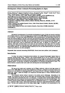
Figure 5. Annual maximum streamflow frequency plot (HEC-SSP) for Wangchhu river 3.4 Rating Curve Based on the available water level and streamflow data rating curve for the three rivers – Lungtengphung on Thimpu, Tamchhu on Wangchhu, and Haa on Haa Chu River were established (Figure 6).
78
www.ccsenet.org/jgg
Journal of Geography and Geology
Vol. 7, No. 2; 2015
Rating Curve: Lungtengphung on Thimpu 5.0
Q = 27.131(h)1.2596 R² = 0.8767
4.5
Stage (h), m
4.0 3.5 3.0 2.5 2.0 1.5 1.0 0.5 0.0 0
100
200
300 400 Discharge (Q), cumecs
500
600
700
60
70
Rating Curve: Haa on Haa Chhu 3.0
Q= 6.8559(h)1.6221 R² = 0.7384
Stage (h), m
2.5 2.0 1.5 1.0 0.5 0.0 0
10
5.0
20
30 40 Flow (Q), cumecs
50
Rating Curve: Tamchhu on Wangchhu
4.5
Stage (h), m
4.0 3.5 Q =3.8151(h)3.1385 R² = 0.8777
3.0 2.5 2.0 1.5 1.0 0
100
200
300
400 500 600 Flow (Q), cumecs
700
800
900
Figure 6. Rating curve at Lungtengphung on Thimpu, Haa on Haa Chu and Tamchhu on Wangchhu 79
1000
www.ccsenet.org/jgg
Journal of Geography and Geology
Vol. 7, No. 2; 2015
4. Results and Discussion The result of streamflow frequency analysis (Peak Q, m3/s) (Log Pearson Type 3) for annual maximum streamflow from 1992-2007 were calculated. Model calibration and validation are two important steps in flood forecasting model application. The calibration results (01Jan2003 to 31Dec2004) are presented in Table 10, for case 1 and case 2. Table 10. Calibration result comparison
Location U/S
D/S
Sub basin A B D E C
Calibration 2003 – 2004 Case 1: Observed Data Case2: After TRMM and Observed Data NC R2 PVE NC R2 PVE 0.55 0.68 6.68 0.67 0.69 -7.60 0.67 0.84 12.32 0.82 0.84 -13.05 0.48 0.77 26.13 0.73 0.80 10.45 0.05 0.73 17.00 0.54 0.73 -3.10 0.57 0.79 19.18 0.71 0.79 9.20
Case 2 shows the good calibration; hence further validation is carried out for the case 2 model. A graphical presentation of the calibrated model, a hydrograph for each sub-basin, is presented in Figure 7.
Flow, cumecs
Flow at Paro River 180 160 140 120 100 80 60 40 20 0
Obs Flow
Outflow, Computed
Date
Flow at Thimpu River 120
Obs Flow
Flow, cumecs
100 80 60 40 20 0
Date
80
Outflow, Computed
www.ccsenet.org/jgg
Journal of Geography and Geology
Vol. 7, No. 2; 2015
Flow at Wangchhu River, (Tamchhu) 320
Obs Flow
Outflow, Computed
Flow, cumecs
280 240 200 160 120 80 40 0
Date
Flow at Haa River
Flow, cumecs
40
Obs Flow
Outflow, Computed
30 20 10 0
Date
Flow at Chimakoti Dam on Wan, Outlet 700
Flow, cumecs
600
Obs Flow
Outflow, Computed
500 400 300 200 100 0
Date Figure 7. Observed and calibrated hydrograph for all stations 81
www.ccsenet.org/jgg
Journal of Geography and Geology
Vol. 7, No. 2; 2015
Model Validation The model was validated using a time series rain and flow data from 01Jan2005 to 31Dec2005. The validated results are tabulated in Table 11. Table 11. Validation result Location U/S
D/S
Sub basin A B D E C
Validation 2005 NC R2 PVE 0.52 0.67 -16.98 0.83 0.90 -21.04 0.53 0.80 13.75 0.12 0.77 -2.08 0.58 0.86 15.75
From the validated result it can be seen that NC is 83% at sub-basin B, while at sub-basin E it is 12%. Low NC at sub-basin E shows poor performance of the model, and the reasons may be: i) ungauged area, lack of data availability, or ii) validation time span. But the coefficient of determination noted at sub-basin E is 0.77. The downstream sub-basin NC is 0.58 and R2 0.86, hence the calibrated model can be used for flood forecasting application as well a warning system.
Figure 8. Comparison of flow at outlet Chimakoti Dam on Wan 4.1 Discussion The model shows poor efficiency without upstream rainfall gauges. The model run using calibrated parameters and TRMM rain data (Figure 8) showed that in case the observed data is not available, the TRMM rain data may be used to forecast floods. The percent volume error is lower than that of the actual calibrated model. The percent volume error downstream is -7.03%. There is only a major difference in the Paro and Haa Rivers at sub-basin A and E respectively in terms of the Nash–Sutcliffe model efficiency coefficient (NC), which is less than 0.50. At the outlet/downstream part of the basin, R2, NC > 0.50. The model did not incorporate the snowmelt condition due to lack of data. The sediment transport is also not incorporated in the model. Some rain gauge data is missing for 2009-2010 (Dochula) and other stations, which may create a problem in real time forecasting and accuracy. The model has been calibrated for 2003-2004 and validated for 2005, 2009 and 2010 data. A new station Begana has been added in the model. This model can be replicated for other basins. The WRF result for Bhutan is poor, thus other sources of rainfall prediction need to be incorporated in the model. An accurate rainfall forecast is essential to produce flood forecasts for mountainous river basins in Bhutan. The model did not consider snowmelt and sediment transport due to lack of data. The observed hydro-met data, gathered on an hourly basis, is crucial for Bhutan so that the model can run 82
www.ccsenet.org/jgg
Journal of Geography and Geology
Vol. 7, No. 2; 2015
in 3- to 6-hour intervals. For example, Dochula station should be replaced immediately to improve accuracy. Acknowledgement This research funded by Danida under the Danida Climate and Development Action Programme. The Hydro Met Services Division under the Department of Energy implemented in collaboration with ADPC and RIMES under the project “Support to Enhancing Adaptive Capacity to Climate Change”. The Author was the Senior Technical Specialist for ADPC and Team Leader for RIMES. References Asian Development Bank (ADB). (2014). Inception Report, Adapting to Climate Change through. IWRM. Contract N° CDTA BHU-8623. Bawa, K., & Kadur, S. (2012). Himalaya: Mountains of Life, Felis Creations Pvt Ltd. Bolch, T., Buchroithner, M. F., Peters, J., Baessler, M., & Bajracharya, S. (2008). Identification of glacier motion and potentially dangerous glacial lakes in the Mt. Everest region/Nepal using spaceborne imagery. Natural Hazards and Earth System Sciences, 8, 1329-1340. Bookhagen, B., & Burbank, D. W. (2010). Toward a complete Himalayan hydrological budget: Spatiotemporal distribution of snowmelt and rainfall and their impact on river discharge. J. Geophys. Res., 115(F3), F03019. http://dx.doi.org/10.1029/2009JF001426 Clague, J. J., & O'Connor, J. E. (2015). Chapter 14-Glacier-Related Outburst Floods. Snow and Ice-Related Hazards, Risks and Disasters. J. F. S. H. Whiteman. Boston, Academic Press: 487-519. Dey, D. (2002). Watershed Conservation And Management Of Glacial Lake Outburst Flood; Combating Climate Change In Himalayan Environment, South Asian Forum for Environment, Calcutta, India. Elalem, S., & Pal, I. (2014). Mapping the vulnerability hotspots over Hindu-Kush Himalaya region to flooding disasters. Weather and Climate Extremes. http://dx.doi.org/10.1016/j.wace.2014.12.001 FAO/IIASA/ISRIC/ISSCAS/JRC. (2009). Harmonized World Soil Database (version 1.1), FAO, Rome, Italy and IIASA, Laxenburg, Austria. Fujita, K., Nishimura, K., Komori, J., Iwata, S., Ukita, J., Tadono, T., & Koike, T. (2012). Outline of Research Project on Glacial Lake Outburst Floods in the Bhutan Himalayas. Global Environmental Research, 16, 3-12. Griffis, V., & Stedinger, J. (2007). Evolution of Flood Frequency Analysis with Bulletin 17. Journal of Hydrologic Engineering, 12(3), 283-297. http://dx.doi.org/10.1061/(ASCE)1084-0699(2001)6:4(293) Griffis, V., & Stedinger, J. (2008). Flood Frequency Analysis in the United States: Time to Update. Journal of Hydrologic Engineering, 199-204. http://dx.doi.org/10.1061/(ASCE)1084-0699(2008)13:4(199) IPCC. (2013). Managing the Risks of Extreme Events and Disasters to Advance Climate Change Adaptation. In V. B. C. B., T. F. Stocker, D. Qin, D. J. Dokken, K. L. Ebi, M. D. Mastrandrea, K. J. Mach, G. K. Plattner, S. K. Allen, M. Tignor, & P. M. Midgley (Ed.), A Special Report of Working Groups I and II of the Intergovernmental Panel on Climate Change (pp. 582). Cambridge, UK, and New York, NY, USA. Hansen, M. C., Defries, R. S., Townshend, J. R. G., & Sohlberg, R. (2000). Global land cover classification at 1 km spatial resolution using a classification tree approach. International Journal of Remote Sensing, 21(6), 1331 - 1364. http://dx.doi.org/10.1080/014311600210209 Liu, J. S., Wang, Zh. Y., Gong, T. L., & Uygen, T. (2012). Comparative analysis of hydroclimatic changes in glacier-fed rivers in the Tibet- and Bhutan-Himalayas. Quaternary International, 282(19), 104-112. http://dx.doi.org/10.1016/j.quaint.2012.06.008 Mool, P. K., Wanda, D., Bajracharya, S. R., Kunzang, K., & Joshi, S. P. (2001). Inventory of Glaciers, Glacial Lakes and Glacial Lake Outburst Floods. Monitoring and Early Warning Systems in the Hindu Kush-Himalayan Region Bhutan. ICIMOD and UNDP- ERA-AP. NEC. National Environment Commission. (2014). Draft Water regulations. SDMC. (2010). South Asia Disaster Report 2010. SAARC Disaster Management Centre, New Delhi. South Asian Flood (SAF). (2014). country_code=BH&c_id=7
Retrieved
from
http://southasianfloods.icimod.org/contents.php?
Watershed Management Department (WMD). MOAF, RGOB. (2011). A roadmap for watershed management in 83
www.ccsenet.org/jgg
Journal of Geography and Geology
Vol. 7, No. 2; 2015
Bhutan. Wang, X., Liu, S. Y., Guo, W. Q., & Xu, J. (2008). Assessment and simulation of glacier lake outburst floods for Longbasaba and Pida Lakes, China. Mountain Research and Development, 28, 310-317. http://dx.doi.org/10.1659/MRD-JOURNAL-D-09-00042.1 Westoby, M. J., et al. (2014). Modelling outburst floods from moraine-dammed glacial lakes. Earth-Science Reviews, 134(0), 137-159. http://dx.doi.org/10.1016/j.earscirev.2014.03.009 Xue, X., Hong, Y., Limaye, A. S., Gourley, J., Huffman, G. J., Khan, S. I., … Chen, S. (2013). Statistical and Hydrological Evaluation of TRMM-based Multi-satellite Precipitation Analysis over the Wangchu Basin of Bhutan: Are the Latest Satellite Precipitation Products 3B42V7 Ready for Use in Ungauged Basins? Journal of Hydrology, 499(30), 91-99. http://dx.doi.org/10.1016/j.jhydrol.2013.06.042 Copyrights Copyright for this article is retained by the author(s), with first publication rights granted to the journal. This is an open-access article distributed under the terms and conditions of the Creative Commons Attribution license (http://creativecommons.org/licenses/by/3.0/).
84