Development of New Probability Model with Application in ... - iMedpub

Available online at www.pelagiaresearchlibrary.com Pelagia Research Library Advances in Applied Science Research, 2011, 2 (4):306-313

ISSN: 0976-8610 CODEN (USA): AASRFC

Development of New Probability Model with Application in Drinking Water Quality Data Kishore K. Das1, Bhanita Das*1, Bhupen K. Baruah,2 and Abani K. Misra2 1

Department of Statistics, Gauhati University, Assam, India Department of Chemistry, Gauhati University, Assam, India _____________________________________________________________________________ 2

ABSTRACT In this paper, we develop length biased distribution (LBD) of weighted Inverse Gaussian distribution (WIGD). Moment properties, estimation of parameter, and hazard function of the resulting distribution have been considered here. Finally, we illustrate the applicability of LBD of WIGD in environmental sciences using drinking water quality data based on Fluoride (F) concentration respectively. Keywords: Weighted Inverse Gaussian distribution (WIGD), Length biased distribution (LBD), Drinking water quality. _____________________________________________________________________________ INTRODUCTION Water quality performs important role in health of human, animals and plants. The quality of water within a region is governed by both natural processes such as rainfall, the underlying geology, weathering processes, the vegetation or organic matter decay, soil erosion and anthropogenic effects viz. urban, industrial and agricultural activities and the human exploitation of water resources [12]. In the current world economic paradigms, sustainable socioeconomic development of every community depends much on the sustainability of the available water resources. Water of adequate quantity and quality is required to meet growing household, industrial and agricultural needs. Groundwater quality is a very sensitive issue, which transcends national boundaries. Therefore, quality of water resources is a subject of ongoing concern and the assessment of long term water quality changes is also a challenging problem. During the last decades, there has been an increasing demand for monitoring water quality by regular measurements of various water quality parameters. According to [13], some of the necessities of water quality monitoring are- to provide a system wide synopsis of water quality, to monitor long-range trends in selected water quality parameters, to detect actual or potential water quality 306 Pelagia Research Library

Bhanita Das et al Adv. Appl. Sci. Res., 2011, 2 (4):306-313 _____________________________________________________________________________ problems, to determine specific causes, to assess the effect of any convective action and to enforce standards. Therefore, the effective, long-term management of ground water requires a fundamental understanding of hydro-morphological, chemical and biological characteristics. However, due to spatial and temporal variations in water quality (which are often difficult to interpret), a monitoring program, providing a representative and reliable estimation of the quality of ground waters is necessary [2]. Computer systems now offer the possibility of handling and manipulating very large databases in ways which were not previously a practical option. [14] have used such databases for estimation of mass loads of pollutants in rivers. [15] used the hydrochemical databases from upland catchments for a period of five years to assess the annual variation in amounts and concentration of solutes and to examine the variation in stream water quality due to changes in flow, season and long time trend. A variety of statistical methods such as cluster analysis (CA), principal component analysis (PCA) and factor analysis (FA) have been exerted for a variety of environmental applications, containing evaluation of ground water monitoring sources and hydrographs, examination of spatial and temporal patterns of water quality, identification of chemical species related to hydrological conditions and assessment of environmental quality indicators [16], [18], [29]. These methods display the information which is concealed in the quality variables observed in a water quality monitoring network. Application of these multivariate statistical techniques, helps in the interpretation and representation of complex data matrices to better understand the water quality and ecological status of the studied systems, enabled the classification of water samples into distinct groups on the basis of their hydrochemical characteristics, allows the identification of possible factors sources that influence water systems and offers a valuable tool for reliable management of water resources, as well as rapid solution to pollution problems [11], [21], [23], [24], [28], [30]. Distribution model study is one of the recent developments in statistical analysis of environmental research. Development of new distributions definitely helps to interpret the spatial and temporal variation of hydro-morphological as well as physico-chemical quality of ground water easily and concerted strategies can be adopted for better future. Distribution study can successfully be used to be derived information from the data set about the possible influences of the environment on water quality and also identify natural groupings in the set of data. These methods are important to avoid misinterpretation of environmental monitoring data due to uncertainties. Water quality data do not usually follow convenient probability distributions such as the well-known normal and lognormal distributions on which many classical statistical methods are based [9]. Probability plots are used to determine how well data fit a theoretical distribution. This could be achieved by comparing curves of measured values to the density curve of theoretical distributions. The concepts of length-biased (LB) and weighted distributions (WD) have been applied in various fields such as ecology and environmental sciences for reliability and survival analysis [3]. The LB and WD distributions occur naturally in many situations because sometimes it is not possible to work with a truly random sample from the population of interest. [17] mentioned that in environmental studies, observations fall in the non-experimental, non- replicated and non307 Pelagia Research Library

Bhanita Das et al Adv. Appl. Sci. Res., 2011, 2 (4):306-313 _____________________________________________________________________________ random categories. Therefore, making random selection from the observed population is impossible. Thus, problems of model specification and data interpretation acquire great importance. A way of confronting this problem is by considering observations which are selected with probability proportional to their ‘length’. The resulting distribution is called the lengthbiased distribution. On the other hand, non-observation and damage of dataset results reduction of value or adoption of a sampling plan which gives unequal probabilities to the various units and cannot be considered as a random sample from the theoretical distribution [20]. For these types of data sets the weighted distribution can be applied. Both these distributions takes into account the method of ascertainment by adjusting the probabilities of actual occurrence of events to arrive at a specification of the probabilities of those events as observed and recorded [10]. In this paper, LBD of WIGD have been developed and an attempt has been made to apply these newly developed distribution to the estimated data of fluoride(F) during the study that can be useful in environmental field in near future to provide a comprehensive description of the statistical and probabilistic properties. Preliminary computation of estimated data of fluoride (F) during the study showed that the observed frequencies of these data were well fitted with the shape of the theoretical LBD of WIGD. Therefore, in this paper, LBD of WIGD has been considered to illustrate the applicability of the new probability distribution model. MATERIALS AND METHODS Sampling was done using a stratified simple random procedure from 1st March to 31st October, 2009 in three administrative sub-divisions of Nagaon district of Assam, India by B.K. Baruah and A.K. Mishra. A total of 78 water samples (66 Tube Well, 8 Deep Tube Well, 2 Ring Well and 2 Supply Water) were collected randomly from 9 villages from three sub-divisions viz. Nagaon, Kaliabor, and Hojai. Three villages from Hojai sub-division viz. Nilbagan, Udali and Dimoru, five stations from Nagaon sub-division (Kampur Town, South Haibargaon, Halowabhakatgaon, Baruabli and Barghat) and greater Kaliabor town area were selected randomly for water sampling which is in 5 km minimum distance apart. Out of the total bore well or ring well water sources 74% sources are only source of water and 26% sources are complementary source of water. Water samples were collected after 10 minutes of initial pumping in pre-cleaned polythene containers of one liter capacity, were rinsed out 3-4 times and transported to laboratory at 100C. The containers were filled up to the mouths and then tightly stopper to avoid contact with air or to prevent agitation during transport. The storage and preservation of samples were done with standard procedure [1]. Water temperature and pH are measured at the time of collection of the sample. In the laboratory water samples were vacuum filtered using 0.45 µm pre-washed and pre-weighed membranes and the filtrates containing dissolved metals were poured in to clean plastic containers then acidified with concentrated nitric acid to pH 2 to 3. The water quality parameter estimation and calibration of equipments were done using standard methods and techniques [1] and [27]. 308 Pelagia Research Library

Bhanita Das et al Adv. Appl. Sci. Res., 2011, 2 (4):306-313 _____________________________________________________________________________ The presence of fluoride in ground water is attributed to the geological deposits, geochemistry of the location, waste disposal and application of chemical fertilizers and pesticides. Fluoride the most electronegative element taking thirteenth position in order of abundance constituting about 0.077 of the earth crust is widely distributed in both igneous and sedimentary rocks principally as fluorspar cryolite and fluorapatite where from finds its pathway to ground water systems [6]. The water bodies may also be contaminated by fluorides from domestic sewage and agricultural runoff if phosphate fertilizers manufactured from phosphate rocks containing fluorapatites are applied domestic sewage and irrigation with water containing small amount of fluoride ions would tend to concentrate these ions in soil water [8]. High concentration of fluoride in water causes dental skeletal and non-skeletal fluorosis. The Ca2+ concentration in bones and teeth are relatively high and fluoride gets deposited on these as calcium fluorapatite [26]. In dental fluorosis yellow patches are formed on teeth for fluoride deposition, which eventually turns black. Due to this the teeth may be pitted perforated and chipped off at the final stage. In skeletal fluorosis fluoride deposition occurs in bones and results severe pain in back bone joints pelvic column etc. In addition to dental and skeletal fluorosis excessive fluoride in drinking water may cause several ailments viz. neurological manifestations muscular manifestations allergic manifestations urinary tract manifestations gastrointestinal manifestations etc. These are collectively termed as non-skeletal fluorosis. Fluoride is also known to induce aging [8]. For children of below 8 years of age fluoride is beneficial when present in concentration of 0.81.0mg/L for calcification of dental enamel [6]. The fluoride concentration is found higher than the permissible limit of 1.5 ppm in 39.1% water samples and prevalence of dental fluorosis was found in the variation from as low as 0.27% to 18.7%. Weighted distribution To introduced the concept of a weighted distribution, suppose X is a non negative random variable with probability density function (pdf) f X ( x ) and the weighted version of ‘x’ with weight function w(x) which we can denote by the random variable (r.v.) X w and whose distribution is called the weighted distribution, has pdf given by [20] w( x ) f X ( x ) ;x > 0 E [w( x )] Assuming that E [w( x )]< ∝ i.e. the first moment of w(x) exists. Where, mean µ = E [x ] . f X w (x ) =

Length biased distribution Similarly, the length biased distribution is a particular case of weighted distribution which can be denoted by random variable (r.v.) ‘t’ which has probability density function (pdf) expressed as t f X (t ) f T (t ) = ; t > 0 ; µ > 0 , where µ = E [x ]

µ

Weighted Inverse Gaussian Distribution (WIGD) The standard form of the two-parameter inverse Gaussian distribution is given by [5] 1

 λ x µ   λ 2  − 2 +  , x > 0, µ, λ > 0 PX (x; µ, λ) =  exp − 3 x   2πx   2µ  µ

(1)

309 Pelagia Research Library

Bhanita Das et al Adv. Appl. Sci. Res., 2011, 2 (4):306-313 _____________________________________________________________________________ λ  We use the weight function w(x) = x 2 exp  , x > 0, λ > 0 in the two parameter Inverse  2x  Gaussian distribution having pdf (1), then the WIGD is obtained as 3

 λ 2 1  2  2µ  2 f X (x ) =  x exp − λx / 2µ 2 , x > 0, µ, λ > 0 w 3 Γ( ) 2

(

)

( 2)

Length Biased distribution of WIGD If X is a non negative r.v. with pdf f ( x ) then using (2) the Length biased distribution of weighted inverse Gaussian distribution (LBD of WIGD) is given as 5 3  λx  λ2 f L (x ) = x 2 exp − 2 ; x > 0, µ, λ > 0 (3) 3  2µ  3 3µ 5 2 2 Γ   2 Properties of LBD of WIGD The rth order raw moment for LBWIGD is given as 5  2 r µ 2r Γ  r +  2  EX r = r L 3λ The moment generating function of LBWIGD is given as −5  2µ 2 t  2 M X (t ) = 1 −  L λ   The cumulant generating function of the LBD of WIGD is given as 5  2µ 2 t   K X (t ) = − log1 − L 2  λ  The characteristic function of LBD of WIGD is given as 5 −  2µ 2 it  2 Φ X (t ) = 1 −  Li λ   The first four moments and cumulants are as follows 5µ 2 10 µ 4 40 µ 6 540 µ 8 κ 1 = µ1′ = ,κ 2 = µ 2 = 2 ,κ 3 = µ3 = 3 ,κ 4 = µ 4 + 3κ 2 = 2 λ λ λ λ4 The recurrence relation for moments is given as 2µ 2  5 µ ′= r + µ ′  r +1 λ  2 r The cumulative distribution function (cdf) of LBWIGD is given as

[ ]

310 Pelagia Research Library

Bhanita Das et al Adv. Appl. Sci. Res., 2011, 2 (4):306-313 _____________________________________________________________________________

FX

(x ) =

5 λ2

 λ − 2 ∞   2µ ∑ j! j =0

  

j

5 x 2 5   j+  2  j+

3 3 3µ 5 2 2 Γ   2 The hazard function of the LBWIGD is given by 5 5  λx  λ2 x 2 exp − 2  3  2µ  3 5 2 3µ 2 Γ   2 hX ( f ) = , x > 0, µ, λ > 0 j L 5  λ  5   −   + j 2  ∞  2  2 µ λ2 x   1− ∑ 3 j ! 5  j =0 + j  3   2  3µ 5 2 2 Γ   2   Estimation Using the method of moments the estimation of the parameter for LBD of WIGD are given by 5µ 2 , where m ′ the sample moment and the value of is µ is assumed as data mean. λ= 1 m′ L

1

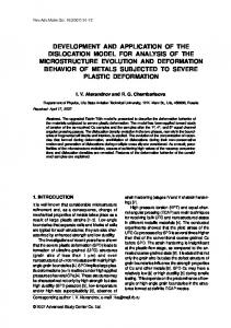
Application The chi-square test of goodness of fit is applied to drinking water quality data. The no. of class intervals over which the computations were found was 5 for Fluoride concentration. Fitting of LBD of WIGD (F) was performed by Simpson’s Rule of numerical integration with the help of C++. Table 1: Fitting of LBD of WIGD for Fluoride Concentration (F) in water quality. Class Interval 1.33 λ = 4.25, µ = 0.78, χ 2 = 2

Observed Frequency(Oi)

Expected Frequency(Ei)

6 18 15 12 8

6 15 14 12 12

(Oi − Ei )2

Ei

0 0.6 0.07 0 1.33

311 Pelagia Research Library

Bhanita Das et al Adv. Appl. Sci. Res., 2011, 2 (4):306-313 _____________________________________________________________________________ Graphical Representation of WIGD

CONCLUSION In this article, the LBD of WIGD was developed. This new distribution is turns out to be quite flexible for modeling water quality. An application to the real data showed that this new model is a flexible alternative to other well known models. Thus, we have developed a new probability models which might be of use for practitioners in the environmental sciences. Here we postulated that LBD of WIGD is appropriate for modeling water quality. REFERENCES [1] APHA; Standard methods for the examination of water and wastewater, New York: APHA. AWWA and WEF, 1995 (20th Ed.). [2] Dixon, W., Chi swell B., Water Res., 1996, 30 (9), 1935-1948. [3] Gupta R.C., Kirmani S. Comm. Stat Theory Meth, 1990, 19:3147-3162. [4] Ibrahim, K., Kamil, A. A., and Mustafa, A., Advances in Applied Science Research., 2010, 1(1); 1-8. [5] Johnson N. L., Kotz S., Balakrishnan N., Continuous univariate distributions. 1995, vol. 2. Wiley, New York. [6] Kannan K., Fundamentals of Environmental Pollution. 1991, S. Chand and Company Ltd. New Delhi. India. 312 Pelagia Research Library

Bhanita Das et al Adv. Appl. Sci. Res., 2011, 2 (4):306-313 _____________________________________________________________________________ [7] Khadar Babu, S. K., Karthikeyen, K., Ramanaiah, M. V., and Ramanah, D., Advances in Applied Science Research., 2011, 2(2); 128-133. [8] Kumar S. and D. K. Saini., Journal of Environment and Pollution; 1998, 5(4) p. 299-305. [9] Lee, J. Y., Cheon J. Y., Lee K. K., Lee S. Y., Lee M. H., J. Environ. Qual., 2001, 30, 15481563. [10] Leiva V., Baros M., Paula G. A., Sanhueza A., Environmetrics, 2008, 19, doi; 10.1002/env. 861(in press). [11] Lettenmaier R. P., Hooper E. R., Wagoner C., and Fans, K. B., Water Resource. Res., 1991, 27, 327–339. [12] Liao, S. W., Gau, H. S., Lai, W. L., Chen J. J., Lee C. G., J. Environ. Manag. 2007, 88 (2), 286-292. [13] Liebetrau A.M., Water Resource. Res., 1979, 15, 1717–1728. [14] Littlewood, I.G., Watts, C.D. and Custance, J.M., Sci. Total Envir., 1998, 210, 21–40. [15] Miller J.D. and Hirst, D., Sci. Total Envir., 1998, 216, 77–88. [16] Ouyang, Y., Water Res., 2005, 39 (12), 2621-2635. [17] Patil G. P., Weighted distributions, Encyclopedia of environmetrics, 2002, vol 4. Wiley, Chichester , pp. 2369-2377 [18] Perkins, R. G., Underwood, G. J. C., Gradients of chlorophyll a and water chemistry along an eutrophic reservoir with determination of the limiting nutrient by in situ nutrient addition, Water Res., 2000, 34 (3), 713-724. [19] Ramanah, D. V., Ramanaiah, M. V., Khadar Babu, S. K., Karthikeyen, K., Advances in Applied Science Research., 2011, 2(2); 284-289 [20] Rao. C.R., Weighted distributions arising out of methods of ascertainment: What population does a sample represent, Celebration of Statistics, 1985 [21] Reghunath R., Murthy T. R. S., Raghavan, B. R., Water Res., 2002, 36 (10), 2437-2442. [22] Sharma, J. R., Guha, R. K. and Sharma, R., Advances in Applied Science Research., 2011, 2(1); 240-247. [23] Singh K. P., Malik A., Mohan D., Sinha S., Water Res., 2004, 38 (18), 3980-3992. [24] Singh K. P., Malik A., Sinha S., Analytical Chimica. Acta., 2005, 538 (1-2), 355-374. [25] Singh, S. and Shah, R. R., Advances in Applied Science Research., 2010, 1(1); 66-73. [26] Suresh, I. V., A. Wanganeo, C. Padmakar, and R. G. Sujatha, Ecology Environment and Conservation; 1996, 2(1-2), 11-15. [27] Trivedy, R. K., Goel P. K., and Trisal C.C., Practical Methods in Ecology and Environmental Sciences, 1987, Environmental Publication, Karad, India. [28] Vega, M., Pardo R., Barrado E., Deban L., Water Res., 1998, 32 (12), 3581-3592. [29] Voutsa, D., Manoli, E., Samara, C., Sofoniou, M., Stratis I., Water Air Soil Pollut., 2001, 129 (1-4), 13-32. [30] Wunderlin, D. A., Diaz, M. P., Ame, M. V., Pesce, S. F.; Hued, A. C.; Bistoni, M. A., Water Res., 2001, 35 (12), 2881-2894 .

313 Pelagia Research Library