DEVELOPMENT AND APPLICATION OF A BIOENERGETICS. MODEL FOR GIZZARD SHAD by. SCOTT H. SEBRING, B.A.. A THESIS. IN. FISHERIES SCIENCE.
DEVELOPMENT AND APPLICATION OF A BIOENERGETICS MODEL FOR GIZZARD SHAD by SCOTT H. SEBRING, B.A. A THESIS IN FISHERIES SCIENCE Submitted to the Graduate Faculty of Texas Tech University in Partial Fulfillment of the Requirements for the Degree of MASTER OF SCIENCE
Approved
Dean of the Graduate School December, 2002
ACKNOWLEDGEMENTS
I would like to thank Drs. Gene R. Wilde, Reynaldo Patiiio, Richard E. Strauss, Kevin L. Pope, and Loren M. Smith for the support and direction they provided while serving on my thesis committee. I also thank Dr. David Wester for his comments and help in developing the Monte Carlo and correlation analysis procedures used for error analysis. I thank Drs. Lars Rudstam, Donald Stewart, and Kyle Hartman for their assistance answering a multitude of questions pertaining to bioenergetics modeling. I thank the numerous people who helped with laboratory experiments, collecting fish in the field, and were exceptional friends and colleagues: Monte Brown, Chris Chizinski, Bart Durham, Kevin Offill, Jesse Shuck, Matt Gray, Jessica Emrich, and Tracie Stuart. I thank Jerry Robison and the Village of Buffalo Springs Lake for allowing me access to the lake to collect fish. I thank the many people who provided daily temperature and growth data for gizzard shad: Jeff Boxrucker and the Oklahoma Department of WildUfe Conservation; Donna Cobb and Bill Matthews of the University of Oklahoma Lake Texoma Biological Station; Paul Michaletz and the Missouri Department of Conservation; and Bill Thompson and the Florida Fish and Game Commission. Finally, I would like to thank Terry, Laurie, Marc, Lindsey, Carl J. Ronning, and Sagrario Mejia, for without their love and support during my research and educational experience at Texas Tech University I would not have become the biologist and the person I am today.
11
TABLE OF CONTENTS
ACKNOWLEDGMENTS
ii
LIST OF TABLES
iv
ABSTRACT
v
LIST OF FIGURES
Vi
CHAPTER L INTRODUCTION
1
n. METHODS
9
m . RESULTS
28
IV. DISCUSSION
54
V. CONCLUSIONS
61
REFERENCES
62
APPENDDC A. SAS PROGRAM USED FOR ERROR ANALYSIS WHEN PARAMETER VARIANCES ARE 2% OF NOMINAL VALUE
72
B. SAS PROGRAM USED FOR ERROR ANALYSIS WHEN PARAMETER VARIANCES ARE 10% OF NOMINAL VALUE
76
C. SAS PROGRAM USED FOR ERROR ANALYSIS WHEN PARAMETER VARIANCES ARE 20% OF NOMINAL VALUE
80
111
ABSTRACT
I developed a bioenergetics model for gizzard shad using a combination of laboratory and literature derived parameter estimates. I estimated allometric intercepts and slopes for consumption (CA = 0.8081, CB = -0.30) and respiration (RA = 0.005, RB -0.21) and optimum and maximum temperatures for consumption (CTO = 25°C, CTM = 32.4°C) and respiration (RTO = 32.4°C, RTM= 35.4°C). I used the model to simulate growth of gizzard shad in sbc lakes with literature derived diet and site-specific temperature and size- at-age data to estimate values of;? that were similar to those of other fishes. The model for gizzard shad is applicable for use in lakes, reservoirs, and sfreams that vary in productivity, substrate, and size. In general, growth of gizzard shad m southern lakes changed more than in northern lakes when diet composition, water terrqjerature, and activity were modified. Modifying diet composition, water temperature, and activity change growth of gizzard shad more in southern lakes than in northern lakes because temperatures in lakes such as Lake Apopka, Florida, are near the upper thermal limit of gizzard shad.
IV
LIST OF TABLES
1. The optimum temperature of respiration (RTO) of 35.4°C was estimated by heating gizzard shad at an average rate of 0.3°C x minute"'
36
2. Bioenergetics model parameter estimates for consumption, respiration, excretion, and egestion
40
3. Growth of gizzard shad was simulated in three separate sets with bioenergetics model parameters having variances of 2%, 10%, or 20% at water temperatures of 5, 10, 15, 20,25, 30, and 32°C. Parameters were ranked from greatest to least affect on growth using Pearson correlation (PS) and max-R regression (MR)
42
4. Percent change in simulated growth of gizzard shad when diet composition is 75% zooplankton, 75% phytoplankton, or 75% detritus
51
5. Percent change in simulated growth from baseline when water temperature is increased by 3.3°C for age-1, age-2, age-3, and age-4 gizzard shad
52
6. Percent change in baseline growth when activity is modified to 1, 2, 3, or 4 for age-1, age-2, age-3, and age-4 gizzard shad
53
LIST OF FIGURES
1. Daily surface temperature in Acton Lake, Ohio, in 1974 was predicted using a multinomial regression equation from Pierce (1977)
22
2. Daily water temperature in Lake Apopka, Florida, 1997 (from Bill Johnson, Florida Fish and Game Commission, 2001). Water temperatures in late November through February were assumed to be less than observed water temperatures
23
3. Average monthly water temperatures in Lake Erie, Ohio from 1980 to 1993 were used to create a polynomial regression equation and estimate daily water temperatures and winter temperatures were assumed when not available. In the regression equation X is the day of year, 1 to 365
24
4. Daily and bi-monthly observed surface water temperature in Pomme De Terre Lake, Missouri in 1988 (from Paul Michaletz, Missouri Department of Conservation, 1997)
25
5. Daily and bi-monthly surface water temperature in Stockton Lake, Missouri in 1988 (from Paul Michaletz, Missouri Department of Conservation, 1997)
26
6. Daily surface temperatures in Lake Texoma, Oklahoma-Texas in 1994 (from Donna Cobb, University of Oklahoma Biological Station, 2002)
27
7. Specific respfration (g oxygen g fish'' day'') by gizzard shad at 10, 15, 20, 25, and30°C
34
8. Average specific respiration (g oxygen g fish'' day') by gizzard shad was obtained from Pierce (1977) and used to estimate RA using non-linear regression. The allometric equation for respiration is a function of mass, W, measured near the i?rO at the standard metabolic rate
35
9. Average specific consumption (prey x g predator'' x day') by gizzard shad at 10, 15, 20, and 25°C were used to estimate e g
37
10. Specific consumption by gizzard shad at CTO was used to estimate the allometric parameters for consumption, CA and CB using non-linear regression. Allometric parameters for CA and CB were different when excluding (A) and including (B) an 84 gram fish in the analysis
38
VI
11. Natural log of average specific consumption and temperatures < CTO were used to estimate the temperature-dependent slope for consumption, CQ
39
12. Sensitivit> anal\scs of the gizzard shad bioenergetics parameters for one year of simulated growth in Lake Eric. The absolute values of sensitivity indices for all parameters are listed when parameter estimates are increased and decreased by 10% of their nominal values
41
13. Baseline simulated growth of ago-1 gizzard shad in six lakes in the eastern and central United States (A; Acton, Apopka, and Erie, B; Pomme De Terre, Stockton, and Texoma)
43
14. Baseline simulated growth of age-2 gizzard shad in six lakes in the eastern and central United States (A; Acton, Apopka, and Erie, B; Pomme De Terre, Stockton, and Texoma)
44
15. Baseline simulated growth of age-3 gizzard shad in Lake Apopka, Pomme De Terre Lake, Stockton Lake, and Lake Texoma
45
16. Baseline simulated growth of age-4 gizzard shad in Pomme De Terre Lake, Stockton Lake, and Lake Texoma
46
17. Baseline simulated specific growth rates of age-1 gizzard shad in six lakes in the eastern and central United States (A; Acton, Apopka, and Erie, B; Pomme De Terre, Stockton, and Texoma)
47
18. Baseline simulated specific growth rates of age-2 gizzard shad in six lakes in the eastern and central United States (A; Acton, Apopka, and Erie, B; Pomme De Terre, Stockton, and Texoma)
48
19. Baseline simulated specific growth rates of age-3 gizzard shad in Lake Apopka, Pomme De Terre Lake, Stockton Lake, and Lake Texoma
49
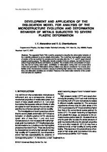
20. Baseline simulated specific growth rates of age-4 gizzard shad in Pomme De Terre Lake, Stockton Lake, and Lake Texoma
50
vii
CHAPTER I INTRODUCTION Gizzard shad (Dorosoma cepedianum) are distributed from the Rio Panuc6 River of northeastern Mexico to southeastern Canada and are the most common prey fish in aquatic ecosystems of the eastern United States (Noble 1981). They are consumed by as many as 17 fishes (Miller 1960) and are preferred to sunfishes by largemouth bass (Lewis and Helms 1964). The diet of gizzard shad is broad and consists of aquatic insects, zooplankton, phytoplankton, and defritus (Miller 1960; Bodola 1966; Jenkins 1957; Jude 1973). Gizzard shad reach densities as great as 86 fish x m'^ (Stein and DeVries 1992) and in the absence of sufficiently abundant predators (Jenkins 1957; Dalquest and Peters 1966; Johnson et al. 1988), grow rapidly to a size that makes them invulnerable to age-0 piscivores (Megrey 1978; Pierce et al. 1981; Adams and DeAngelis 1987; Johnson et al. 1988; Lazarro et al. 1992; Stein et al. 1995; Roseman et al. 1996; Shepherd and Mills 1996), and as larvae compete with young of other fish species, which decreases growth and recruitment of predatory fishes (DeVries et al. 1991; Pope and DeVries 1994, Stein et al. 1995; 1996; Garvey and Stein 1998a; 1998b). Because gizzard shad often regulate production in lentic ecosystems and alter abundances and composition of plankton communities (Vanni 1987; Drenner et al. 1982; DeVries and Stein 1992; Turner and Mittelbach 1992; Stem et al. 1995; Dettmers and Stein 1996; Shepherd and Mills 1996; Bremigan and Stein 1997; Garvey and Stein 1998), they are important in the transfer of energy from primary producers to secondary consumers in aquatic communities (Jester and Jensen 1972; Adams and DeAngelis 1987; Johnson et al. 1988; DeVries et al. 1991;
Stein et al. 1996; Dreimer et al. 1998; Bremigan and Stein 1999). Periodic mass mortality of gizzard shad occur (Miller I960; Bodola 1966) yet, they have been introduced, or removed, from lentic systems m the United States more frequently than any other prey fish (DeVries and Stein 1990). Understanding differences in growth rates due to diet composition and activity of gizzard shad are important to managing lentic systems of the central and eastern United States. Fishery scientists must develop quantitative methods to improve management of aquatic ecosystems in order to predict growth and consumption according to regional temperature (Brandt and Hartman 1993). Bioenergetics models are potential tools that could be used to explore the effects that fish have on aquatic ecosystems (Rice and Cochran 1984). Bioenergetics models have been developed for commercially important or gamefish species, whereas relatively few models exist for prey fishes (Adams and Breck 1990; Hanson et al. 1997) such as alewife (Alosa pseudoharengus) (Stewart and Binkowski 1986), Atlantic herring (Clupea harengus) (Rudstam 1988), Atlantic menhaden (Brevoortia tyrannus) (Durbin and Durbin 1983), fathead minnow (Pimephales promelas) (Duffy 1998), and rainbow smelt (Osmerus mordax) (Lantry and Stewart 1993). However, none have been developed for gizzard shad. Bioenergetics models have been used to investigate seasonal specific-growth and consumption rates (Pierce 1977; Megrey 1978), competitive feeding interactions (Zwiefel et al. 1999), and stocking density of hybrid striped bass (Morone saxatilis x M. chrysops) necessary to regulate trophic interactions of gizzard shad in Ohio impoundments (Dettmers et al. 1998). Because they are found in a variety of habitats throughout the United States a
bioenergetics model would be ideal to investigate the effects of water temperature increase, diet composition, and activity of gizzard shad. Also, using a bioenergetics model to quantify greatest periods of growth and consumption of gizzard shad may identify sizes of gizzard shad and temperatures that are associated with trophic interactions that regulate aquatic ecosystems.
Bioenergetics Model I used the "Wisconsin" bioenergetics model (Ney 1993) for microcomputers developed by Hanson et al. (1997) to model growth and consumption by gizzard shad. Consumption and respiration parameters for this model depend on fish mass and temperature (Whitledge and Hayward 1997) and all errors become pooled in the parameter that is solved for the bioenergetics equation (Brett and Groves 1979). This model has six basic parameters:
G = C-(R + S + F+U),
(1)
where G is growth, C is consumed energy, R is the energy of respiration, S is the proportion of assimilated energy, F is the energy associated with egestion, and C/is the energy associated with excretion (Kitchell et al. 1977). Parameters for bioenergetics models can be estimated from laboratory or field studies, borrowed from closely related species, or adapted from published and unpublished literature (Hanson et al. 1997). Borrowing estimates of parameters from other fish species has been criticized because
fish may have significant life history differences (Ney 1993). However, assummg parameters from bioenergetics models of species with similar Ufe histories causes little error in model output (Hanson et al. 1997). The equation used to model consumption by warmwater fish contains three parts: an allometric function relating mass to maximum food consumption, a temperature-dependent function, and a parameter indicating the proportion of maximum consumption. The equation for consumption is:
C^C„a.r^pX/(T),
(2)
where C is the energy of consumed food, Cmax is the allometric equation for maximum specific consumption rate (g prey x g predator'' x day'),/? is the proportion of maximum consumption, and /(T) is a temperature-dependent fimction. It is important to experimentally estimate Cmax because this determines the ultimate upper bound on the growth potential offish (Kitchell 1983; Stewart and Binkowski 1986). The allometric equation for maximum consumption is obtained by examining consumption as a fimction offish mass at the optimum temperature of consumption (CTO). The first equation for the consumption parameter is an allometric equation for maximum consumption:
Cma.-^CA>^W^\
(3)
where C^ax is estimated as the product of the allometric intercept of consumption (CA), fish mass (W), and tiie allometric fimction slope of consumption (CB) (Hanson et al. 1997). The equation for consumption includes a temperature-dependent equation yfZ) for warmwater fishes. The temperature-dependent function for consumption is based on a parameter indicating the approximate increase in temperature-dependent consumption at low temperatures (CQ), the optimum temperature of consumption (CTO), and the maximum temperature for consumption (CTM). The temperature-dependent function for consumption reaches a maximum of 1 at the optimum temperature of consumption (CTO) and rapidly decreases to 0 at the maximum temperature of consumption (CTM). The second part of the consumption equation is the temperature-dependent fimction for consumption by warmwater fishes:
/rT; = CF^xe(^^''''v
\
\ •'. I
j:
•^H
1
Xi ••->
2
•^
0.000 -
11 A
o in •g cx -0.002 -
li /.'
bO
1
-0.004 -
•'•!
.
/..yfi !
f. !
•* I'
!.' A J;
1
1
May Jun
1
1
1
1
1
1
1
1
1
1
1
Jul Aug Sep Oct Nov Dec Jan Feb Mar Apr May
Figure 20. BaseUne simulated specific growth rates of age-4 gizzard shad in Pomme De Terre Lake, Stockton Lake, and Lake Texoma.
50
Table 4. Percent change in simulated growth of gizzard shad when diet composition is 75% zooplankton, 75% phytoplankton, or 75% detritus.
Lake Acton
Apopka
Erie
Pomme De Terre
Stockton
Texoma
Diet Composition zooplankton phytoplankton detritus zooplankton phytoplankton detritus zooplankton phytoplankton detritus zooplankton phytoplankton detritus zooplankton phytoplankton detritus zooplankton phytoplankton detritus
Age-1 71 24 55 67 22 55 18 8 46 68 21 57 63 20 54 80 25 61
51
Age-2 52 18 45 62 19 54 34 II 35 57 17 52 54 17 50 61 20 53
Age-3
Age-4
60 19 53
39 9 47 45 14 44 55 18 49
35 6 49 45 14 44 49 16 45
Table 5. Percent change in simulated growth from baseline when water temperature is increased by 3.3°C for ago-1, ago-2, agc-3, and age-4 gizzard shad. Age-4
Lake Acton
Age-1 25
Age-2 26
Age-3
Apopka
35
35
34
Erie
15
1
Pomme De Terre
5
10
8
8
Stockton
3
3
6
1
Texoma
18
23
20
21
52
Table 6. Percent change in baseline growth when activity is modified to 1, 2, 3, or 4 for age-1, age-2, age-3. and age-4 gizzard shad.
Lake Acton
Apopka
Erie
Pomme De Terre
Stockton
Texoma
Activity level 1 2 3 4 1 2 3 4 1 2 3 4 1 2 3 4 1 2 3 4 1 2 3 4
Age-1 404 204 74 6 574 275 95 8 166 94 38 4 438 218 78 6 418 210 76 6 481 236 82 7
53
Age-2 331 172 65 6 288 265 92 7 153 87 36 3 333 173 65 6 353 182 67 6 419 211 76 6
Age-3
Age-4
510 249 87 7
333 173 65 6 313 164 62 6 353 182 67 6
300 158 60 6 255 137 53 5 339 176 66 6
CHAPTER IV DISCUSSION
Bioenergetics Model Development Respiration parameters RA, RB, RTO, and RTM were estimated from laboratory experiments, literature data, or assumed from other bioenergetics models. I used an RTM estimate of 35.4°C, which is similar to maximum temperature tolerance estimated by Eaton and Scheller (1996) and estunates of RTM for other clupeid fishes (Otto et al. 1976; Beitinger et al. 2000b). I used literature data (Pierce 1977) to estimate RA to he 0.005 and assumed RB to he -0.21 based on similar estimates of RB used for alewife (Stewart and Binkowski 1986), Atlantic herring (Rudstam 1989), Atlantic menhaden (Hettler 1976), and other non-salmonid fishes (Winberg 1956). In the laboratory, I estimated iM to be 0.0265, which is greater than that of similar species and may have resulted from measuring respiration of gizzard shad in small containers and subjecting fish to a short accUmation period that could cause greater rates of respiration. Stewart and Binkowski (1986) accUmated alewife to test chambers for two days before collecting metaboUc measurements. More accurate measurements of standard metabolic rate could be made using larger experimental chambers that allow a continuous flow of water aUowing several fish to be tested at a single time and longer periods for gizzard shad to acclimate to testing conditions. However, even with an acclimation period of two days Stewart and Binkowski (1986) omitted respiration measurements when fish were suspected of respiring above the standard metabolic rate.
54
Consumption parameters CA, CB, CQ, CTO, and CTM were estimated from laboratory experiments and literature sources. 1 used laboratory estimates of CA, CTO, and CO that were close to those of gizzard shad, alewife, and Atlantic herring. Consumption experiments were used to estimate CQ to be 2.1, which is close to 2.3, the value suggested by Hanson et al. (1997) and CA to be 0.8081, which is similar to estimates of C^ for alewife (Stewart and Binkowski 1986) and Atlantic herring (Rudstam 1989). I estimated CTO in the laboratory to be 25''C, which is similar to the estimate of CTO in the field (23°C) for aduU gizzard shad in Acton Lake (Pierce 1977). I used the estimate of CB (-0.30) for alewife reported by Stewart and Binkowski (1986). Mean maximum sp)ecific consumption for gizzard shad at 25°C was 23% wet body mass, which is similar to 37% measured for aduh alewife (Stewart and Binkowski 1986) and 17-21% measured for Atlantic herring (DeSilva and Balbontin 1974).
Parameter Evaluation Techniques Resuhs of sensitivity and error analyses of bioenergetics parameters were similar to those reported by Kitchell et al. (1977), CiannelU et al. (1998), Duffy (1998), and BarteU et al. (1986). I used sensitivity and error analysis to identify consumption parameters/?, CQ, CB, and CA and respiration parameters RA, RQ, and RTM as parameters that have the greatest effect on growth. SDA, UA, and FA had the least effect on growth in sensitivity analysis and in error analysis. Changes m respiration parameters have a large effect on growth only at greater temperatures, but changes in consumption
55
parameters have a large effect on growth at all temperatures. Therefore, consumption parameters have a greater affect on growth at all temperatures than all other parameters.
Bioenergetics Model Simulations Using site-specific growth, diet, and temperature data the bioenergetics model developed for gizzard shad predicted estimates ofp between 0.4 and 0.7 for baseUne simulations. 1 used generalized diet and predator energy density data to simulate growth of gizzard shad based on estimates ofp for aU six lakes; however, variability in diet and energy density is important in bioenergetics modeUng (Kitchell et al. 1977). The generalized diet and energy density data I used to model growth and consumption are different than diet and energy density of gizzard shad in many lakes. Organic content of detritus consumed by gizzard shad varies from 8 and 91% (Dalquest and Peters 1966; Pierce 1977) and assimilation efficiency varies from 45 to 75% (Dalquest and Peters 1966; Pierce 1977; Mundahl and Wissing 1988) indicating the type and energy density of prey changes. Variation in assimilation efficiency is due to availability and composition of sand and mud substrates (Lagler and Van Meter 1951; Jester and Jensen 1972; Pierce 1977; Johnson 1988) and prey (Alhgren 1990), which may indicate why gizzard shad grow rapidly in eutrophic lentic systems, which typically have sand and mud substrates and greater amounts of zooplankton, phytoplankton, and detritus. Ahlgren (1990) and Mundahl and Wissing (1988) suggested that gizzard shad and other detritivores can maintain positive grovrth rates by consuming phytoplankton and detritus. Detritivores have greater assimilation efficiencies and growth rates when consuming detritus than do
56
non-detritivorous fishes (Bowen 1980; Bowen 1981; Mundahl and Wissing 1988; Ahlgren 1990). By ingesting detritus when zooplankton and phytoplankton are not available, gizzard shad and other detritivores are able to have greater assimilation efficiency and growth than non-detritivorous fishes. Thus, detritus is an important part of the diet of gizzard shad and other detritivorous fishes.
Diet Composition Simulations Site-specific diet data have a large effect on simulated growth of some species when p is estimated (Cianelli et al. 1998). I investigated the effect of diet composition by modifying the proportion of prey consumed for one year. Although there is disagreement about the amount of caloric energy that gizzard shad and other omnivorous fishes obtain from detritus (Lemke and Bowen 1998), because I used estimates of energy density of zooplankton that were greater than that of detritus simulated growth of gizzard shad was greatest when diet composition was 75% zooplankton and least when 75% detritus. However, Pierce (1977) suggested that the upper layer of "high-quality" detritus can support growth of gizzard shad because it contains greater energy content than lower layers of detritus. Gizzard shad also may sustain rapid growth rates in eutrophic lakes and reservoirs (Lagler and Van Meter 1951) due to chemical sensory adaptations, selective feeding, and large absorption area in the stomach, which allow gizizard shad to selectively locate, consume, and digest high-quality detritus (Schmitz and Baker 1969; Mundahl and Wissmg 1988). Growth rates of detritivorous fishes are greater when diet consists of small amounts of zooplankton and phytoplankton in addition to detritus
57
(Ahlgren 1990; Lemke and Bowen 1998). Because gizzard shad are able to extract enough energy and other nutrients to maintain positive growth rates by consuming detritus and phytoplankton, detritus may not necessarily be a low-quality food resource. It is necessary to evaluate the energetic quality of detritus ingested by gizzard shad to improve bioenergetics model simulations of growth and consumption because detritus is a large proportion of the food ingested. Instead of quantifying energy flow in terms of energy density Durbin and Durbin (1983) quantified energy flow in terms of nitrogen, which may be more appropriate for detritivores, such as gizzard shad. Quantifying energy flow of gizzard shad in terms of nitrogen or carbon may improve simulations of growth and consumption of gizzard shad feeding on detritus and better identify the growth potential of detritivorous fishes.
Water Temperature Increase Simulations Because physiological rates offish are determined by the temperature in which they Uve, increased water temperature resulting from global warming and the operation of power plants have motivated several studies investigating the effects of temperature change on growth, condition, and distribution freshwater fishes of the United States (Otto et al. 1976; Rice et al. 1983; Hill and Magnuson 1990; Matthews and Zimmerman 1990; Magnuson et al. 1990; Eaton and Scheller 1996). Kitchell et al. (1977) hypothesized that fish having a CTO near the maximum water temperature would have the greatest growth. However, growth, fecundity, and fitness of gizzard shad may decrease in lakes where epUimnetic water temperatures nonnally rising above CTO for several months. Increased
58
water temperature affected growth of gizzard shad less in Lake Erie, which had temperatures greater than CTO for 64 days than Lake Apopka, which had temperature above CTO for 181 days. Changes in growth, fecundity, and fitness of gizzard shad could alter species composition of aquatic systems because some habitats wUl become too warm for growth of cool and coldwater species. Lake Apopka may be near the southern limit of the distribution of gizzard shad if they do not seek optimum temperatures of consumption (Beitinger and Magnuson 1975; Kitchell et al. 1977; Stewart 1983; Lantry and Stewart 1993), exhibit countergradient variation in growth rate (Conover 1990; Brown et al. 1998), or adapt to local seasonal temperature (Fields et al. 1987). In nature, gizzard shad may seek temperatures near CTO throughout the year and have greater growth rates in northern than southern regions of the United States. Also, gizzard shad in deep lakes may avoid greater temperatures in the epUimnion during the summer months by migrating to great depths or consuming benthic detritus. If dissolved oxygen levels are at or above the requirements of gizzard shad, ingesting detritus in cooler temperatures at greater depths may increase growth potential (CianneUi et al. 1998). Climate models must be appUed to lakes and streams throughout the United States to investigate the effects of mcreasing water temperatures on distribution of gizzard shad and other freshwater fishes.
Activity Simulations The effect of activity was investigated because the activity parameter (ACT) is an important and poorly understood component of metaboUc rate and affects growth and
59
condition (Rice et al. 1983; Boisclair and Leggett 1989). Activity is particularly influential in the Wisconsin model because it multiplies total allometric respiration (Hartman and Brandt 1993). The use of an activity parameter has been criticized because it is often arbitrarily chosen based on physiological assumptions about fish activity in nature (Ney 1993), which may vary with season, food level, or ontogeny (Boisclair and Leggett 1989; Boisclair and Sirois 1993; Hartman and Brandt 1993; Madon and Culver 1993). There may be considerable difference in activity-dependent metabolism, or energy costs of standard metaboUsm and activity (Rice et al. 1983) due to season and gender (Adams and Breck 1990). Metabolic rates of migrating fish are as much as 8.5 times the standard metaboUc rate (Brett and Groves 1979). However, the greatest metaboUc rates estimated for non-migrating fish are three to four times the standard metaboUc rate (Ware 1975; Minton and McLean 1982). The estimate of^lCrused for northern pike (Esox lucius) is 50% less than actual activity offish in nature (Lucas et al. 1991). A 50% modification in ACT caused a change in the mass of gizzard shad after one year of growth from 94 to 275%. Yet, it is difficult to assume the activity rate offish in nature because it can be a large and variable component of respiration (Boisclair and Leggett 1989; Boisclair and Sirois 1993) and has not been collected for gizzard shad in nature. Percent change in growth from baseline decreased with age and was greatest for gizzard shad in southem lakes and least in northern lakes. Therefore, it is necessary to measure activity of gizzard shad in nature to simulate growth and consumption of age-1 gizzard shad.
60
CHAPTER V CONCLUSIONS
I developed a bioenergetics model for gizzard shad using a combination of laboratory and literature derived parameter estimates. I used the model to simulate baseline growth of gizzard shad using estimates ofp from site-specific data that were similar to estimates ofp used for other fishes. Thus, I developed a bioenergetics model for gizzard shad that is applicable for use in many regions in lakes, reservoirs, and streams with different levels of productivity, substrate, and size. In general, growth of gizzard shad in southem lakes changed more than in northern lakes when diet composition, water temperature, and activity were modified. Modifying diet con^MJsition, water temperature, and activity change growth of gizzard shad more in southem lakes than in northern lakes because seasonal temperatures in lakes such as Lake Apopka are near the thermal Umit of gizzard shad. Although mass of gizzard shad decreased when ingesting detritus in simulations, the energy and nutrient content of detritus should be investigated to determine whether selective feeding and digestion of detritus by gizzard shad affects simulated growth and consumption. The bioenergetics model for gizzard shad should be tested using monthly site-specific data to investigate whether the model accurately simulated seasonal growth.
61
REFERENCES
Adams, S. M., and J. E. Breck. 1990. Bioenergetics. /n Methods offish biology. C. B. Schreck and P. B. Moyle, editors. American Fisheries Society, Bethesda, Maryland. Pages 389-415. Adams, S. M., and D. L. DeAngelis. 1987. Indirect effects of early bass-shad interactions on predator population structure and food web dynamics. In Predation: direct and indirect impacts on aquatic communities, W. C. Kerfoot and A. Sih, editors. University Press of New England, Hanover, New Hampshire. Pages 103-117. Bartell, S. M., J. E. Breck, R. H. Gardner, and A. L. Brenkert. 1986. Individual parameter perturbation and error analysis offish bioenergetics models. Canadian Journal of Fisheries and Aquatic Sciences 43:160-168. Beitinger, T. L., and W. A. Bermett. 2000a Quantification of the role of acclimation temperature in temperatwe tolerance of fishes. Environmental Biology of Fishes 58:277-288. Beitinger, T. L., W. A. Bennett, and R. W. McCauley. 2000b. Temperature tolerances of North American freshwater fishes exposed to dynamic changes in temperature. Environmental Biology of Fishes 58:237-275. Behmger, T. L., and J. J. Magnuson. 1975. Influence of social rank and size on thermoselection behavior of bluegiU (Lepomis macrochirus). Journal of Fisheries Research Board of Canada 32:2133-2136. Bodola, A. 1966. Life history of the gizzard shad, Dorosoma cepedianum (LeSueur), in western Lake Erie. U.S. National Marine Fisheries Service Fishery Bulletin 65:391-425. Boisclair, D., and Leggett, W. C. 1989. The importance of activity in bioenergetics model applied to actively foraging fishes. Canadian Journal of Fisheries and Aquatic Sciences 46:1859-1867. Boisclair, D., and P. Sirois. 1993. Testing assumptions offish bioenergetics model by direct estimation of growth, consumption, and activity rates. Transactions of the American Fisheries Society 122:784-796. Bowen, S. H. 1980. Detrital nonprotein amino acids are the key to rapid growth of Tilapia in Lake Valencia, Venezuela. Science 207:1216-1218.
62
Bowen, S. H. 1981. Digestion and assimilation of periphytic detrital aggregate by Tilapia mossambica. Transactions of the American Fisheries Society 110: 239-245. Boxrucker, J. P., Michaletz, M. J. Van Den Avyle, and B. Vondracek. 1995. Overview of gear evaluation study for samplmg gizzard shad and threadfm shad populations in reservoirs. Transactions of the American Fisheries Society 15:885-890. Brandt, S. B., and K. J. Hartman. 1993. Innovative approaches with bioenergetics models: future applications to fish ecology and management. Transactions of the American Fisheries Society 122:731-735. Bremigan, M. T., and R. A. Stein. 1997. Experimental assessment of the influence of zooplankton size and density on gizzard shad recruitment. Transactions of the American Fisheries Society 126:62-637. Bremigan, M. T., and R- A. Stein. 1999. Larval gizzard shad success, juvenile effects, and reservoir productivity: toward a framework for multi-system management. Transactions of the American Fisheries Society 128:1106-1124. Brett, J. R. 1962. Some considerations in the study of respiratory metaboUsm in fish, particularly salmorL Journal of Fisheries Research Board of Canada 19: 1025-1035. Brett, J. R. 1971. Energetic responses of salmon to temperature. A study of some thermal relations in the physiology and freshwater ecology of sockeye salmon (Oncorhynchus nerka). American Zoologist 11:99-113. Brett, J. R-, and T. D. D. Groves. 1979. Physiological energetics. In Fish physiology, W. S. Hoar, D. J. Randall, and J. R. Brett, editors. Academic Press, New York. Pages 279-352. Brown, J. J., A. Ehtisham, and D. O. Conover. 1998. Variation in larval growth rate among striped bass stocks from different latitudes. Transactions of the American Fisheries Society 127:598-610. CianneUi, L., R. D. Brodeur, and T. W. Buckley. 1998. Development and application of a bioenergetics model for juvenile walleye pollock. Journal of Fisheries Biology 52:879-898 Conover, D. O. 1990. The relation between capacity for growth and length of growii^ season: evidence for and implications of countergradient variation. Transactions of the American Fisheries Society 119:416-430.
63
Cummins, K. W., and J. C. Wuycheck. 1971. Caloric equivalents for investigations in ecological energetics. Metteilungen Internationale Vereinigung fiir Theoretische und Angewandte Limnologie 18:1-158. Dalquest, W. W., and L. J. Peters. 1966. A life history study of four problematic fish in Lake Diversion, Archer and Baylor counties, Texas. Texas Parks and WildUfe Department. Inland Fisheries Report Series 6, Austin. Degan, D. J., and W. Wilson. 1995. Comparison of four hydroacoustic frequencies for sampling pelagic fish populations in Lake Texoma. North American Journal of Fisheries Management 15:924-932. DeSUva, S. S., and F. BalbontiiL 1974. Laboratory studies of food intake, growth, and food conversion of young herring, Clupea harengus (L.). Journal of Fish Biology 6:645-658. Dettmers, J. M., and R. A. Stein. 1996. Quantifying linkages among gizzard shad zooplankton, and phytoplankton in reservoirs. Transactions of the American Fisheries Society 125:27-41. Dettmers, J. M., R. A. Stein, and E. M. Lewis. 1998. Potential regulation of age-0 gizzard shad by hybrid striped bass in Ohio reservoirs. Transactions of the American Fisheries Society 127:84-94. DeVries, D. R., and R. A. SteiiL 1990. Manipulating shad to enhance sport fisheries in North America: an assessment. North American Journal of Fisheries Management 10:209-223. DeVries, D. R., R. A. Stein, J. G. Miner, and G. G. Mittelbach. 1991. Stocking threadfin shad: consequences for young-of-year fishes. Transactions of the American Fisheries Society 120:368-381. DeVries, D. R., and R. A. Stein. 1992. Complex interactions between fish and zooplankton: quantifying the role of an open-water planktivore. Canadian Journal of Fisheries and Aquatic Sciences 49: 1216-1227. DeVries, D. R., M J. Van Den Avyle, and E. R. Gilliland. 1995. Assessing shad abundance: electrofishing with active and passive fish collection. Transactions of the American Fisheries Society 15:891-897. Diana, J. 1995. Balanced energy equation. /«the biology and ecology of fishes. Biological Sciences Press, Cooper PubUshing, Madison, Wisconsin. Pp. 15-23.
64
Drenner, R. W., W. H. O'Brien, and J. R. Mummert. 1982. Fiher-feeding rates of gizzard shad. Transactions of the American Fisheries Society 111: 10-215. Drenner, R. W., K. L. Gallo, R. M. Baca, and J. D. Smith. 1998. Synergistic effects of nutrient loading and omnivorous fish on phytoplankton biomass. Canadian Journal of Fisheries and Aquatic Sciences 55: 087-2096. Duffy, W.G. 1998. Population dynamics, production, and prey consumption of fethead minnows (Pimephales promelas) in prairie wetlands: a bioenergetics approach. Canadian Joumal of Fisheries and Aquatic Sciences 54:15-27. Durbin, E. G., and A. G. Durbin. 1983. Energy and nitrogen budgets for the Atlantic menhaden, Brevootia tyrannus (Pisces: Clupeidae), a filter-feeding planktivore. U.S. National Marine Fisheries Service Fishery Bulletin 81:177-199. Eaton, J. G., and R. M. ScheUer. 1996. Effects of cUmate warming on fish thermal habitat in streams of the United States. Limnology and Oceanography 41:11091115. Garvey, J. E., and R. A. Stein. 1998a. Linking bluegill and gizzard shad prey assemblages to growth of age-0 largemouth bass in reservoirs. Transactions of the American Fisheries Society 127:70-83. Garvey, J. E., and R. A. Stein. 1998b. Competition between larval fishes in reservoirs: the role of relative timing of appearance. Transactions of the American Fisheries Society 127:1021-1039. Gu, B., C. L. Schelske, M. V. Hoyer. 1996. Stable isotopes of carbon and nitrogen as indicators of diet and trophic stmcture of the fish community in a shallow hypereutrophic lake. Joumal of Fish Biology 49:1233-1243. Hansen, M. J., D. Bosclair, S. B. Brandt, S. W. Hewett, J. F. KitcheU, M. C. Lucas, and J. J. Ney. 1993. AppUcations of bioenergetics models to fish ecology and management: where do we go from here? Transactions of the American Fisheries Society 122:1019-1030. Hanson, P. C , T. B. Johnson, D. E. Schindler, and J. F. Kitchell. 1997. Fish Bioenergetics 3.0. A generalized bioenergetics model offish grovith for microcomputers University of Wisconsin, Sea Grant Institute. Hartman, K. J., and S. B. Brandt. 1993. Systematic sources of bias in a bioenergetics model: example for age-0 striped bass. Transactions of the American Fisheries Society 122:912-926.
65
Hartman, k. J., and S. B. Brandt. 1995. Comparative energetics and the development of bioenergetics models for sympatric estuarme piscivores. Canadian Joumal of Fisheries and Aquatic Sciences 52:1647-1666. Hartman, K. J., and R.S. Hayward. 2002 (in revision). Bioenergetics. /« Analysis and mterpretation of freshwater fisheries data, C. Guy and M. Brown, editors. American Fisheries Society, Bethesda, Maryland. Chapter 12. Hayes, J. W., J. D. Stark, and K. A. Shearer. 2000. Development and test of a wholelifetune foraging and bioenergetics growth model for drift-feeding brown trout. Transactions of the American Fisheries Society 129:315-332. Heidinger, R. C. 1983. Life history of gizzard shad and threadfm shad as it relates to the ecology of small lake fisheries. In Pros and cons of shad, P. Bonneau and G. Radonski, editors. Iowa Conservation Commission, Des Moines, Iowa Pages I18. Hettler, W. F. 1976. Influence of temperature and salinity on routine metabolic rate and growth of young Atlantic menhaden. Joumal of Fish Biology 8:55-65. Hewett, S. W., and C. E. Kraft. 1993. The relationship between growth and consumption: comparisons across fish populations. Transactions of the American Fisheries Society 122:814-821. Hill, D. K., and J. J. Magnuson. 1990. Potential effects of global climate warming on the growth and prey consumption of Great Lakes fish. Transactions of the American Fisheries Society 119:265-275. Hirst, S. C , and D. R. DeVries. 1994. Assessing the potential for direct feeding interactions among larval black bass and larval shad in two southeastem reservoirs. Transactions of the American Fisheries Society 123:173-181. Jenkins, R. M. 1957. The effect of gizzard shad on the fish population of a small Oklahoma lake. Transactions of the American Fisheries Society 85:58-74. Jester, D. B., and B. L. Jensen. 1972. Life history and ecology of the gizzard shad, Dorosoma cepedianum (Le Sueur) with reference to Elephant Butte Lake. New Mexico State University Agricultural Experimental Station Research Report 218:1-56. Johnson, B. M., R. A. Stein, and R. F. Carline. 1988. Use of a quadrat rotenone technique and bioenergetics modeling to evaluate prey availability to stocked piscivores. Transactions of the American Fisheries Society 117:127-141.
66
Jude, D. J. 1973. Food and feeding habits of gizzard shad in Pool 19, Mississippi River. Transactions of the American Fisheries Society 102:378-383. Kerr, S. R. 1971. Analysis of laboratory experiments on growth efficiency of fishes. Joumal of Fisheries Research Board of Canada 28:801-808. Kitchell, J. F., D. J. Stewart, and D. Weininger. 1977. Applications of a bioenergetics model to yellow perch (Perca flavescens) and walleye (Stizostedion vitreum). Joumal of the Fisheries Research Board of Canada 34:1922-1934. Kitchell, J. F. 1983. Energetics. In Fish biomechanics, P. W. Webb and D. Weihs, editors. Praeger, New York, New York. Pages 312-338. Kutkuhn, J. H. 1958. UtUization of plankton by juvenile gizzard shad in a shallow prairie lake. Transactions of the American Fisheries Society 87:80-103. Lantry, B. F., and D. J. Stewart. 1993. Ecological energetics of rainbow smelt in the Lauentian Great Lakes: an interlake comparison. Transactions of the American Fisheries Society 122:951-976. Lagler, K. F., and H. Van Meter. 1951. Abundance and growth of gizzard shad, Dorosoma cepedianum (LeSueur), in a small Illinois Lake. Joumal of WildUfe Management 15:357-360. Lazarro, X., R. W. Drenner, R. A. Stein, and J. D. Smith. 1992. Planktivores and plankton dynamics: effects offish biomass and planktivore type. Canadian Joumal of Fisheries and Aquatic Sciences 49:1466-1473. Lemke, M. J., and S. H. Bowen. 1998. The nutritional value of organic detrital aggregate in the diet of fathead minnows. Joumal of Freshwater Biology 39:447453. Lewis, W. M., and D. R. Hehns. 1964. VuhierabUity of forage organisms to largemouth bass. Transactions of the American Fisheries Society 93:315-318. Lucas, M. C , I. G. Priede, J. D. Armstrong, A. N. Z. Gindy, and L. DeVera. 1991. Direct measurements of metabolism, activity and feeding behaviour of pike, Esox lucius L., in the wUd, by the use of heart rate telemetry. Joumal of Fish Biology 39:325-345. Madon, S. P., and D. A. Culver. 1993. Bioenergetics model for larval and juvenile waUeyes: an in situ approach with experimental ponds. Transactions of the American Fisheries Society 122:797-813.
67
Magnuson, J. J., J. D. Meisner, and D. K. Hill. 1990. Potential changes in the thermal habitat of great Lakes fish after global climate warming. Transactions of the American Fisheries Society 119:254-264. Matthews, W. J., and E. G. Zimmerman. 1990. Potential effects of global warming on native fishes of the southem Great Plains and the Southwest. Fisheries 15:26-32. Megrey, B. A. 1978. Applications of a bioenergetic model to gizzard shad (Dorosoma cepedianum): a simulation of seasonal biomass dynamics in an Ohio reservoir. Master's thesis, Miami University, Oxford, Ohio. Michelatz, P. H. 1997. Influence of abundance and age-0 gizzard shad on predator diets, diet overlap, and growth. Transactions of the American Fisheries Society 126:101-111. Michelatz, P. H. Jime 23, 2001. Daily surface temperatures of Pomme De Terre Lake and Stockton Lake and armual mass specific data of gizzard shad. Missouri Department of Conservation. Columbia, Missouri. MUler, R. R. 1960. Systematics and biology of the gizzard shad (Dorosoma cepedianum) and related fishes. U.S. National Marine Fisheries Service Fishery BuUetin60(173):371-392. Minton, J. W., and R. B. McLean. 1982. Measurements of growth and consumption of sauger (Stizostedion canadense): implication offish energetic studies. Canadian Joumal of Fisheries and Aquatic Sciences 39: 1396-1403. Mummert, J. R., and R. W. Drenner. 1986. Effect offish size on the filtering efficiency and selective particle ingestion of a fiher-feeding clupeid. Transactions of the American Fisheries Society 115:522-528. Mundahl, N. D. 1988. Nutritional quality of foods consumed by gizzard shad in westem Lake Erie. Ohio Joumal of Science 88:110-113. Mundahl, N. D., and T. E. Wissing. 1988. Selection and digestive efficiencies of gizzard shad feeding on natural detritus and two laboratory diets. Transactions of the American Fisheries Society 117:480-487. Noble, R.L. 1986. Predator-prey mteractions in reservoir communities, /n Reservoir fisheries management: Strategies for the 80's, G. E. Hall and M. J. Van Den Avyle editors. Reservoir Committee, Southem Division, American Fisheries Society, Bethesda, Maryland. Pages 137-143.
68
Otto, R.G., M. A. Kithel, and J. O. Rice. 1976. Lethal and preferred temperatures of the alewife (Alosa pseudoharengus) in Lake Michigan. Transactions of the American Fisheries Society 1:96-106. Paller, M. H., and B. M. Saul. 1996. Effects of temperature gradients resulting from reservoir discharge on Dorosoma cepedianum spawning in the Savannah River. Environmental Biology of Fishes 45:151 -160. Penczak, T. 1999. Fish production and food consumption m the Warta River (Poland): continued post-impoundment study (1990-1994). Hydrobiologia 416:107-123. Pierce, R. J. 1977. Life history and ecological energetics of the gizzard shad (Dorosoma cepedianum) in Acton Lake, Ohio. Doctoral dissertation, Miami University, Oxford, Ohio. Pierce, R. J., T. E. Wissmg, J. G. Jaworski, R. N. Givens, and B. A. Megrey. 1980. Energy storage and utUization patterns of gizzard shad in Acton Lake, Ohio. Transactions of the American Fisheries Society 109:611-616. Pierce, R. J., T. E. Wissing, and B. A. Megrey. 1981. Aspects of the feeding ecology of gizzard shad in Acton Lake, Ohio. Transactions of the American Fisheries Society 110:391-395. Pope, K. L., and D. R. DeVries. 1994. Interactions between larval white crappie and gizzard shad: quantifying mechanisms in small ponds. Transactions of the American Fisheries Society 123:975-987. Rice, J. A , J. E. Breck, S. M. BarteU, and J. F. Kitchell. 1983. Evaluatmg the constraints of temperature, activity and consumption on growth of largemouth bass. Environmental Biology of Fishes 9:263-275. Rice, J. A , and P. A. Cochran. 1984. Independent evaluation of a bioenergetics model for largemouth bass. Ecology 65:732-739. Roseman, E. F., E. L. Mills, J. L. Forney, and L. G. Rudstam. 1996. Evaluation of competition between age-0 yellow perch (Percaflavescens) and gizzard shad (Dorosoma cepedianum) in Oneida Lake, New York. Canadian Joumal of Fisheries and Aquatic Sciences 53:865-874 Rudstam, L. G. 1988. Exploring seasonal dynamics of herring predation in the Baltic Sea: appUcations of a bioenergetic model offish growth. Kieler Meeresforschung Sonderheft 6:312-322.
69
Schmitz, E. H., and C. D. Baker. 1969. Digestive anatomy of the gizzard shad, Dorosoma cepedianum and the threadfin shad, D. petenense. Transactions of the American Microscopical Society 88:525-546. Schramm, H. L., and L. L. Pugh. 1996. Gizzard shad stock estimate for Lake Apopka, Florida, 1996. Special Publication SJ97-SP11, St. Johns River Water Management District. Pp. 1-47. Shepherd, W. C , and E. L. Mills. 1996. Diel feeding, daily food intake, and Daphnia consumption by age-0 gizzard shad in Oneida Lake, New York. Transactions of the American Fisheries Society 125:411-421. Stein, R. A., D. R. DeVries, and J. M. Dettmers. 1995. Food-web regulation by a planktivore: exploring the generality of the trophic cascade hypothesis. Canadian Joumal of Fisheries and Aquatic Sciences 52:2518-2526. Stein, R. A., M. T. Bremigan, and J. M. Dettmers. 1996. Understanding reservoir systems whh experimental tests of ecological theory: a prescription for management. In Multidimensional approaches to reservoir fisheries management, L. E. Miranda and D. R. DeVries, editors. Symposium 16, American Fisheries Society, Bethesda, Maryland. Pages 12-22. Stewart, D. J., and F. P. Binkowski. 1986. Dynamics of food conversion by Lake Michigan ale wives: an energetics-modeling synthesis. Transactions of the American Fisheries Society 115:643-661. Stewart, D. J., D. Weininger, D. V. Rottiers, T. A. EdsaU. 1981. An energetics model for lake trout, Salvelinus namaycush: appUcation to the Lake Michigan population. Canadian Joumal of Fisheries and Aquatic Sciences 40:681-698. Todd, B. L., and D. W. WUlis. 1985. Food habits of juvenile gizzard shad in open-water and near-shore habitats of Melvern Reservoir, Kansas. Prairie Naturalist 17:127132. Tribetz, A. S., and N. Nibbelink. 1996. Effect of pattern of vegetation removal on growth of bluegiU: a simple model. Canadian Joumal of Fisheries and Aquatic Sciences 53:1844-1851. Tumer, A. M. and G. G. Mittelbach. 1992. Effectsofgrazer community composition and fish on algal dynamics. Canadian Joumal of Fisheries and Aquatic Sciences 49:1908-1915.
70
Van Den Avyle, M. J., G. R. Ploskey, and P. W. BettoU. 1995. Evaluation of gill-net sampling for estimating abundance and length frequency of reservoir shad populations. North American Journal of Fisheries Management 15:898-917. Vanni, M. J. 1987. Effect of nutrients and zooplankton size on the stmcture of a phytoplankton community. Ecology 68:624-635. Ware, D. M. 1975. Growth, metabolism, and optimal swimming speed of a pelagic fish. Joumal of the Fisheries Research Board of Canada 32:33-41. Whitledge, G. W., and R. S. Hayward. 1997. Laboratory evaluation of a bioenergetics model for largemouth bass at two temperatures and feeding levels. Transactions of the American Fisheries Society 126:1030-1035. Winberg, G. G. 1956. Rate of metaboUsm and food requirements of fishes. Belomssian University, Minsk. Translated from Russian, 1960: Joumal of the Fisheries Research Board of Canada, Translation Series 194, Ottawa. Yako, L. A., J. M. Dettmers, and R. A. Stein. 1996. Feeding preferences of omnivorous gizzard shad as influenced by fish size and zooplankton density. Transactions of the American Fisheries Society 125:753-759. Zweifel, R. D., R. S. Hayward, and C. F. Rabeni. 1999. Bioenergetics insight into black bass distribution shifts in Ozark border region streams. North American Joumal of Fisheries Management 19:192-197.
71
APPENDIX A SAS PROGRAM USED FOR ERROR ANALYSIS WHEN PARAMETER VARIANCES ARE 2% OF NOMINAL VALUE
72
* options ls=65; data one; no_exp=1000; do exp= 1 to noexp; * FIXED PARAMETERS; w = 10.0; t = 5. 10, 15,20,25,30,32; * SET SEEDS FOR RANDOM NUMBER GENERATION; seedp= 15864; seedfa= 12568; seedua = 69735; seedsda = 72436; seedcto = 49873; seedctm = 45672; seedrto = 60158; seedrtm = 09706; seedact = 60037; seedp =98000; seedca = 88327; seedcb = 77383; seedcq= 12323; seedra = 22312; seedrb= 10199; seedrq = 90087; *SET MEANS AND VARIANCES FOR RANDOM PARAMETERS; *2% OF MEAN PARAMETER VALUES; pmean = 0.5; p_var =0.01; fa_mean = 0.16; fa_var = 0.00320; ua_mean = 0.10; uavar =0.002; sda_mean = 0.175; sda__var =0.0035; cto_mean = 25.0; ctovar =0.50; ctm_mean = 32.4; ctm_var =0.64800; rto_mean = 32.4; rtovar =0.6480; rtm_mean = 35.4; rtm_var =0.7080; act_mean = 3.9; act_var =0.078; ca_mean = 0.8081; ca_var =0.01616; cb_mean = -0.30; cb_yar = 0.006; cq_mean = 2.1; cq_var =0.0420; ra mean = 0.005; ra_var = 0.0001; 73
rb_mean = -0.21; rq_mean = 2.1;
rbvar =0.0042; rq_var =0.0420;
* GENERATE RANDOM VALUES FOR RANDOM PARAMETERS; P ~ p_mean + sqrt(p var)*rarmor(seedp); fe = famean + sqrt(fa_var)*rannor(seedfa); ua = uaniean + sqrt(ua_var)*raimor(seedua); sda = sdamean + sqrt(sda_var)*rannor( seedsda); cto = ctomean + sqrt(cto_var)*rarmor(seedcto); ctm = ctmmean + sqrt(ctm_var)*rannor( seedctm); rto = rtomean + sqrt(rto_var)*rannor(seedrto); rtm = rtmmean + sqrt(rtm_var)*raimor(seedrtm); act = actmean + sqrt(act_var)*rannor(seedact); ca = camean + sqrt(ca_var)*rannor( seedca); cb = cbmean + sqrt(cb_var)*rannor(seedcb); cq = cq_mean + sqrt(cq_var)*rarmor(seedcq); ra = ramean + sqrt(ra_var)*rannor(seedra); rb = rbmean + sqrt(rb_var)*rannor(seedrb); rq = rq_mean + sqrt(rq_var)*raimor( seedrq); cv = (ctm-t)/(ctm-cto); CZ = log(cq) * (ctm-cto); cy = log(cq) * (ctm-cto+2); cx = ((cz**2) * (((l+((l+(40/cy))**0.5))**2)/400)); rv = (rtm-t)/(rtm-rto); rz = log(rq) * (rtm-rto); ry = log(rq) * (rtm-rto+2); rx = ((cz**2) * (((l+((l-K40/ry))**0.5))**2)/400)); c_term=(ca* ((w**cb) * p * (cv**cx)) * (2.71828**(cx*(l-cv)))); rjerm = ra * (w**rb) * (rv**rx) * (2.71828**(rx*(l-rv))*(act)); fterm = fa*c_term; u t e r m = ua*(c_term-f_term); s t e r m = sda*(c_term - fterm); growth = cjerm - (rJerm + s_term + fjerm + ujerm); output; end; data one;set one; proc sort;by growth; 74
run; proc print;var growth act rto cto p ca cb cq ra rb rq; run; proc corr spearman pearson;var growth;with act sda fa ua rto rtm ctm cto p ca cb cq ra rb run; proc reg;model growth=act sda fa ua rto rtm ctm cto p ca cb cq ra rb rq/selection=maxr; run;
75
APPENDIX B SAS PROGRAM USED FOR ERROR ANALYSIS WHEN PARAMETER VARIANCES ARE 10% OF NOMINAL VALUE
76
* options ls=65; data one; no_exp=1000; do exp=l to noexp; * FIXED PARAMETERS; w = 10.0; t = 5, 10, 15,20,25.30,32; * SET SEEDS FOR RANDOM NUMBER GENERATION; seedp =15864; seedfa= 12568; seedua = 69735; seedsda = 72436; seedcto = 49873; seedctm = 45672; seedrto = 60158; seedrtm = 09706; seedact = 60037; seedp =98000; seedca = 88327; seedcb = 77383; seedcq= 12323; seedra = 22312; seedrb= 10199; seedrq = 90087; •SET MEANS AND VARIANCES FOR RANDOM PARAMETERS; * 10% OF MEAN PARAMETER VALUES; p_mean = 0.5; p_var=0.05; famean = 0.16; favar = 0.016; uamean = 0.10; u a v a r = 0.01; sdamean = 0.175; sdavar = 0.0175; ctomean = 25.0; ctovar =2.5; ctmmean = 32.4; ctmvar = 3.24; rtomean = 32.4; rtovar = 3.24; rtmrnean = 35.4; rtmvar =3.54; act_mean = 3.9; actvar =0.39; camean = 0.8081; ca_var = 0.0808; cbmean = -0.30; cb_var = 0.030; cq_mean = 2.1; cq_var =0.21; ra mean = 0.005; ra_var = 0.0005; 77
rb_mean = -0.21; rb_var = 0.021; rq_mean = 2.1; rq_var = 0.21;
* GENERATE RANDOM VALUES FOR RANDOM PARAMETERS; p = pmean + sqrt(p_var)*rannor( seedp); fa = famean + sqrt(fa_var)*rannor(seedfa); ua = uamean + sqrt(ua_var)*rannor(seedua); sda = sdamean + sqrt(sda_var)*raimor(seedsda); cto = ctomean + sqrt(cto_var)*raimor( seedcto); ctm = ctmmean + sqrt(ctm_var)*rannor(seedctm); rto = rtomean + sqrt(rto_var)*rarmor(seedrto); rtm = rtmmean + sqrt(rtm_var)*rannor(seedrtm); act = actmean + sqrt(act_var)*rannor(seedact); ca = camean + sqrt(ca_var)*ratmor(seedca); cb = cbmean + sqrt(cb_var)*rannor(seedcb); cq = cq_mean + sqrt(cq_var)*raimor(seedcq); ra = ramean + sqrt(ra_var)*rannor(seedra); rb = rbmean + sqrt(rb_var)*rarmor(seedrb); rq = rq_mean + sqrt(rq_var)*rannor(seedrq); cv = (ctm-t)/(ctm-cto); CZ = log(cq) * (ctm-cto); cy = log(cq) * (ctm-cto+2); cx = ((cz**2) * (((l+((l+(40/cy))**0.5))**2)/400)); rv = (rtm-t)/(rtm-rto); rz = log(rq) * (rtm-rto); ry = log(rq) * (rtm-rto+2); rx = ((cz**2) * (((l+((l+(40/ry))**0.5))**2)/400)); c_term=(ca* ((w**cb) * p * (cv**cx)) * (2.71828**(cx*(l-cv)))); rJerm = ra * (w**rb) * (rv**rx) * (2.71828**(rx*(l-rv))*(act)); fterm = fa*c_term; u t e r m = ua*(c_term-f_term); s t e r m = sda*(c_term - fterm); growth = cJerm - (rterm + s_term + f_term + uterm); output; end; data one;set one; proc sort;by growth; 78
nm; proc print;var growth act rto cto p ca cb cq ra rb rq; run; proc corr spearman pearson;var growth;with act sda fa ua rto rtm ctm cto p ca cb cq ra rb rq;
rim; proc reg;model growth=act sda fa ua rto rtm ctm cto p ca cb cq ra rb rq/selection=maxr; run;
79
APPENDIX C SAS PROGRAM USED FOR ERROR ANALYSIS WHEN PARAMETER VARIANCES ARE 20% OF NOMINAL VALUE
80
* options ls=65; data one; no_exp=1000; do exp=l to noexp; * FIXED PARAMETERS; w=10.0; t = 5, 10, 15.20,25,30,32; * SET SEEDS FOR RANDOM NUMBER GENERATION; seedp =15864; seedfa= 12568; seedua = 69735; seedsda = 72436; seedcto = 49873; seedctm = 45672; seedrto = 60158; seedrtm = 09706; seedact = 60037; seedp =98000; seedca = 88327; seedcb = 77383; seedcq= 12323; seedra = 22312; seedrb= 10199; seedrq = 90087; *SET MEANS AND VARIANCES FOR RANDOM PARAMETERS; *20% OF MEAN PARAMETER VALUES; p m e a n = 0.5; p_var =0.1; fa_mean = 0.16; favar =0.032; uamean = 0.10; uavar = 0.02; sda_mean = 0.175; sdavar =0.035; ctomean = 25.0; ctovar = 5 ; ctmmean = 32.4; ctmvar =6.48; rto_mean = 32.4; rto_var = 6.48; rtm_mean = 35.4; rtmvar =7.08; actmean = 3.9; actvar = 0.78; ca_mean = 0.8081; ca_var =0.1616; cb_mean = -0.30; cb_var = 0.06; cq_mean = 2.1; c