Development of Reconfigurable Parallel Kinematic Machines using Modular Design Approach Dan Zhang a, Zhuming Bib a Faculty of Engineering and Applied Science, University of Ontario Institute of Technology Oshawa, Ontario, L1H 7K4, Canada Email:
[email protected], Tel: 905 7213111 ext. 2965, Fax: 905 7213370 b Integrated Manufacturing Institute of Technologies, National Research Council of Canada London, Ontario, N6G 4X8
ABSTRACT This paper introduces the theoretical design of reconfigurable machine tools using modular design approach. First, the general concept of modular robot and its growing need is introduced. Second, the design of reconfigurable parallel kinematic machines is discussed and the geometric modeling of such figures is presented and explained, and potential applications are described. Finally, a case study for proposed structure is conducted for its kinematic modeling and design optimization and some results are concluded.
1. INTRODUCTION In a flexible automation approach to batch or job-shop production, the re-configurability of the elements of a manufacturing system has proved to be important. A key element of reconfigurable manufacturing systems is the reconfigurable machine tools (RMT). In this paper, the re-configurable machine tools and its characteristics is discussed in detail. The methodology for the design of reconfigurable machine tools is extended to the design of Reconfigurable Parallel Kinematic Machines, including the design methodology and the design optimization of the reconfigurable machine tools are presented. Some examples are given for illustration, and the potential applications of this kind of machines are indicated. A reconfigurable architecture of robots promises to increase manufacturing flexibility, economy of manufacture, ease of modification and maintenance. Research in reconfigurable robots has been growing since the 1980s. Selecting an industrial robot that will best suit the needs of a forecast set of tasks can be a difficult and costly exercise. This problem can be alleviated by using a reconfigurable robot (mechanism) that consists of standard units such as joints and links, which can be efficiently configured into the most suitable arm
geometry for these tasks. From this point of view, reconfigurable robots introduce a new dimension to flexible automation in terms of hardware flexibility, compared to conventional industrial robots. Other potential benefits a reconfigurable robot concept can yield in developing a robot system are reduced cost and prevention of technological obsolescence by making ‘tech mods’ feasible at the modular level without disturbing the whole system. Research and development in reconfigurable robots can generally be divided into two categories. One studies the most suitable modular architecture for robots. This includes the development of independent joint modules with various specifications and link modules as well as rapid interfaces between joints and links. The other is aimed at providing a CAD system for rapid formulation of a suitable configuration through a combination of those modular joints and links - a modular robot in its best conformity to a given task. In the first category, some ‘standard’ modules have been commercially available. This paper will focus on the first category.
2. LITERATURE REVIEW Modular robot concepts and techniques have been of interest in the robotics field since the 1980s [1-3]. Wurst [4, 5] pointed out that, in the selection of robots in production environments, an optimal robotic device can seldom be reached and in most cases one has to make a compromise between selected robots and factors such as working range, speed, load and rigidity. Intuitively the modular principle which was popular at that time in industrial and engineering design was also considered for robots - modular robots. Led by Prof. Pritschow and Dr. Wurst of the University of Stuttgart, an inventory of joint modules was developed [4, 5] which integrate motors, gear transmission devices and measuring systems (both for position and velocity) as a whole. This inventory consists of six types of such modular joins with 1-2 Degrees Of Freedom (DOF) and motion types of rotation and/or translation. Both theoretical and experimental
studies were carried out for these modular joints [6, 7]. Wurst [4, 5] also conceptually outlined a computer-based procedure to assist the designer in selecting a suitable robot configuration or structure. Another inventory of modular joints and adapters was developed by Khosla, et al. [8]. A survey of modular robot applications in industry and commercial availability was given by Postma [9]. Tesar and Butler [10] gave a comprehensive review of the modular robot concept. They explored and predicated benefits with the modular robot concept by making an analogy between modular robots and modular architectures of the computer which is now quite successful.
3. DESIGN
OF RECONFIGURABLE PARALLEL KINEMATIC MACHINES
The mobility of a kinematic chain is defined as the minimum number of independent variables necessary to specify the location of all links in the chain relative to a reference link. The Chebychev-Grübler-Kutzbach formula determines the mobility [11], or degrees of freedom, of a kinematic chain, as follows: g
l = d (n − g − 1) + ∑ f i i =1
where l: the degrees of freedom of the kinematic chain d: the degrees of freedom of each unconstrained rigid body (d = 3 for planar motion and d = 6 for spatial motion) n: the number of rigid bodies or links in the chain g: the number of joints fi: the number of dof for the ith joint A serial mechanism can be defined as a mechanism that has only one open kinematic chain. This means that each serial mechanism has only one possible structure. The serial mechanisms operate over a large workspace volume in contrast to the actual size of the mechanism itself. However, serial mechanisms have small payload capacity, poor acceleration and stiffness. Because joint errors are additive, serial mechanisms often exhibit unsatisfactory accuracy. The first step in the design of a parallel mechanism is the distribution of DOF for each leg. Each leg is composed of a set of joints and links. The joints may be spherical, prismatic, Hooke or revolute joints as shown in Figure 1. There are several constraints on the design and number of legs for each parallel mechanism. This is due to the fact that there are infinite possibilities for 5-dof or less instances, and there is a need to eliminate the unrealistic ones.
Revolute 1-dof
Hooke 2-dof
Spherical 3-dof
Prismatic 1-dof
Figure 1. Illustration of different types of joints The first constraint is that the number of parallel legs is equal to the desired dof of the mechanism. Additionally, the number of actuators should be equal to the number of legs in the mechanism. In fully parallel mechanisms, the use of two-leg parallel mechanisms is only for planar case; however, they are used in Hybrid mechanisms. Therefore, the minimum number of legs in a parallel mechanism is two. When constructing the legs in the mechanism, simplicity and practicality should always be taken into account. For this reason, the joints connecting the leg to the moving platform are Spherical when the legs have more than 3-dof. Furthermore, any occurrence where two revolute joints are serially connected is eliminated and replaced by a Hooks joint [12]. Finally, for each leg, no more than one prismatic joint may be used.
4.
MODELING
OF RECONFIGURABLE PARALLEL KINEMATIC MACHINE
Figure 2 shows a theoretical model of a Reconfigurable 5-axis Parallel Kinematic Machine.
Figure 2: Reconfigurable 5-axis Parallel Kinematic Machine (generic case)
This particular design employs an X-Y table to produce two degrees of freedom. These are translation along both the X- and Y-axes. The actual mechanism accounts for the other three degrees of freedom. These are translation along the Z-axis and rotation about the X- and Y-axes. These motions are produced by three motors which drive each of the three sliding rods. Each rod has a slider at both ends which moves along the slots in the base structure in order to guide the sliding rods. Additionally, connected to each sliding rod is a revolute joint which may also freely move along the rod. This motion is due to the fact that that a slider which is attached to the revolute joint may move freely along a slot located in the sliding rod. Connected to each revolute joint are a moving link and a spherical joint. Each of these three “legs” is attached to the moving platform. The moving platform actually represents a main spindle which may hold different machining tools, such as a drill, milling cutter, lathe tool, etc. Thus, a work piece is placed upon the X-Y table and the tool is able to machine all sides of the work piece. There are four variations of this machine. The first (Figure 2) is the generic configuration where each of the sliding rods is approximately at a forty-five degree angle to the horizontal and vertical slots. The second configuration (Figure 3) is the horizontal position. Here, the sliding rods are essentially in a horizontal position and the system is at a maximum stiffness. The third (Figure 4) is the vertical position where the sliding rods are in a vertical position. This allows the system maximum access to the sides of a work piece; however, the system is at a minimum stiffness. The final configuration (Figure 5) is a combination position. In this arrangement, two of the sliding rods are horizontal while one is vertical. This position is also used when work is required on the sides of a work piece. Because of their advantages, Parallel Kinematic Machines are already used today in a variety of
Figure 4: Reconfigurable 5-axis Parallel Kinematic Machine (Vertical case)
Figure 5: Reconfigurable 5-axis Parallel Kinematic Machine (Combined case) applications. Use of such machines is continuing to grow. Some applications of these mechanisms are in aircraft simulators, medical technologies, micropositioning devices, automobile assembly, welding, mining machines, pick and place applications, adjustable articulated trusses, and pointing devices.
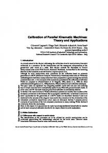
5. Case Study We take the generic structure for a kinematic analysis and design optimization. 5.1. FORWARD KINEMATICS Forward kinematics is to determine the end-effector motion when the actuated joint motions ui (i=1, 2, 3) are known. To solve the problem of the forward kinematics, the middle variable ϕi (i=1,2,3), which represents an angle between supporting bar DiEi and the base platform B1B2B3 in Figure 6, is introduced. Note that once ϕi is calculated from given ui, the posture of the end-effector can be easily derived.
Figure 3: Reconfigurable 5-axis Parallel Kinematic Machine (Horizontal case)
By expressing the coordinate of Ei with respect to {Obxbybzb} in terms of ui and ϕi, and considering the constraint equations Ei E j = 3le , one has:
K ij cϕ i cϕ j + Lij sϕ i sϕ j + M ij cϕ i + N ij cϕ j
Similarly for an arbitrary ϕ2, we have the formula c 2ϕ 2 + s 2ϕ 2 = 1 . Substituting equation (3) into this formula gets:
+ Oij sϕ i + Pij sϕ j + Qij = 0
(i, j = 1,2,3,
i ≠ j)
V3 s 2ϕ 2 + V2 sϕ 2 + V1 = 0
(1) where c and s represent the cosine and sine functions, respectively. K ij , Lij , M ij , N ij , Oij , Pij , Qij are the coefficients related to the structural parameters and the joint motion ui. fe
μe
E3 H3
U 12V32 − U 1U 2V2V3 + V1V3U 22 + U 1U 3V22 ye
E2 le Oe E1
ϕi
− 2U 1U 3V1V3 − U 2U 3V1V2 + U 32V12 = 0
H2
(6) Equation (6) has only ϕ3 unknown. Therefore, ϕ3 can be obtained by employing the numerical algorithm. After ϕ3 is calculated from equation (6), ϕ2 and ϕ1 can be calculated from (4) or (5), and from (2), sequentially.
xe H1
zb
D3
D2 yb
D1 ui
To reach a meaningful solution, equation (4) and (5) must be satisfied simultaneously, and this results in a necessary and sufficient condition:
ze
βi
li
(5) where Vi (i=1,2,3) are the coefficients related to the structure parameters, the joint motion ui, and ϕ3.
γi αi B3
lb
When ϕi (i=1,2,3) is known, the coordinate of Ei with respect to {Ob-xbybzb} can be calculated, and the posture of the end-effector is then determined by:
B2 xb
Ob B1
Figure 6: Schematic representation
⎡R p ⎤ ⎡xe ye ze pe ⎤ Te = ⎢ e e ⎥ = ⎢ ⎥= ⎣ 0 1⎦ ⎣0 0 0 1⎦ ⎡ re − re / 3le 2re2 − re1 − re3 /(3le ) re1 − re3 × re2 − re1 / 3le2 ⎢ 1 3 ⎢⎣ 0 0 0
(
Equation (1) includes three independent equations with respect to ϕi (i=1,2,3). Using two of them, one can represent ϕ1 is terms of ϕ2 and ϕ3, cϕ 1 = (R1 cϕ 2 + S 1 sϕ 2 + T1 ) / (R 2 cϕ 2 + S 2 sϕ 2 + T2 ) ⎫ ⎬ sϕ 1 = −(R3 cϕ 2 + S 3 sϕ 2 + T3 ) / (R 2 cϕ 2 + S 2 sϕ 2 + T2 )⎭ (2) where Ri,Si,Ti (i=1,2,3) are the coefficients related to the structure parameters, the joint motion ui, and ϕ3. Substituting equation (2) into independent equation of (1) obtains:
the
remaining
)( ) (
)
(
)(
) ( ) (r
e1
)
+ re2 + re3 / 3⎤ ⎥ ⎥⎦ 1
(7) where Te is the posture of the end-effector with respect to {Ob-xbybzb}. Re=(xe, ye, ze) and pe represent the orientation and the position of the end-effector, respectively. rei (i=1,2,3) are the coordinates of Ei with respect to {Ob-xbybzb}. 5.2. INVERSE KINEMATICS
L sϕ + O23 N cϕ + P23 sϕ 3 + Q23 cϕ 2 = − 23 3 sϕ 2 − 23 3 K 23 cϕ 3 + M 23 K 23 cϕ 3 + M 23
(3) Note that for an arbitrary ϕ1, the formula c 2ϕ1 + s 2ϕ1 = 1 is always satisfied. Using equation (2) in the formula, and substituting cϕ2 by equation (3) results in, U 3 s 2ϕ 2 + U 2 sϕ 2 + U 1 = 0 (4) where Ui (i=1,2,3) are the coefficients related to the structural parameters, the joint motion ui, and ϕ3.
Inverse kinematics determine the joint motions when the end-effector motion is known. The motion of the end-effector is specified by its three independent motions: x and y rotation, and z translation. However, the posture of the end-effector, Te in equation (7), must be fully described by the three rotational parameters (θ x , θ y , θ z ) and three translational parameters
(x e , y e , z e ) as:
cθycθz sθy −cθysθz ⎡ ⎡Re pe ⎤ ⎢⎢ sθxsθycθz +cθxsθz −sθxsθysθz +cθxcθz −sθxcθy Te =⎢ ⎥= ⎣ 0 1 ⎦ ⎢−cθxsθycθz +sθxsθz cθxsθysθz +sθxcθz cθxcθy ⎢ 0 0 0 ⎣
(9)
ui∈[0.05m, 0.5m]. The ranges of other parameters are given as Table 1. The optimization is based on a Genetic Algorithm (GA) approach. However, the structural parameters in the optimized result are given in the second row of Table 1. The result shows that the radius of the base platform should be equal to that of the movable platform, and it should be as small as possible. The length of a supporting bar has a great impact on both of the rotational motion of the endeffector and the deformation of the supporting bar. A longer supporting bar results in relatively large rotational motion of the end-effector but greater deformation of the supporting bar. A trade-off of these impacts is therefore required to determine the length.
(10)
Table 1: Ranges and optimal values of design parameters
xe ⎤ ye ⎥⎥ ze ⎥ ⎥ 1⎦
(8) When
(θ
x
,θ y , z e )
are selected as independent
parameters, the remainder (x e , y e , θ z ) are dependant parameters. The dependence of these parameters can be found based on the fact that Ob Bi Di E i (i=1,2,3) is within the co-plane [15], thus: ⎛ − sθ x sθ y ⎜ cθ + cθ y ⎝ x
θ z = tan −1 ⎜
⎞ ⎟ ⎟ ⎠
x e = − 3l e cθ yθ z / 3
y e = 3l e (cθ x cθ z − cθ y cθ z − sθ x sθ y sθ z ) / 6
γ
As a result, when the end-effector motion is specified by (θ x ,θ y , ze ) , the posture of the end-effector is totally determined. Further, the joint motions can be derived from the constraint of fixed length for the supporting bar:
(i = 1,2,3)
Ob E i − O b B i − B i D i = D i E i
(12)
Equation (12) further gives ui =
− k b ± k b2 − 4k c
lb(m)
le(m)
li(m)
[91, 150]
[0.2, 0.7]
[0.2, 0.7]
[0.2, 0.7]
107.329628
0.204105
0.200000
0.692329
(degree)
(11) Range Optimal value
Figure 7 shows the workspace of the optimized tripod. The motion range of the z-translation is (0.7398m, 1.1525m). The motion ranges of x-and y- rotations are about ±45º. There is no void or hole within the workspace.
(13)
2
where
[ (
)
kb = 2 cγ xei cα i + yei sα i − lb − zei sγ
]
⎫⎪ ⎬ kc = x + y + z + l − l − 2lb xei cα i + yei sα i ⎪⎭ 2 ei
⎡xebi ⎤ ⎡xeei ⎤ ⎢ b⎥ ⎢ ⎥ Pei = ⎢yei ⎥ = Re ⋅ ⎢yeei ⎥ + pe ⎢zeb ⎥ ⎢zee ⎥ ⎣ i⎦ ⎣ i⎦
2 ei
2 ei
2 b
2 i
(
)
=
⎡ ⎤ lecβicθycθz − lesβicθysθz + xe ⎢ ⎥ ( ) ( ) + + − + + l c β s θ s θ c θ c θ s θ l s β s θ s θ s θ c θ c θ y x z e i x y z x z e⎥ ⎢e i x y z ⎢lecβi (− cθxsθycθz + sθxsθz ) + lesβi (cθxsθysθz + sθxcθz ) + ze ⎥ ⎣ ⎦
5.3 DESIGN OPTIMINZATION Using the developed kinematic model, the structural parameters can be optimized in the sense that the rotational motion of the end-effector can be maximized. In the optimization, the actuated prismatic joints are assumed to be off-the-shelf components, and the motion ranges of these joints are known as
Figure 7: Workspace of the optimized structure
6. CONCLUSIONS This paper presents a series of novel reconfigurable parallel kinematic machines using modular design methodology. The conceptual design of this type of
machine is introduced, and the detail configurations of potential structures are showed. A case study for the generic case is conducted, forward and inverse kinematic models have been established. Using these models, the design and simulation have been performed. The results have illustrated that this type of reconfigurable kinematic machine can achieve a large workspace without a void or a hole, and it has no interference among the system components.
ACKNOWLEDGEMENTS: The first author acknowledges the support for this work provided by the Natural Sciences and Engineering Research Council of Canada (NSERC) and Kayla Viegas for the CAD models. REFERENCES 1.
R.Cohen,et al.,1992, Conceptual design of a modular robot, ASME J. Mechanical Design, 112,117-125. 2. R.Harrison et al., 1986, Industrial application of pneumatic servo-controlled modular robots, Proc. 1st National Conf. on Production Research, 229-236. 3. R.Hooper and D.Tesar, 1994, Computer-aided configuration of modular robotic systems, J. of Computing & Control Engineering, 137-142. 4. K.H.Wurst, 1986, The conception and construction of a modular robot system, Proc. of Int. Symp. on Industrial Robotics, Belgium, 37-44. 5. K.H.Wurst, 1991, Flexible robot system - conception and realisation of modular robot components (in German), PhD dissertation, University of Stuttgart, Springer-Verlag. 6. W.L.Xu, G. Pritschow and K.H. Wurst, 1994, Transmission error of a modular robotic joint, JSME Int. J. Ser.C, Dynamics, Control, Robotics, Design and Manufacturing, 37(4), 765-773. 7. W.L.Xu, K.H. Wurst and S.Q.Yang, 1994, Calibrating a modular robot joint using neural network, IEEE Int. Conf. on Neural Networks, Florida, USA, 2720-2725. 8. Pradeep K. Khosla, et al., 1988, The Carnegie Mellon Reconfigurable Modular Manipulator System Project, Annual Report, The Robotics Institute, Carnegie Mellon University, USA. 9. S. Postma, 1988, Modular robots for flexible production automation, Technical Report, V-5.9.S.7, TU Delft, The Netherlands. 10. D. Tesar and M.S. Butler, 1989, A generalised modular architecture for robot structures, J.of Manufacturing Review, 2(2), 91-118. 11. Hunt, K. H., 1978, Kinematic Geometry of Mechanisms, Clarendon, Press, Oxford 12. Zhang, D. (2000). Kinetostatic Analysis and Optimization of Parallel and Hybrid Architectures for Machine Tools, Ph.D. Thesis, Laval University, Canada