Development of Response Surface Equations for High ... - CiteSeerX

975570

Development of Response Surface Equations for High-Speed Civil Transport Takeoff and Landing Noise Erik D. Olson and Dr. Dimitri N. Mavris Georgia Institute of Technology Copyright © 1997 Society of Automotive Engineers, Inc.

ABSTRACT As an element of a design optimization study of high speed civil transport (HSCT), response surface equations (RSEs) were developed with the goal of accurately predicting the sideline, takeoff, and approach noise levels for any combination of selected design variables. These RSEs were needed during vehicle synthesis to constrain the aircraft design to meet FAR 36, Stage 3 noise levels. Development of the RSEs was useful as an application of response surface methodology to a previously untested discipline. Noise levels were predicted using the Aircraft Noise Prediction Program (ANOPP), with additional corrections to account for inlet and exhaust duct lining, mixer-ejector nozzles, multiple fan stages, and wing reflection. The fan, jet, and airframe contributions were considered in the aircraft source noise prediction. Since takeoff and landing noise levels are a function of both engine design variables and flight path variables, several possible approaches to the problem were considered. The first method would have required developing an RSE which is a function of low-speed aerodynamics and engine design variables, by using the Flight Optimization System (FLOPS) computer program to calculate the takeoff performance and passing the flight path to ANOPP. The second method required development of an RSE which is a function of engine cycle variables and flight path variables. The latter approach was chosen for this study, primarily for its simplicity and ease of integration of the final RSEs into FLOPS. Pareto plots are provided showing the estimated effect of each of the variables on the variation in the noise levels. Screening studies showed that the variation in sideline noise was dominated by jet parameters--such as mass flow, area, total pressure, and suppressor area ratio--while fan variables and climb velocity played a smaller role. Takeoff noise was similarly affected, except that the sensitivity to the jet variables was diminished, and cutback altitude was shown to have a significant effect. Approach noise was controlled almost completely by fan variables. The most important variables were chosen for each of the three noise levels, and separate response surface equations were developed for two-, three-, and four-stage fans using a central composite design of

experiments (CCD) matrix. The resulting RSE coefficients are given, along with plots for the prediction profiles for each equation. The sideline and takeoff noise RSEs all exhibited good fit with the data, and the trends were as expected. The approach noise RSEs exhibited lower R2 values, indicating a poorer fit with the data. It was determined that this behavior was caused by correlation in the design matrix, resulting in significant errors in the estimation of the second-order RSE coefficients. Problems with the approach RSEs were eliminated when their development was repeated using a face-centered form of the CCD. Based on the results of this study, recommendations are made for any future studies in this area. INTRODUCTION In the Aerospace Systems Design Laboratory at Georgia Tech, a new design methodology is in the process of development which can be described as a Concurrent Engineering approach to aerospace design applied in an Integrated Product and Process Development environment. Under the proposed environment it becomes much harder to separate the traditional ideas of conceptual and preliminary design. To facilitate true multidisciplinary analysis at an earlier phase in the design cycle, a methodology for determination of economically robust design solutions called Robust Design Simulation (RDS)1 is employed. RDS replaces historically-derived empirical databases with physicsbased disciplinary analysis, and is based on a probabilistic approach to aerospace systems design, which views the chosen objective as a distribution function introduced by uncertainty variables. 2 The procedure employs the use of design of experiments (DOE) to facilitate the development of response surface equations (RSEs) which approximate sophisticated, computationally intense disciplinary analysis tools with second-order polynomial equations. After RSEs are generated for each of the disciplines--aerodynamics, structures, propulsion, etc.--they are then integrated into a sizing and synthesis tool for system-level studies. At this level, a very large number of rapid cases can be run using the RSEs to provide preliminary-level disciplinary analysis without the large associated computation times.

The ability to generate a large number of results allows for a probabilistic approach to the estimation of systemlevel metrics using Monte Carlo or Fast Probability Integration methods. In this manner, the effects of economic uncertainty as well as discipline, technology, and schedule risk can be included in the risk analysis of the system. This study details a portion of a graduate design study conducted at Georgia Tech aimed at applying the RDS methodology to the high-speed civil transport (HSCT) aircraft. The objective of the takeoff and landing noise portion of this project was to develop a set of response surface equations to accurately predict the sideline, takeoff, and approach noise levels of any configuration within the design space using any anticipated set of takeoff procedures. The RSEs could then be used as design constraints to ensure that the aircraft was capable of meeting the required certification noise levels. Since Response Surface Methodology (RSM) has not previously been applied to the area of takeoff and landing noise prediction, the development of noise RSEs was useful as a demonstration of the methodology applied to a relatively simple noise prediction program. RESPONSE SURFACE METHODOLOGY RSM is composed of a number of statistical techniques for empirically relating an output variable, or response, to the levels of a number of input variables 2. RSM serves to provide a simple model spanning the entire design space for a complex model for which no analytical solution exists by simplifying the relationships into a polynomial equation. In this study, a second-degree model was used, of the form n

n

i =1

i =1

n −1

n

R = b 0 + ∑ b i x i + ∑ b ii x 2i + ∑ ∑ b ijx i x j

(1)

i =1 j = i +1

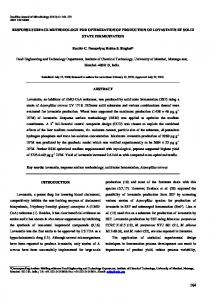
where b 0 is the intercept, bi are regression coefficients for the linear terms, bii are regression coefficients for the pure quadratic terms, and bij are regression coefficients for the cross-product terms. The x i variables represent the normalized values of each of the input variables which affect the response. An illustration of a simple two-variable RSE is shown in Figure 1. The RSE provides a simple polynomial equation which can be used in lieu of more sophisticated, time-consuming computations to predict the value of the response for any combination of input values. The most common method of obtaining the regression coefficients is through design of experiments, which provides an efficient and methodical system for determining the necessary combinations of factor levels for obtaining the maximum regression information with a minimum number of runs. Table 1 illustrates a simple

x2 x1

Figure 1: Graphic depiction of a two-variable response surface equation2 two-level, full-factorial DOE table for three design variables. In this case the variables take on one of two levels, either minimum or maximum, which are normalized to -1 and +1. The DOE table then indicates which combinations of factor levels are required for each of the eight runs. Table 1: Example Full-Factorial DOE Table for Three Variables 3

Run 1 2 3 4 5 6 7 8

x1 -1 +1 -1 +1 -1 +1 -1 +1

Factors x2 -1 -1 +1 +1 -1 -1 +1 +1

x3 -1 -1 -1 -1 +1 +1 +1 +1

Response y1 y2 y3 y4 y5 y6 y7 y8

Since the factors in this model only take on one of two levels, only linear terms in the RSE can be estimated. To use the quadratic RSE model as given in Equation 1, it is necessary to use a three- or higher-level design of experiments. However, increasing the number of levels for each variable causes the number of cases required to increase rapidly. Table 2 shows that for more than a handful of variables, the number of runs quickly becomes impractical for the full-factorial model. To reduce the number of runs required without eliminating any variables, it is necessary to use a fractional-factorial design or one of a number of designs which are specially created to minimize the total number of runs. The total number of runs required is greatly reduced, but at the expense of a decrease in the number of regression coefficients which can be estimated. The type of DOE used in this study was the centralcomposite design (CCD). A CCD formulation retains the Table 2: Number of Cases for Different DOEs3 DOE 3-level, Full Factorial Central Composite Box-Behnken D-Optimal

7 Variables 2187 143 62 36

12 Variables 531441 4121 2187 91

Equation 3n 2n+2n+1 (n+1)(n+2)/2

Figure 4: Observer locations for FAR 36 certification. The sideline observer is located along the sideline at the point where the noise level is greatest5. located along the centerline, at a point 6562 feet before the landing threshold. Once the noise levels at the three observers are measured, they are converted into an effective perceived noise level (EPNL) which represents a single number rating the annoyance of the entire flight procedure to a person at that location. EPNL includes frequency weighting, correction for any tones which protrude above the rest of the spectrum and thus are more noticeable, and a time averaging to account for the duration of the noise event. The calculated EPNL values are then compared to the Stage 3 limits shown in Figure 5 to determine whether the aircraft can be certified. Typical noise limits are indicated on the figure for an HSCT. AIRCRAFT NOISE PREDICTION METHODOLOGY The Aircraft Noise Prediction Program (ANOPP) is a NASA-Langley program which was originally developed, and is constantly updated, to provide noise prediction with the best publicly available methods 6. ANOPP uses empirical predictions of each of the separate noise components in the engine and airframe, combined with physical models of propagation, atmospheric absorption,

Figure 6: Cross-section of a laminar liner A cutaway diagram of a mixer-ejector nozzle is shown in Figure 8. To account for the suppression of jet noise by mixer-ejector nozzles, data from reference 10 was used to obtain curve fits for the amount of secondary air which is entrained into the ejector as a function of the suppressor area ratio (SAR) and the nozzle pressure ratio (NPR). The SAR is defined as the ratio of the total nozzle area, including the ejector, to the area of just the primary nozzle:

Figure 9: Effect of NPR and SAR on the suppression of a mixer-ejector nozzle AUTOMATION OF NOISE ANALYSIS - To use ANOPP in a design of experiments environment, it was necessary to create an automation routine as shown in Figure 10. An execution control program was created to accept the DOE matrix created by the JMP program12, then use a list of variable ranges to set the ANOPP input parameters to the necessary values. Variables not referenced by the DOE matrix were set to their default values. The data were then written as an input file for the ANOPP preprocessor, and the control program would run the pre-processor and ANOPP, then pass the data to the ANOPP post-processor for extraction of EPNL data.

Figure 11: Ishikawa diagram for sideline, takeoff, and approach EPNL

Table 3: Component Noise Source Prediction Methods

Noise Source Fan and Compressor

Core and Turbine Jet Airframe Propagation

Prediction Method Heidmann w/ multistage modifications rotor-stator interaction tones broadband combination tones inlet flow distortion inlet guide vanes none SAE Single-Stream mixing only Fink w/ delta wing option all components included SAE absorption Chien-Soroka ground effects no lateral attenuation

rotor-stator interaction tones, broadband noise, combination tones, inlet flow distortion, and inlet guide vanes were all included in the fan noise prediction. The effect of multiple stages was accounted for by calculating the noise levels of the individual stages and then superimposing the separate noise levels. The number of vanes was chosen, based on the number of blades, to achieve cutoff of the blade passing frequency for each engine configuration. Inlet and exhaust liner depths were chosen to tune the liner to the bladepassing frequency, and the inlet noise was increased by 2 dB to account for wing reflection. Airframe noise was predicted using the Fink method with the delta wing option. Finally, atmospheric absorption was calculated using the SAE standard absorption method, with ground effects but no extra lateral attenuation.

Figure 12: Flight path decomposition into sideline, takeoff, and approach flight path segments GROUND RULES AND ASSUMPTIONS - The engine source noise was assumed to consist of the fan, jet, and airframe components (Table 3). Turbine noise was not included in the calculations because past experience with ANOPP's turbine noise module has shown it to over-predict turbine noise, resulting in extremely high levels which tend to drown out the other noise sources. In addition, the core noise levels were not included since attempts to include them also resulted in unexpectedly high noise levels. Experience with previous HSCT systems studies has shown that the fan and jet sources are dominant. The fan source noise levels were predicted using the Heidmann fan noise module. The individual effects of

The predicted noise levels for the baseline aircraft are shown in Figure 13, including the effects of fan inlet and exhaust lining, an SAR of 3.7, and wing reflection of inlet noise. The dominant noise sources for sideline and takeoff are the jet and fan components, while the airframe levels contribute almost nothing to the total EPNL. For approach, the noise levels are dominated by the fan, with airframe and jet components having a very small effect. To account for changes in engine component size as the engine size varied, the area of each of the components was assumed to vary directly with the engine mass flow; and the diameters were assumed to vary with the square root of the mass flow. Since the number of fan stages was allowed to vary, it was impractical to include the area, diameter, number of blades, etc. for each of the fan stages. For a two-stage fan, this would have resulted in nonexistent values for the third and fourth stage geometric parameters. To get around this problem, it was assumed that the ratio of the area of the second stage to the area of the first stage was constant, and that the ratio of the number of fan blades and stators

115 110 105

EPNL

100

Total Fan Inlet Fan Exhaust Jet Airframe

95 90 85 80 75 70 Approach

Sideline

Takeoff

Figure 13: Predicted FAR 36 noise levels for the HSCT baseline (SAR = 3.7) from one stage to the next was likewise constant. The first-stage fan diameter was also eliminated as a variable by assuming a constant hub diameter ratio for each of the stages, resulting in a unique relation between the area and diameter of each stage. In addition, the rotorstator spacing was assumed constant over all stages, and the total fan compression was assumed to be divided equally among each of the stages. In addition to the assumptions made in decomposing the flight path, it was assumed that the all FAR 36 regulations would be adhered to completely, precluding the use of programmed throttle reductions below the minimum cutback altitude or the use of accelerating climb procedures. This assumption also precluded the use of high-angle or two-stage approach procedures. VARIABLE SCREENING - Table 4 gives the list of twenty variables which were chosen for consideration as

parameters in the sideline, takeoff and approach noise RSEs. Also given are the minimum and maximum values which the variables were expected to take throughout the design space. The ranges for the flight path variables were chosen based on the estimated maximum variation of each parameter from the values for the baseline aircraft. The throttle setting was assumed to vary between 80% and 100% for the sideline flight segment, 50% and 80% for the takeoff segment, and 15% to 23% for approach. The resulting ranges for each of the engine operating conditions were derived using the assumed ranges for the throttle settings, combined with the ranges for each of the engine design variables. For example, the minimum sideline fan mass flow rate in Table 4 results from the minimum design inlet mass flow at the minimum sideline throttle setting; while the maximum fan mass flow is calculated from the maximum inlet mass flow at the maximum throttle setting. Fan geometries were scaled with engine size as discussed previously, and the ranges for the inlet and exhaust liner lengths were estimated from the range of overall engine lengths being studied. Rotor-stator spacing was varied from 30 to 100% to assess the benefits of designing the engine with increased spacing as a noise control measure. Similar methods were used to determine the ranges for the jet noise variables. The range for SAR was chosen from the range of values studied in references 9 and 10.

Table 4: Variables and Ranges Prior to Screening

Flight Path Velocity, kt Flight path angle, deg Angle of attack, deg Cutback altitude, ft Fan Noise Mass flow, lbm/sec Rotation speed, RPM Temperature rise, §R Number of stages 1st stage area, ft2 1st stage rotor blades Rotor-stator spacing, % 1st stage design Mtip Inlet duct lined length, ft Exhaust lined length, ft Jet Noise Mass flow, lbm/sec Total pressure, psf Total temperature, §R Throat area, ft2 Fuel/air ratio Nozzle SAR

Sideline 180 4 8 --

Takeoff 220 9 14 --

Sideline 450 780 3750 5170 193.4 295.4 2 4 19.7 24.1 22 36 30 100 0.9 1.1 1.9 2.3 6.7 8.2 Sideline 427 760 6350 9530 1750 2100 6.6 10.6 0.018 0.022 2.7 4.7

180 4 8 1350

Approach 220 9 14 1950

Takeoff 365 3400 140.6 2 19.7 22 30 0.9 1.9 6.7

700 5000 259.8 4 24.1 36 100 1.1 2.3 8.2

Takeoff 335 4450 1460 5.8 0.017 2.7

678 8040 1930 9.9 0.021 4.7

140 -3 8 --

165 -3 14 --

Approach 225 402 3100 4350 79.3 121.8 2 4 19.7 24.1 22 36 30 100 0.9 1.1 1.9 2.3 6.7 8.2 Approach 228 392 2750 3810 1110 1300 5.6 8.2 0.015 0.019 2.7 4.7

Figure 16: Pareto screening plot for approach EPNL attitude during approach results in the aircraft being closer to or farther from the observer when the observation angle results in the greatest noise. Based on the results of the screening test, eight variables were chosen for use in the approach noise RSE. RESPONSE SURFACE EQUATION DEVELOPMENT For all three screening tests, the number of fan stages was one of the important variables chosen. Due to the discrete nature of this variable, and due to that fact that it only takes three values--two, three, or four-- it could not be included in the RSEs as a continuous variable since the star points are located at real-valued points. As a result, separate RSEs had to be created for each value for the number of fan stages, resulting in three times as many RSEs and three times as many runs. The number of fan blades was also a discrete variable, but it had 15 levels (22 to 36), so it could be approximated by a continuous variable. Ten sideline variables were used, resulting in 149 runs per RSE using a rotatable centralcomposite design matrix. For takeoff EPNL, 11

Figure 17: Prediction profiles for sideline EPNL

Figure 19: Prediction profiles for approach EPNL

Table 8: Selected Results from Verification Runs

RSE Sideline Sideline Sideline Takeoff Takeoff Takeoff Approach Approach Approach

No. Stages 2 3 4 2 3 4 2 3 4

Predicted 111.39 119.27 98.75 98.26 118.4 104.42 112.95 106.2 99.85

Actual 111.46 118.24 100.7 100.2 116.43 104.39 113.84 106.11 99.84

Error -0.07 1.03 -1.95 -1.94 1.97 0.03 -0.89 0.09 0.01

For the final RSEs that were generated, the model fits were good for all three observers. After initially developing the approach RSEs with a rotatable CCD, the severe overestimation of the quadratic effects of each variable made it necessary to reevaluate the RSEs using a face-centered design. In this study, it was possible to repeat the entire process because each of the runs was relative inexpensive in terms of computational time. However, for a true physics-based, computationally intensive noise prediction model, this would not be the case. Unfortunately, there may be no easy way of determining beforehand whether a given value of α for the CCD will result in a good fit. It is possible that the original flawed approach RSEs could have been improved by eliminating the quadratic terms in the equation for those variables which are known to have only a linear response; these modifications, however, would require a good knowledge of the sensitivity of the response to the different variables, and would run the risk of mistakenly eliminating quadratic effects that are actually significant. While the RSEs were able to account for the effects of nozzle suppression and rotor-stator spacing on the noise, no method was available for predicting the associated nozzle and engine weight increases. These would be needed to determine the performance penalties associated with meeting the noise requirements. This study has served as a test case for the generation of noise RSEs as part of an integrated robust design study using an empirically-based noise prediction program which is relatively inexpensive computationally. The true application of response surface methodology, however, lies in the ability to approximate the results from more accurate, computationally intensive models. Further research is being conducted to test the application of response surface methodology to higherorder, physically-based methods of noise analysis. Also, although only FAR 36 noise levels were considered in this study, similar methods could be used to generate RSEs for other noise concerns such as airport community noise contour areas, climb-to-cruise noise, or sonic boom. These problems were too complex to be studied in the available time.

REFERENCES 1.

Mavris, D., Bandte, O., and Brewer, J.: A Method for the Identification and Assessment of Critical Technologies Needed for an Economically Viable HSCT. 1st AIAA Aircraft Engineering, Technology, and Operations Congress, Los Angeles, CA, September 19-21, 1995. 2. DeLaurentis, D., Mavris, D., and Schrage, D.: System Synthesis in Preliminary Aircraft Design Using Statistical Methods. 20th Congress of the International Council of the Aeronautical Sciences, Sorrento, Italy, Sept. 8-13, 1996. 3. Box, G. E. P., and Draper, N. R., Empirical Model-Building and Response Surfaces , John Wiley & Sons, Inc., New York; 1987. 4. DOT/FAA Noise Standards: Aircraft Type and Airworthiness Certification, FAR Part 36, January 1, 1990. 5. Olson, E. D.: Advanced Takeoff Procedures for HighSpeed Civil Transport Commu nity Noise Reduction. SAE Aerotech ‘92, October, 1992. 6. Zorumski, William E.: Aircraft Noise Prediction Program Theoretical Manual. NASA TM-83199, 1982. 7. Clark, Bruce J.: Computer Program to Predict Aircraft Noise Levels. NASA TP-1913, September, 1981. 8. McCullers, L. A. Flight Optimization System User’s Guide, Version 5.7, NASA Langley Research Center, 1995. 9. Kershaw, R.J., and House, M.E.: Sound-Absorbent Duct Design. Noise and Vibration. White, R.G., and Walker, J.G., ed. New York: John Wiley & Sons, 1982. 10. Stern, Alfred M.: HSCT Nozzle Source Noise Programs at Pratt & Whitney. NASA First Annual High Speed Research Workshop, May 14-16, 1991. NASA CP-10087. 11. Choi, Y. H., and Soh, W. Y.: Computational Analysis of the Flowfield of a Two-Dimensional Ejector Nozzle. NASA CR185255, 1990. 12. SAS Institute, Inc.: JMP Computer Program and User’s Manual, Cary, NC, 1994.