Development of Seismic Vulnerability Assessment ... - CiteSeerX

ISET Journal of Earthquake Technology, Paper No. 472, Vol. 43, No. 3, September 2006, pp. 75-104

DEVELOPMENT OF SEISMIC VULNERABILITY ASSESSMENT METHODOLOGIES OVER THE PAST 30 YEARS G.M. Calvi*, R. Pinho**, G. Magenes*, J.J. Bommer***, L.F. Restrepo-Vélez**** and H. Crowley** *Department of Structural Mechanics, University of Pavia, Pavia, Italy **European Centre for Training and Research in Earthquake Engineering (EUCENTRE), Pavia, Italy ***Department of Civil and Environmental Engineering, Imperial College London, U.K. ****Solingral S.A., Medellin, Colombia

ABSTRACT Models capable of estimating losses in future earthquakes are of fundamental importance for emergency planners and for the insurance and reinsurance industries. One of the main ingredients in a loss model is an accurate, transparent and conceptually sound algorithm to assess the seismic vulnerability of the building stock and indeed many tools and methodologies have been proposed over the past 30 years for this purpose. This paper takes a look at some of the most significant contributions in the field of vulnerability assessment and identifies the key advantages and disadvantages of these procedures in order to distinguish the main characteristics of an ideal methodology. KEYWORDS:

Vulnerability Assessment, Loss Estimation, Unreinforced Masonry, Reinforced Concrete

INTRODUCTION In the last few decades, a dramatic increase in the losses caused by natural catastrophes has been observed worldwide. Reasons for the increased losses are manifold, though these certainly include the increase in world population, the development of new “super-cities” (with a population greater than 2 million), many of which are located in zones of high seismic hazard, and the high vulnerability of modern societies and technologies (e.g., Smolka et al., 2004). The 1994 Northridge (California, US) earthquake produced the highest ever insured earthquake loss at approximately US$14 billion, and the US$150 billion cost of the 1995 Kobe (Japan) earthquake was the highest ever absolute earthquake loss. Although the dollar value of economic losses in other parts of the world may be far lower than in Japan and the US, the impact on the national economy may be much greater due to losses being a larger proportion of the gross national product (GNP) in that year. Coburn and Spence (2002) report the economic losses due to earthquakes from 1972 to 1990; the three largest losses as proportions of the GNP are in the Central American countries of Nicaragua (1972, 40% GNP), Guatemala (1976, 18% GNP) and El Salvador (1986, 31% GNP). When the economic burden falls entirely on the government (such as occurred after the 1999 Kocaeli earthquake in Turkey), the impact on the national economy can be crippling; one possible solution is to privatise the risk by offering insurance to homeowners and then to export large parts of the risk to the world’s reinsurance markets (e.g., Bommer et al., 2002). In order to design such insurance and reinsurance schemes, a reliable earthquake loss model for the region under consideration needs to be compiled such that the future losses due to earthquakes can be determined with relative accuracy. The formulation of an earthquake loss model for a given region is not only of interest for predicting the economic impact of future earthquakes, but can also be of importance for risk mitigation. A loss model that allows the damage to the built environment and important lifelines to be predicted for a given scenario (perhaps the repetition of a significant historical earthquake) can be particularly important for emergency response and disaster planning by a national authority. Additionally, the model can be used to mitigate risk through the calibration of seismic codes for the design of new buildings; the additional cost in providing seismic resistance can be quantitatively compared with the potential losses that are subsequently avoided. Furthermore, the loss model can be used to design retrofitting schemes by carrying out cost/benefit studies for different types of structural intervention schemes. Earthquake loss models should, ideally, include all of the possible hazards from earthquakes: amplified ground shaking, landslides, liquefaction, surface fault rupture, and tsunamis. Nevertheless,

76

Development of Seismic Vulnerability Assessment Methodologies over the Past 30 Years

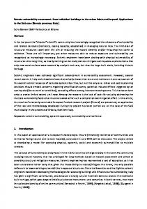
strong ground shaking is often the only hazard considered in loss assessment methods; this is commonly an acceptable approach because as the size of the loss model increases, the relative influence of the secondary hazards such as liquefaction and landslides decreases (Bird and Bommer, 2004). Constructing an earthquake loss model for a city, region or country involves compiling databases of earthquake activity, ground conditions, ground-motion prediction equations, building stock and infrastructure exposure, and vulnerability characteristics of the exposed inventory. The main aim of a loss model is to calculate the seismic hazard at all the sites of interest and to convolve this hazard with the vulnerability of the exposed building stock such that the damage distribution of the building stock can be predicted; damage ratios, which relate the cost of repair and replacement to the cost of demolition and replacement of the structures, can then be used to calculate the loss. A significant component of a loss model is a methodology to assess the vulnerability of the built environment. The seismic vulnerability of a structure can be described as its susceptibility to damage by ground shaking of a given intensity. The aim of a vulnerability assessment is to obtain the probability of a given level of damage to a given building type due to a scenario earthquake. The various methods for vulnerability assessment that have been proposed in the past for use in loss estimation can be divided into two main categories: empirical or analytical, both of which can be used in hybrid methods (see Figure 1). Scenario Earthquake

Ground Motion Characterisation

Damage Scale

Vulnerability Assessment Method

Empirical

Damage Probability Matrix

Typological

Field Survey

Analytical

Hybrid

Vulnerability Functions

Expert Judgement

Collapse Mechanism Based

Capacity Spectrum Based

Fully Displacement Based

Ratio between cost of repair and cost of replacement for the whole building stock

Fig. 1

The components of seismic risk assessment and choices for the vulnerability assessment procedure; the bold path shows a traditional assessment method

ISET Journal of Earthquake Technology, September 2006

77

A vulnerability assessment needs to be made for a particular characterisation of the ground motion, which will represent the seismic demand of the earthquake on the building. The selected parameter should be able to correlate the ground motion with the damage to the buildings. Traditionally, macroseismic intensity and peak ground acceleration (PGA) have been used, whilst more recent proposals have linked the seismic vulnerability of the buildings to response spectra obtained from the ground motions. Each vulnerability assessment method models the damage on a discrete damage scale; frequently used examples include the MSK scale (Medvedev and Sponheuer, 1969), the Modified Mercalli scale (Wood and Neumann, 1931) and the EMS98 scale (Grünthal, 1998). In empirical vulnerability procedures, the damage scale is used in reconnaissance efforts to produce post-earthquake damage statistics, whilst in analytical procedures this is related to limit-state mechanical properties of the buildings, such as interstorey drift capacity. The evolution of vulnerability assessment procedures for both individual buildings and building classes is described in the following sections, wherein the most important references, applications and developments pertaining to each methodology are reported. A larger emphasis has been placed on the vulnerability assessment of the built environment at an urban scale for use in risk and loss assessment methodologies. EMPIRICAL METHODS As described below, the seismic vulnerability assessment of buildings at large geographical scales has been first carried out in the early 70’s, through the employment of empirical methods initially developed and calibrated as a function of macroseismic intensities. This came as a result of the fact that, at the time, hazard maps were, in their vast majority, defined in terms of these discrete damage scales (earlier attempts to correlate intensity to physical quantities, such as PGA, led to unacceptably large scatter). Therefore these empirical approaches constituted the only reasonable and possible approaches that could be initially employed in seismic risk analyses at a large scale. There are two main types of empirical methods for the seismic vulnerability assessment of buildings that are based on the damage observed after earthquakes, both of which can be termed “damage-motion relationships”: 1) damage probability matrices (DPM), which express in a discrete form the conditional probability of obtaining a damage level j , due to a ground motion of intensity i , P  D = j i  ; and 2) vulnerability functions, which are continuous functions expressing the probability of exceeding a given damage state, given a function of the earthquake intensity. 1. Damage Probability Matrices Whitman et al. (1973) first proposed the use of damage probability matrices for the probabilistic prediction of damage to buildings from earthquakes. The concept of a DPM is that a given structural typology will have the same probability of being in a given damage state for a given earthquake intensity. The format of the DPM suggested by Whitman et al. (1973) is presented in Table 1, where example proportions of buildings with a given level of structural and non-structural damage are provided as a function of intensity (note that the damage ratio represents the ratio of cost of repair to cost of replacement). Whitman et al. (1973) compiled DPMs for various structural typologies according to the damaged sustained in over 1600 buildings after the 1971 San Fernando earthquake. One of the first European versions of a damage probability matrix was produced by Braga et al. (1982), which was based on the damage data of Italian buildings after the 1980 Irpinia earthquake, and this introduced the binomial distribution to describe the damage distributions of any class for different seismic intensities. The binomial distribution has the advantage of needing one parameter only which ranges between 0 and 1. On the other hand it has the disadvantage of having both mean and standard deviation depending on this unique parameter. The buildings were separated into three vulnerability classes (A, B and C) and a DPM based on the MSK scale was evaluated for each class. This type of method has also been termed ‘direct’ (Corsanego and Petrini, 1990) because there is a direct relationship between the building typology and observed damage. The use of DPMs is still popular in Italy and proposals have recently been made to update the original DPMs of Braga et al. (1982). Di Pasquale et al. (2005) have changed the DPMs from the MSK scale to the MCS (Mercalli-Cancani-Sieberg) scale because the Italian seismic catalogue is mainly based on this intensity, and the number of buildings has

78


been replaced by the number of dwellings so that the matrices could be used in conjunction with the 1991 Italian National Statistical Office (ISTAT) data. Dolce et al. (2003) have also adapted the original matrices as part of the ENSeRVES (European Network on Seismic Risk, Vulnerability and Earthquake Scenarios) project for the town of Potenza, Italy. An additional vulnerability class D has been included, using the EMS98 scale (Grüntal, 1998), to account for the buildings that have been constructed since 1980. These buildings should have a lower vulnerability as they have either been retrofitted or designed to comply with recent seismic codes. Table 1: Format of the Damage Probability Matrix Proposed by Whitman et al. (1973) Damage State 0 1 2 3 4 5 6 7 8

Structural Damage

Non-structural Damage

None None None Minor None Localised Not noticeable Widespread Minor Substantial Substantial Extensive Major Nearly total Building condemned Collapse

Damage Ratio (%) 0-0.05 0.05-0.3 0.3-1.25 1.25-3.5 3.5-4.5 7.5-20 20-65 100 100

Intensity of Earthquake V

VI

VII

VIII

IX

10.4 16.4 40.0 20.0 13.2 -

0.5 22.5 30.0 47.1 0.2 -

2.7 92.3 5.0 -

58.8 41.2 -

14.7 83.0 2.3 -

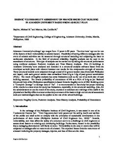
Damage Probability Matrices based on expert judgement and opinion were first introduced in ATC13 (ATC, 1985). More than 50 senior earthquake engineering experts were asked to provide low, best and high estimates of the damage factor (the ratio of loss to replacement cost, expressed as a percentage) for Modified Mercalli Intensities (MMI) from VI to XII for 36 different building classes. The low and high damage factor estimates provided by the experts were defined as the 90% probability bounds of a lognormal distribution, whilst the best estimate was taken as the median damage factor (Figure 2). Weighted means of the experts’ estimates, based on the experience and confidence levels of the experts for each building class, were included in the averaging process, as described in Appendix G of ATC-13 (ATC, 1985). A lognormal distribution was then used to calculate the probability of a central damage factor by finding the area below the curve within a given damage factor range. Thus, a DPM could be produced for each intensity level for each building class. Examples of the use of DPMs based on the ATC-13 approach for the assessment of risk and loss include the city of Basel (Fah et al., 2001), Bogotá (Cardona and Yamin, 1997) and New Madrid (Veneziano et al., 2002).

5%

5%

ML 4.00

Fig. 2

MB 10.60

MH 18.20

Example of a lognormal distribution of the estimated damage factor for a given intensity showing the mean low (ML), mean best (MB), and mean high (MH) estimates of the damage factor (adapted from McCormack and Rad (1997))


79

A macroseismic method has recently been proposed (Giovinazzi and Lagomarsino, 2001, 2004) that leads to the definition of damage probability functions based on the EMS-98 macroseismic scale (Grünthal, 1998). The EMS-98 scale defines qualitative descriptions of “Few”, “Many” and “Most” for five damage grades for the levels of intensity ranging from V to XII for six different classes of decreasing vulnerability (from A to F). Damage matrices containing a qualitative description of the proportion of buildings that belong to each damage grade for various levels of intensity are presented in Table 2 for vulnerability class C. Table 2: Example of a Damage Model for Vulnerability Class C as Presented in EMS-98 Damage Level Intensity

Damage Grade 1

2

3

4

5

V VI

Few

VII

Few

VIII

Many

IX X

Few Many

Few Many

Few

XI

Many

XII

Most

The problems related to the “incompleteness” of the matrices (i.e., the lack of information for all damage grades for a given level of intensity) and the “vagueness” of the matrices (i.e., they are described qualitatively) have been tackled by Giovinazzi and Lagomarsino (2004) by assuming a beta damage distribution and by applying Fuzzy Set Theory, respectively. The damage probability matrices produced for each vulnerability class have been related to the building stock through the use of an empirical vulnerability index which depends on the building typology, the characteristics of the building stock (e.g., number of floors, irregularity, etc.) and the regional construction practices. This macroseismic method has already been applied in the risk assessment of the cities, Faro (Oliveira et al., 2004), Lisbon (Oliveira et al., 2005), and Barcelona (Lantada et al., 2004). Following the introduction of DPMs based on intensity, the assessment of seismic risk on a large scale was made possible in both an efficient and cost-effective manner because in the past seismic hazard maps were also defined in terms of macroseismic intensity. The use of observed damage data to predict the future effects of earthquakes also has the advantage that when the damage probability matrices are applied to regions with similar characteristics, a realistic indication of the expected damage should result and many uncertainties are inherently accounted for. However, there are various disadvantages associated with the continued use of empirical methods such as DPM’s: • A macroseismic intensity scale is defined by considering the observed damage of the building stock and thus in a loss model both the ground motion input and the vulnerability are based on the observed damage due to earthquakes. • The derivation of empirical vulnerability functions requires the collection of post-earthquake building damage statistics at sites with similar ground conditions for a wide range of ground motions: this will often mean that the statistics from multiple earthquake events need to be combined. In addition, large magnitude earthquakes occur relatively infrequently near densely populated areas and so the data available tends to be clustered around the low damage/ground motion end of the matrix thus limiting the statistical validity of the high damage/ground motion end of the matrix. • The use of empirical vulnerability definitions in evaluating retrofit options or in accounting for construction changes (that take place after the earthquakes on which those are based) cannot be explicitly modelled; however simplifications are possible, such as upgrading the building stock to a lower vulnerability class.

80 •

•

Development of Seismic Vulnerability Assessment Methodologies over the Past 30 Years Seismic hazard maps are now defined in terms of PGA (or spectral ordinates) and thus PGA needs to be related to intensity; however, the uncertainty in this equation is frequently ignored. When the vulnerability is to be defined directly in terms of PGA, where recordings of the level of the ground shaking at the site of damage are not available, it might be necessary to predict the ground shaking at the site using a ground motion prediction equation; however, again the uncertainty in this equation needs to be accounted for in some way, especially the component related to spatial variability. When PGA is used in the derivation of empirically-defined vulnerability, the relationship between the frequency content of the ground motions and the period of vibration of the buildings is not taken into account.

2. Vulnerability Index Method The “Vulnerability Index Method” (Benedetti and Petrini, 1984; GNDT, 1993) has been used extensively in Italy in the past few decades and is based on a large amount of damage survey data; this method is ‘indirect’ because a relationship between the seismic action and the response is established through a ‘vulnerability index’. The method uses a field survey form to collect information on the important parameters of the building which could influence its vulnerability: for example, plan and elevation configuration, type of foundation, structural and non-structural elements, state of conservation and type and quality of materials. There are eleven parameters in total, which are each identified as having one of four qualification coefficients, K i , in accordance with the quality conditions – from A (optimal) to D (unfavourable) – and are weighted to account for their relative importance. The global vulnerability index of each building is then evaluated using the following formula: 11

I v = ∑ K iWi

(1)

i =1

The vulnerability index ranges from 0 to 382.5, but is generally normalised from 0 to 100, where 0 represents the least vulnerable buildings and 100 the most vulnerable. The data from past earthquakes is used to calibrate vulnerability functions to relate the vulnerability index ( I v ) to a global damage factor

(d ) of buildings with the same typology, for the same macroseismic intensity or PGA. The damage factor ranges between 0 and 1 and defines the ratio of repair cost to replacement cost. The damage factor is assumed negligible for PGA values less than a given threshold and it increases linearly up until a collapse PGA, from where it takes a value of 1 (Figure 3). 1

Damage factor, d

Iv = 80

60

40

20

10

5

0.8 0.6 0.4 0.2 0 0

0.2

0.4

0.6

0.8

1

PGA

Fig. 3

Vulnerability functions to relate damage factor (d ) and peak ground acceleration (PGA) for different values of vulnerability index ( I v ) (adapted from Guagenti and Petrini (1989))

RISK_UE (An Advanced Approach to Earthquake Risk Scenarios with Application to Different European Towns) was a major research project financed by the European Commission (see www.riskue.net). Seven European cities (Barcelona, Bitola, Bucharest, Catania, Nice, Sofia and Thessaloniki) were


81

involved in this project, whose main objective was to develop a general methodology for the seismic risk assessment of European towns. The Vulnerability Index Method was adopted as one of the vulnerability assessment procedures which were developed and successfully applied to all of the aforementioned cities. The “Catania Project”, discussed in Faccioli et al. (1999) and GNDT (2000), used an adapted vulnerability index method for the risk assessment of both masonry and reinforced concrete buildings. Some modifications to the original vulnerability index procedure were applied in that a rapid screening approach was used to define the vulnerability scores of the buildings, following the guidelines of ATC-21 (ATC, 1988). As in the original procedure, the vulnerability score was obtained from the weighted sum of eleven parameters; however, only some were directly obtained from a field assessment, while the rest were based on a range of values according to historic or recent construction practices within the region, thus leading to a lower and an upper bound to I v for each building. Vulnerability functions for old masonry buildings were calibrated to the damage observed after the 1976 Friuli and the 1984 Abruzzo earthquakes, and damage and peak ground acceleration were correlated through the relationship proposed by Guagenti and Petrini (1989) (see Figure 3). The main advantage of ‘indirect’ vulnerability index methods is that they allow the vulnerability characteristics of the building stock under consideration to be determined, rather than base the vulnerability definition on the typology alone. Nevertheless, the methodology still requires expert judgement to be applied in assessing the buildings, and the coefficients and weights applied in the calculation of the index have a degree of uncertainty that is not generally accounted for. Furthermore, in order for the vulnerability assessment of buildings on a large (e.g., national) scale to be carried out using vulnerability indices, a large number of buildings which are assumed to represent the national building stock need to be assessed and combined with the census data (e.g., Bernardini, 2000); in a country where such data is not already available, the calculation of the vulnerability index for a large building stock would be very time consuming. However, in any risk or loss assessment model a detailed collection of input data is required for application at the national scale. 3. Continuous Vulnerability Curves Continuous vulnerability functions based directly on the damage of buildings from past earthquakes were introduced slightly later than DPMs; one obstacle to their derivation being the fact that macroseismic intensity is not a continuous variable. This problem was overcome by Spence et al. (1992) through the use of their Parameterless Scale of Intensity (PSI) to derive vulnerability functions based on the observed damage of buildings using the MSK damage scale (Figure 4). Orsini (1999) also used the PSI ground-motion parameter to derive vulnerability curves for apartment units in Italy. Both studies subsequently converted the PSI to PGA using empirical correlation functions, such that the input and the response were not defined using the same parameter. Sabetta et al. (1998) used post-earthquake surveys of approximately 50000 buildings damaged by destructive Italian earthquakes in order to derive vulnerability curves. The database was sorted into three structural classes and six damage levels according to the MSK macroseismic scale. A mean damage index, calculated as the weighted average of the frequencies of each damage level, was derived for each municipality where damage occurred and each structural class. Empirical fragility curves with a binomial distribution were derived as a function of PGA, Arias Intensity and effective peak acceleration. Rota et al. (2006) have also used data obtained from post-earthquake damage surveys carried out in various municipalities over the past 30 years in Italy in order to derive typological fragility curves for typical building classes (e.g., seismically designed reinforced concrete buildings of 1-3 storeys). Observational damage probability matrices were first produced and then processed to obtain lognormal fragility curves relating the probability of reaching or exceeding a given damage state to the mean peak ground acceleration at the coordinate of the municipality where the damaged buildings were located. The PGA has been derived using the magnitude of the event and the distance to the site based on the attenuation relation by Sabetta and Pugliese (1987), assuming rock site conditions. Alternative empirical vulnerability functions have also been proposed, generally with normal or lognormal distributions, which do not use macroseismic intensity or PGA to characterise the ground motion but are related to the spectral acceleration or spectral displacement at the fundamental elastic period of vibration (e.g., Rossetto and Elnashai, 2003; Scawthorn et al., 1981; Shinozuka et al., 1997). The latter has been an important development as it has meant that the relationship between the frequency content of the ground motion and the fundamental period of vibration of the building stock is taken into

82


consideration; in general this has been found to produce vulnerability curves which show improved correlation between the ground motion input and damage (see Figure 5). 1.0

P(d >D / PSI)

0.8

0.6

0.4

D1 D2 D3 D4 D5

0.2

0.0 0

5

10

15

20

PSI

Fig. 4

Vulnerability curves produced by Spence et al. (1992) for bare moment-resisting frames using the parameterless scale of intensity (PSI); D1 to D5 relate to damage states in the MSK scale

Fig. 5

Example of the difference in the vulnerability point distribution using the observations of low and mid-rise building damages after the 1995 Aegion (Greece) earthquake for different ground motion parameters: (a) PGA, and (b) Spectral displacement at the elastic fundamental period (Rossetto and Elnashai, 2003)

The introduction of vulnerability curves based on spectral ordinates, rather than PGA or macroseismic intensities, has also certainly been facilitated by the emergence of more and more attenuation equations in terms of spectral ordinates. 4. Screening Methods In Japan, the evaluation of the seismic performance of existing reinforced concrete buildings with less than 6 storeys has been carried out since 1975 with the use of the Japanese Seismic Index Method (JBDPA, 1990). Three seismic screening procedures are available to estimate the seismic performance of a building with the reliability increasing with each screening level. The seismic performance of the building is represented by a seismic performance index, I S , which should be calculated for each storey in every frame direction within the building using the following equation:


83

I S = Eo S DT

(2)

where E o is for the basic structural performance, S D is the sub-index concerning the structural design of the building, and T is the sub-index for the time-dependent deterioration of the building. The method to calculate E o involves the calculation and multiplication of an ultimate strength index C and a ductility index F , considering the failure mode, the total number of storeys and the position of the storey under examination. The influence of irregularity, stiffness and/or mass concentration of a structure on the seismic performance should be accounted for by the sub-index S D . The influence of deterioration and cracking is taken into account by the sub-index T , which is based on the data found through a field investigation. Once the seismic performance index I S has been calculated it should be compared with the seismic judgement index for the structure I S 0 to determine whether the building can be called “safe” against an assumed earthquake ground motion (i.e., if I S > I S 0 ). There are three possibilities depending on the difference between I S and I S 0 : •

I S ≥ I S 0 ; corresponds to a low vulnerability condition for all three screening levels,

•

I S