(DOI): 10.5935/PAeT.V6.N3.01 This article is presented in English with abstracts in Spanish and Portuguese Brazilian Journal of Applied Technology for Agricultural Science, Guarapuava-PR, v.6, n.3, p.07-16, 2013
Cientific Paper
Abstract
Development of technologies and methods for monitoring the spatial variability of air temperature in greenhouse environment
Climatic factors directly influence growth and productivity of plants inside greenhouses, where temperature can be considered one of the major parameter in this context. Thus, the aim of this research was to develop a low cost device Diego Scacalossi Voltan1 for thermal sensing and data acquisition, and use it in data collection and analysis of spatial variability of temperature Rogério Zanarde Barbosa1 inside a greenhouse with tropical climate. The developed João Eduardo Machado Perea Martins2 equipment for thermal measurements showed a high degree Célia Regina Lopes Zimback3 of accuracy and fast responses in measurements, proving its efficiency. The data analysis interpretations were made from the elaborations of variograms and of tridimensional maps generated by a geostatistical software. The processed data analysis presented that a greenhouse without thermal control has spatial variations of air temperature, both in the sampled horizontals layers as in the three analyzed vertical columns, presenting variations of up to 3.6 ºC in certain times.
Keywords: Spatial dependence; geostatistics; thermometric tool.
Desenvolvimento de tecnologias e métodos para monitoramento da variabilidade espacial da temperatura em ambientes de cultivo protegido
Resumo Os fatores climáticos influenciam diretamente o crescimento das plantas e a produtividade dentro de casas de vegetação, sendo que a temperatura pode ser considerada um dos fatores mais importantes nesse contexto. Assim, o objetivo desse trabalho foi desenvolver um dispositivo de baixo custo para sensoriamento térmico e aquisição de dados, e utilizá-lo no levantamento de dados e análise da variabilidade espacial da temperatura no interior de uma casa de vegetação de clima tropical. O dispositivo físico de medição térmica desenvolvido apresentou um alto grau de exatidão e respostas imediatas nas medições, comprovando sua eficiência. As interpretações dos dados foram feitas a partir da elaboração de variogramas e de mapas tridimensionais gerados por um software geoestatístico. Os dados analisados mostraram que uma casa de vegetação sem controle térmico apresenta variações espaciais da temperatura do ar tanto nas camadas horizontais amostradas, como nas três alturas de colunas verticais analisadas, apresentando variações de até 3,6ºC em determinados horários.
Palavras-chave: Dependência espacial; geoestatística; ferramenta termométrica.
Desarrollo de tecnologías y métodos para monitoreo de la variabilidad espacial de la temperatura en ambientes de cultivo protegido
Resumen Los factores climáticos influyen directamente en el crecimiento de las plantas y la productividad en los invernaderos, siendo que la temperatura puede ser considerad como uno de los factores más importantes en este contexto. El objetivo de este trabajo fue desarrollar un dispositivo de bajo costo para el sensoriamento térmico y adquisición de datos, y su utilización en la recolección de datos y análisis de la variabilidad espacial de la temperatura dentro de un invernadero con clima tropical. El dispositivo físico de medición térmica desarrollado mostró un alto grado de precisión y respuestas inmediatas en las Received at: 09/04/2013
Accepted for publication at: 09/09/2013
1 Post Graduation student Agronomy - Irrigation and drainage. Universidade Estadual Paulista "Júlio de Mesquita Filho" (UNESP) Faculdade de Ciências Agronômicas. Botucatu-SP. E-mail:
[email protected];
[email protected] 2 Dr. Prof. Departamento de Computação (FC). Universidade Estadual Paulista "Júlio de Mesquita Filho" (UNESP) - Faculdade de Ciências Agronômicas. Botucatu-SP. E-mail:
[email protected] 3 Dra. Prof. Departamento de Recursos Naturais. Universidade Estadual Paulista "Júlio de Mesquita Filho" (UNESP) - Faculdade de Ciências Agronômicas. Botucatu-SP. E-mail:
[email protected]
Applied Research & Agrotecnology v6 n3 sept/dec. (2013) Print-ISSN 1983-6325
(On line) e-ISSN 1984-7548
7
Voltan et al. (2013) mediciones, lo que demuestra su eficiencia. Las interpretaciones de los datos se hicieron con el desarrollo de variogramas y mapas tridimensionales generadas por un software geoestadístico. Los datos analizados mostraron que un invernadero sin control térmico presenta variaciones espaciales de la temperatura del aire, tanto en las capas horizontales muestreadas, como en las tres alturas de columnas verticales analizadas, mostrando variaciones de hasta 3,6 ºC en ciertos momentos.
Palabras clave: dependencia espacial; geoestadística; herramienta termométrica.
Introduction
the use of geostatistical methods appears as an efficient tool for the description and analysis of the spatial distribution of the temperature in greenhouses (SAPOUNAS et al., 2008). Although there are many commercial models of dispositive for thermal measurement, in this study we present the development of one of thermal sensing. Thus, the study has as objective to present an analysis of the spatial dependence of air temperature inside greenhouses using a measurement instrument developed for acquisition of temperature data.
The temperature is one of the most important factors to be observed in the agriculture (TERUEL, 2010; CHEN et al., 2011), since this parameter greatly influences the metabolic functions of the plants and even of animals (SOTO-ZARAZÚA et al., 2011). In greenhouse environments, AGUIAR et al. (2000), BÖHMER et al. (2008), ROMANINI et al. (2010) and ANDRADE et al. (2011) proved that the influence of the type of cover of greenhouse alter the internal temperature of these environments, showing that this factor must be taken into account for substantially affecting the yield. According to ZHANG et al. (2010), the thermal variation inside protected environments is related to many other factors, among them the solar radiation, convection movement of air masses in the greenhouse edges and by the dynamics of pressure of air steam which occurs due to a difference of internal and external temperature of the greenhouse. The advanced control of climate in a greenhouse involves many variables and complicated non linear processes, which can demand a high financial investment and a great technological effort to achieved efficient and reliable results (KITTAS and BARTZANAS, 2007; ÖDUK and ALLAHVERDY, 2011; XIU-HUA and LEI, 2011). Many researchers simplify the study, understanding the interior climate of the greenhouse as uniform (KITTAS and BARTZANAS, 2007; KOLOKOTSA et al., 2010) and thus, usually perform the climatic monitoring through measurements in a unique spot, such as the center of the greenhouse, and the information are then extrapolated for the other spots. This technique is simple for the fact of demanding the physical measurement of only a specific spot. However, HASAN et al. (2009) and JÁNOS et al. (2010) show that, in the specific case of the temperature, the creation of a process for measurement in many spots of the greenhouse allows the making of a map. Inside this concept of measurements in several places and maps creation,
Material and Methods The development of the low cost dispositive for thermal sensing was based in the temperature sensor LM35, which can be found in the Brazilian market, with cost below to R$ 10.00, it also has a high degree of reliability, with linear output of voltage 10 mV/°C, accuracy of 0.5 °C, power ranging from 4 to 30 V, electric current consumption of 60 µA and auto heating inferior to 0.1 °C. The output voltage can be directly read on a multimeter adjusted in a scale of millivolts, presenting a relation with the measured temperature in degrees centigrade (Temp) expressed by Temp = Volt/10. The methodology of development of the analysis of spatial thermal variability, where the geostatistics is used as a tool allows quantifying the spatial dependence between the sampled variables and reproduce in graphics how it behaves on the environment. Thus, in this study the measures of temperature were sampled in different spots inside a greenhouse located in the Universidade Estadual Paulista, Faculty of Agronomic Sciences, in Botucatu SP, with geographical coordinates of 22°51’3’’ of south latitude and 48°25’37” of longitude west and 786 m of altitude. The representative spots for each air volume were pre established in the plating lines of the greenhouse, grid shaped (sampling grid), defined in 0.8 m between lines and 1.0 m between spots, distributed in 19 spots for each one of the six cultivations lines, totalizing 114 spots. In October
Applied Research & Agrotecnology Print-ISSN 1983-6325
8
v6 n3 sept/dec. (2013)
(On line) e-ISSN 1984-7548
Development of technologies and methods… Desenvolvimento de tecnologias e métodos… Desarrollo de tecnologías y métodos… 8th of 2010 for each of the 114 spots were performed measurements in three different heights, which were 0.30, 1.20 and 2.00 m. This experiment was done three times a day, at 9, 12 and 16 hours, so that was established a spatial analysis associated to temporal variations. The temperature was sequentially measured in each spot, being that the time of the total route was 10 min for the measure in each one of the three heights. The greenhouse used in this study was of the arch type, 6 m wide, 24 m of length and a ceiling height of 3 m, positioned in the East-West. The lateral windows were coated with a polyethylene mesh of anti-aphid protection. In the superior edges, longitudinal direction, the greenhouse has two frontal windows with controlled opening to allow ventilation in the warmest times of the day. It also has a polyethylene cover of low density for protection against rain, from the ridge to the eaves. The values calculated from the 114 sampled spots to obtain the descriptive statistic were relevant to verify the variability of the air temperature data. It were calculated the average, median, maximum and minimum value, amplitude, standard deviation and coefficient of variation (CV). The function of spatial variance γ (h), known as variogram allowed to calculate the spatial dependence by the variance measure of the differences of the sampled values which are distant in h m. It is expressed by: 1 N (h ) 2 ∑ [Z ( xi ) − Z (xi + h )] 2 N (h ) i =1
γ (h ) =
0.25 and 0.75 it is moderate spatial dependence; and values of ≤ 0.25 as low spatial dependence. After the analysis of spatial dependence, the data were interpolated by the kriging method. This method allows estimating values of variables distributed in the space using the structural properties of the variogram. The results of the interpolation were visualized in tridimensional maps representing the spatial distributions of air temperature. All the data obtained for the analysis were calculated using the program GS+ (Geostatistical for Environmental Sciences) (Robertson 1998).
Results and Discussion This section presents the obtained results, being that, for effects of organization they were divided in two parts which have the discussions related to the low cost dispositive for thermal sensing and the analysis on the thermal spatial variability. Low cost dispositive for thermal sensing Figure 1 exemplifies the electronic circuit and the physical assembling of the dispositive developed in this study, whose mounting is simple and has the advantage of allowing that the height of the positions of temperature measurement gets easier and quickly altered. In this study, the dispositive of thermal sensing includes, besides the LM35 sensor, mechanical parts of the probe, the meter for visualization of the measurements and a box of battery conditioning. The probe was installed in an aluminum tube with 100 cm, being longer than the usual to allow the easy measurement in different heights and to enable its insertion in closed places. In one tip was placed a LM35 fixed in epoxy resin and in the other edge was placed a manual support and a small plastic box for conditioning of a battery of 9V used to power the sensor. The output of the voltage (Volt) was directly read by a simple multimeter DT830D model and its display had 3 ½ digits. Thus, in measurement scale of voltage of 2,000 mV, the temperature can be directly calculated with up to two digits integer and a decimal, which is fairly suitable for numerous agricultural applications. Initially was tested a circuit with this physical assembling and without special precautions with the connection of grounding or shielding. For analysis of performance of the developed thermometer were made 10 operational tests, being that in each test were performed 600 temperature measurements, using an
[1]
Where: N(h) is the number of pairs of median values Z(si), Z(si+h), separated by a vector h, being h the distance between the spots of all the sampled values. The calculated values for the elaboration of the semivariograms were: nugget effect or ‘Nugget’ (Co), which represents the value of γ h) when h ( = 0; Sill (Co + C) is when the value of γ (h) stabilizers and its value is approximately equal to the data variance; the Range (a) is the distance h when γ (h) achieves the level and the samples become independent. These parameters assist in the analysis of spatial dependence calculated by the relation C/Co + C, denominated structure or spatial proportion which, according to the classification adapted by ZIMBACK (2001), if the obtained value of this ratio is ≥ 0.75, it is classified as strong spatial dependence; between
Applied Research & Agrotecnology v6 n3 sept/dec. (2013) Print-ISSN 1983-6325
(On line) e-ISSN 1984-7548
p. 07-16
9
Voltan et al. (2013)
Figure 1. Electronic circuit of the thermometer with the LM35 sensor (left) and the actual photograph of the developed thermometer (right). interval of 10 ms between each measurement. Figure 2 shows the graphic of voltage variation of output of the developed thermometer for the first sampling done. Table 1 shows the obtained results in the ten samplings, where it can be verified that the values of the averages and of standard deviation of sampling are very close, proving the stability of the system. In the table, the value of each sample average is represented in the form of voltage, which can be directly converted in temperature. Table 1 data allows to calculate the average of the output voltage means in 269.7 mV, with a standard deviation of 0.264 and with a coefficient of variation of 0.098% and first
confidence interval between 269.436 and 269.964 mV. With basis in this data, it can be concluded that the developed dispositive of electronic thermal sensing in this study showed a low cost and excellent accuracy in the measurements, achieving the initial objective for its development. Analysis of the spatial thermal variability Figure 3 shows the temperature variation and solar radiation in the external part and close to the greenhouse at the day of the measurements, allowing that the internal data were also analyzed in
Figure 2. Variation of the output voltage, in volts, of the developed thermometer. Applied Research & Agrotecnology Print-ISSN 1983-6325
10
v6 n3 sept/dec. (2013)
(On line) e-ISSN 1984-7548
Development of technologies and methods… Desenvolvimento de tecnologias e métodos… Desarrollo de tecnologías y métodos… comparison with external factors, The air temperature presented variations between 17.62 and 28.19 °C during the day, with an average of 24.81 °C, and solar radiation with values between 852 to 1,029 W/m². Table 2 shows the statistical variables calculated through the data registered in the measurement done at the three schedules and three heights of the operation. It can be observed that to the schedules 9h and 16h the coefficients of variation of the temperature averages in the three different heights was always inferior to 1.8%, however at 12h was critical, being that the temperature within the greenhouse presented peak values with a difference of 3.6 °C at a height of 0.30 m. Tables 3, 4 and 5 show, respectively, the variogram parameters obtained through the geostatic analysis, adjusted by the software GS+ for the data
p. 07-16
of the measures at 9, 12 and 16 h, considering the higher value of regression R². The values assisted in the elaboration of the variograms and, for it, were calculated the values of the Nugget effect (C0), of the Sill (C + C0), of Range (a), of regression (R²) and of the structure or spatial proportion [C/ (C0 + C)]. Thus, they were used to calculate the experimental variograms and then adjust them to the theoretical models showed in the figures 4, 5 and 6. At the three schedules, except for the heights 0.30 and 1.20 m at 9h and 1.20 m at 16h, all variograms were adjusted by the Gaussian model. This model reveals that the temperatures of the sampled spots presented continuity among them with certain regularity. The Gaussian model adjusts to the spots not going through them all and smoothes the curve when approaching to zero. This model is also used
Table 1. Statistical values of 10 samplings, with 600 samples each, of the output voltage signal of the thermometer developed with the LM35. Sampling 1 2 3 4 5 6 7 8 9 10
Sample Average (milivolts) 269.039 269.462 269.571 269.654 269.744 269.737 269.744 269.747 269.941 269.961
Standard Deviation 0.931 0.944 0.910 0.894 0.902 0.943 0.920 0.937 0.883 0.921
Coefficient of variation (%) 0.346 0.350 0.337 0.331 0.334 0.349 0.341 0.347 0.327 0.341
Figure 3. Behavior of the air temperature and of the solar radiation in the external environment in relation to the greenhouse, in the intervals in which was measured the internal air temperature of the same. Applied Research & Agrotecnology v6 n3 sept/dec. (2013) Print-ISSN 1983-6325
(On line) e-ISSN 1984-7548
11
Voltan et al. (2013) Table 2. Results of the descriptive analysis of statistics of the values collected of air temperature at the schedules 9, 12 and 16h at the heights of 0.30, 1.20 and 2.00 m. Descriptive statistics
9 hours
12 hours
16 hours
0.30 (m) 24.02 24.10 24.70 23.00 1.70
1.20 (m) 25.28 25.20 26.50 24.70 1.80
2.00 (m) 25.55 25.55 26.40 24.60 1.80
0.30 (m) 28.87 28.80 30.60 27.00 3.60
1.20 (m) 28.91 29.00 30.00 27.80 2.20
2.00 (m) 30.62 30.50 32.20 29.10 3.10
0.30 (m) 28.26 28.20 29.50 27.50 2.00
1.20 (m) 31.38 31.50 31.90 30.60 1.30
2.00 (m) 30.06 29.90 31.60 28.90 2.70
Standard deviation
0.3865
0.3885
0.4516
0.9619
0.5959
1.0351
0.3615
0.3139
0.4893
CV (%)
1.61
1.54
1.77
3.33
2.06
3.38
1.28
1.00
1.63
Average Median Maximum Minimum Total range
Table 3. Variogram parameters set at the time of 9h. Height (m) 0.30 1.20 2.00
Variogram model Exponential Exponential Gaussian
Nugget variance (Co) 0.0686 0.0502 0.0276
Sill (Co+C)
Range (m)
R2
C/Co+C
0.3242 0.3494 0.2302
62.97 62.97 5.5252
0.702 0.930 0.919
0.788 0.730 0.880
Table 4. Variogram parameters set at the time of 12h. Height (m) 0.30 1.20 2.00
Variogram model Gaussian Gaussian Gaussian
Nugget variance (Co) 0.0010 0.0010 0.0010
Sill (Co+C)
Range (m)
R2
C/Co+C
0.9610 0.3470 1.2760
2.4942 2.4595 4.5207
0.860 0.909 0.896
0.9990 0.9970 0.9990
Table 5. Variogram parameters set at the time of 16h. Height (m) 0.30 1.20 2.00
Variogram model Gaussian Spherical Gaussian
Nugget variance (Co) 0.0230 0.0176 0.0016
Sill (Co+C)
Range (m)
R2
C/Co+C
0.1220 0.1142 0.2842
4.9017 5.4700 5.1442
0.952 0.797 0.874
0.811 0.846 0.994
to represent extremely continuous variables and the value of the Range is correspondent to 95% of the Sill (Isaaks and Srivastava 1989). In figure 4 (A) and (B) the exponential model was better adjusted to the heights 0.30 and 1.20 m at 9h. This model is evident due to the Sill tends to the infinite, or better, the variance curve is highly dispersed in relation to the distance between samples. Despite the elaborated variogram range for the
height 1.20 at 16h being close to the other variograms adjusted to the Gaussian model, it presented a linear behavior and with a rapid growth in the source, characteristic of the spherical model, as presented in figure 6 (B). From the determination of the variogram parameters was assessed the Range of the samples, parameter which represents the maximum distance that the spots are related spatially to the same
Applied Research & Agrotecnology Print-ISSN 1983-6325
12
v6 n3 sept/dec. (2013)
(On line) e-ISSN 1984-7548
Development of technologies and methods… Desenvolvimento de tecnologias e métodos… Desarrollo de tecnologías y métodos…
p. 07-16
Figure 4. Theoretical models of the variograms adjusted for the 9h schedule, at the heights 0.30, 1.20 and 2.00 m. (A) Exponential, (B) Exponential and (C) Gaussian.
Figure 5. Theoretical models of the variograms adjusted for the 12h schedule, at the heights 0.30, 1.20 and 2.00 m. (A) Gaussian, (B) Gaussian and (C) Gaussian.
Figure 6. Theoretical models of the variograms adjusted for the 16h schedule, at the heights 0.30, 1.20 and 2.00 m. (A) Gaussian, (B) Spherical and (C) Gaussian. variable and which, according to ANDRADE (2002), marks the distance from which the samples become independents. At the 9h schedule, the Range value for the heights 0.30 and 1.20 was 62.97 m. This distance reveals that the air temperature is presenting very close values and the variable starts to be independent starting from this distance. This shows that, possibly, due to the non direct incidence of solar rays in the respective heights at this time, in the west part
of the structure, the environment is not suffering direct interference of solar radiation, characterizing a homogeneous environment in relation to the air temperature. At 2.00 m of height, the solar rays were reflecting on the greenhouse cover and the top of the plants and the Range distance of air temperature at this height drastically fell to 5.52m, as presented in Table 2. During the warmest moment of the day, registered at 12h, the Range achieved the smallest
Applied Research & Agrotecnology v6 n3 sept/dec. (2013) Print-ISSN 1983-6325
(On line) e-ISSN 1984-7548
13
Voltan et al. (2013) values on the three sampled categories (0.30, 1.20 and 2.00 m of height) which were 2.49, 2.45 and 4.52 m, respectively. This schedule presented the most significant temperature variations in relation to the 9 and 16h schedules, and possibly its range was smaller due to the influence of the phenomenon which occurred in isolation inside the greenhouse due to the high reflection of solar radiation. Still at 12h, in figure 8 is observed that the highest air temperatures occupy the central region of the greenhouse, this variation can be a consequence of the opened lateral of the structure, thus contributing to the dissipation of heat during the moment that the solar radiation is more intense. At 16h, the Range values for the 0.30, 1.20 and 2.00 m heights were respectively 4.90, 5.47 and 5.14 m. There was a slight increase of the Range in comparison to the 12h schedule. It can be observed in figure 1 that the air temperature in the greenhouse exterior is decreasing, due to the smaller influence of the solar radiation, and the temperature of the internal air volumes in the greenhouse tends to homogenize, possibly exchanging heat. FURLAN and FOLEGATTI (2002), assessing the air temperature distribution in controlled environment observed that even after the completion of nebulization, at 17h, the heat transmission from the plastic cover to the internal environment was very low. It can be seen
in table 2 that the total amplitude decreases 0.4, 0.9 and 1.6 ºC in relation to the 12h schedule for the heights of 0.30, 1.20 and 2.00 m. In this sense, the variograms analysis showed that there was spatial dependence for all times and heights, as shown in the figures 4, 5, 6. It is observed that, according with the index of spatial dependence adapted by ZIMBACK (2001), except for the assessment of 9h at the height 1.20 m which presented moderate spatial dependence, all other values had strong spatial dependence. The visualization of the spatial dependence was observed in maps generated by the software GS+ with 3D representation of the spatial distribution of temperature of the sampled spots at 9, 12 and 16h, obtained through interpolation of the data by kriging. Figures 7, 8 and 9 show the graphics of spatial distribution of temperature for each studied schedule at 0.30, 1.20 and 2.00 m of height. The current study demanded the temperature measurement in several spots of the greenhouse. Thus, for costs reduction it was used only one datalogger and one probe, with only one sensor. Due to the work conditions, another possibility is to use a single meter with various sampling points in the same set. Being these possibilities a motivation for new researches.
Figure 7. 3D Representation of the spatial distribution of air temperature at 9:00h at 0.30 m, 1.20 m and 2.00 m.
Figure 8. 3D Representation of the spatial distribution of air temperature at 12:00h at 0.30 m, 1.20 m and 2.00 m. Applied Research & Agrotecnology Print-ISSN 1983-6325
14
v6 n3 sept/dec. (2013)
(On line) e-ISSN 1984-7548
Development of technologies and methods… Desenvolvimento de tecnologias e métodos… Desarrollo de tecnologías y métodos…
p. 07-16
Figure 9. 3D Representation of the spatial distribution of air temperature at 16:00h at 0.30 m, 1.20 m and 2.00 m.
Conclusions
analysis of temperature variation in greenhouses. The developed electronic thermometer, besides of the low cost and simplicity of assembling, presented a high accuracy, being considerate satisfactory, which ensures reliability in the thermal measurements done with the same. The detected variations can influence in the uniformity development and in the crops yield, besides of assisting in strategic measures of climatic control, facilitating the management and decision taking.
The air temperature in greenhouse presented strong spatial dependence for all assessed times and heights, except at 9h and 1.20 of height, which presented moderate spatial dependence. The air temperature variations within the greenhouse had maximum amplitude of 3.6 °C at 12h and minimum amplitude of 1.3 °C at 16h. The technological resources can be used in a cheap and efficient from for the monitoring and
References ANDRADE, A. R. S. Aplicação da Teoria fractal e da geoestatística na estimativa da condutividade hidráulica saturada e do espaçamento entre drenos. Botucatu/SP, Tese (Doutorado em Agronomia) - Faculdade de Ciências Agronômicas, Universidade Estadual Paulista, Botucatu, 2002. 181f. ANDRADE, J.W. S.; FARIAS JUNIOR, M.; SOUSA, M.A.; ROCHA, A.C. Utilização de diferentes filmes plásticos como cobertura de abrigos. Acta Scientiarum. Agronomy. v.33, n.3, p.437-443, 2011. BÖHMER, C.R.K.; MAUCH, C.R.; ASSIS, S.V.; SCHÖFFEL, E.R.; MENDEZ, M.E.G. Alterações na temperatura do ar proporcionadas por estufa de polietileno, durante um cultivo de feijão-vagem. Revista Brasileira de Agrometeorologia, v.16, n.2, p.143- 148, Ago., 2008. BOJACÁ, C. R., GIL, R., COOMAN, A. Use of geostatistical and crop growth modelling to assess the variability of greenhouse tomato yield caused by spatial temperature variations. Computers and Electronics in Agriculture, v.65, n.2, p.219-227, 2009. BRITO, A.A.A. Casa de vegetação com diferentes coberturas: Desempenho em condição de verão. Tese de Doutorado (Pós-graduação em Engenharia Agrícola), UFV, Viçosa, 2000. 100p. CHEN, C.; SHEN, T.; WENG, Y. Simple model to study the effect of temperature on the greenhouse with shading nets. African Journal of Biotechnology, v.10, n.25, p.5001-5014, 2011. DJEVIC, M.; DIMITRIJEVIC, A. Energy consumption for different greenhouse constructions. Energy, v.34, n.9, p.1325-1331, 2009. EVANGELISTA, A.W.P.; PEREIRA, G.M. Efeito da cobertura plástica de casa-de-vegetação sobre os elementos meteorológicos em lavras, M.G. Ciência e Agrotecnologia, v.25, n.4, p.952-957, 2001. FURLAN, R.A.; FOLEGATTI, M.V. Distribuição vertical e horizontal de temperaturas do ar em ambientes protegidos. Revista Brasileira de Engenharia Agrícola e Ambiental,, v.6, n.1, p.93-100, 2002. Applied Research & Agrotecnology v6 n3 sept/dec. (2013) Print-ISSN 1983-6325
(On line) e-ISSN 1984-7548
15
Voltan et al. (2013) HASAN, O.; ATILGAN, A.; BUYUKTAS, K.; ALAGOZ, T. The efficiency of fan-pad cooling system in greenhouse and building up of internal greenhouse temperature map. African Journal of Biotechnology, v.8, n.20, p.5436-5444, 2009. ISAAKS, E.H.; SRIVASTAVA, R.M. An introduction to applied geostatistics. New York: Oxford University Press, 1989. 560p. JÁNOS, S.; MARTINOVIĆ, G.; MATIJEVICS, I. WSN implementation in the greenhouse environment using mobile measuring station. International Journal of Electrical and Computer Engineering Systems, v.1, n.1, p.37-44,, 2010. KITTAS, C.; BARTZANAS, T. Greenhouse microclimate and dehumidification effectiveness under different ventilator configurations. Journal Building and Environment, v.42, n.10, p.3774-3784, 2007. KOLOKOTSA, D.; SARIDAKIS, G.; DALAMAGKIDIS, K.; DOLIANITIS, S.; KALIAKATSOS, I. Development of an intelligent indoor environment and energy management system for greenhouses. Journal Energy Conversion and Management, v.51, n.1, p.155-168, Jan., 2010. MESMOUDI, K.; SOUDANI, A.; BOURNET, P.E. The determination of the inside air temperature of a greenhouse with tomato crop, under hot and arid climates. Journal of Applied Science in Environmental Sanitation, v.5, n.2, p.117-129, 2010. ÖDUK, M. N.; ALLAHVERDY, N. The advantages of fuzzy control over traditional control system in greenhouse automation. In. anais Artificial Intelligence & Machine Learning Conference. Dubai: UAE, 2011. p.91-97. SAPOUNAS, AA., NIKITA-MARTZOPOULOU, CH. and SPIRIDIS, A. Prediction the spatial air temperature distribution of an experimental greenhouse using geostatistical methods. In anais: International Symposium on High Technology for Greenhouse System Management: Greensys200, Acta Horticulturae, Naples, v.2, n.801, p.495-500, 2008. SILVA, M.A.A.E.; GALVANI, E. ; ESCOBEDO, J.F.; CUNHA, AR. Avaliação da temperatura e umidade relativa do ar em estufa com cobertura de polietileno. In. anais Congresso Brasileiro de Meteorologia, 11, Rio de Janeiro, RJ: Sociedade Brasileira de Meteorologia, 2000. 1 CD-ROM. SONI, P.; SALOKHE, V.M.; TANTAU, H.J. Effect of Screen Mesh Size on Vertical Temperature Distribution in Naturally Ventilated Tropical Greenhouses. Biosystems Engineering, v. 92, n. 4, p. 469–482, 2005. SOTO-ZARAZÚA, G.M.; GARCIA, E.R.; AYALA, M.T. Temperature effect on fish culture tank facilities inside greenhouse. International Journal of the Physical Sciences, v.6, n.5, p.1039-1044, 2011. TERUEL, B.J. Controle automatizado de casas de vegetação: variáveis climáticas e fertirrigação. Revista Brasileira de Engenharia Agrícola e Ambiental, v.14, n.3, p.237-245, 2010. WARRICK, A.W.; NIELSEN, D.R. Spatial variability of soil physical properties in the field. In: HILLEL, D. (Ed.). Application of soil physics. New York: Academic Press, 1980. 385p. XIU-HUA, W.; LEI, Z. Simulation on temperature and humility nonlinear controller of greenhouses. In. anais International Conference on Intelligent Computation Technology and Automation (ICICTA), Shenzhen: 2011, p.500-503. ZHANG, Z. K.; LIU, S. H.; HUANG, Z. J. Estimation of cucumber evapotranspiration in solar greenhouse in northeast China. Agricultural Sciences in China, v.9, n.4, p.512-518, 2010. ZIMBACK, C.R.L. Análise espacial de atributos químicos de solos para fins de mapeamento da fertilidade. Tese de Livre-Docência (Livre-Docência em Levantamento do solo e fotopedologia), FCA/UNESP, 2001. 114 p.
Applied Research & Agrotecnology Print-ISSN 1983-6325
16
v6 n3 sept/dec. (2013)
(On line) e-ISSN 1984-7548