Deviant Learning Algorithm: Learning Sparse Mismatch Representations through Time and Space *N.E. Osegi Department of Information and Communication Technology National Open University of Nigeria Lagos State, Nigeria System Analytics Laboratories (SAL) Sure-GP Ltd Port-Harcourt Rivers State, Nigeria. E-mail:
[email protected]
V.I.E Anireh Department of Computer Science Rivers State University of Science and Technology Port-Harcourt Rivers State, Nigeria. E-mail:
[email protected]
Abstract Predictive coding (PDC) has recently attracted attention in the neuroscience and computing community as a candidate unifying paradigm for neuronal studies and artificial neural network implementations particularly targeted at unsupervised learning systems. The Mismatch Negativity (MMN) has also recently been studied in relation to PC and found to be a useful ingredient in neural predictive coding systems. Backed by the behavior of living organisms, such networks are particularly useful in forming spatio-temporal transitions and invariant representations of the input world. However, most neural systems still do not account for large number of synapses even though this has been shown by a few machine learning researchers as an effective and very important component of any neural system if such a system is to behave properly. Our major point here is that PDC systems with the MMN effect in addition to a large number of synapses can greatly improve any neural learning system's performance and ability to make decisions in the machine world. In this paper, we propose a novel bio-mimetic computational intelligence algorithm – the Deviant Learning Algorithm, inspired by these key ideas and functional properties of recent brain-cognitive discoveries and theories. We also show by numerical experiments guided by theoretical insights, how our invented bio-mimetic algorithm can achieve competitive predictions even with very small problem specific data.
Keywords: Artificial Neural Networks, Deviant Learning, Integer Programming, Mismatch Negativity, Predictive Coding, and Temporal Learning
*Corresponding Author
1. Introduction It is well known fact that brain-like learning in machine oriented systems have significant benefits in real world and synthetic data problems. However, the most suitable brain-cognitive approach to the data learning problem still remains a primary problem and have troubled researchers world-wide. While some algorithms do very well in certain tasks, they perform poorly in others confirming the “No-Free Lunch Theorem” (NFLT). Nevertheless, competitive machine learning systems that employ brain-like algorithms have evolved over time and present a promising alternative to a wide variety of machine learning algorithms. Two algorithms stand out as major candidates for future ML systems. The Hierarchical Temporal Memory based on the Cortical Learning Algorithms (HTM-CLAs) proposed in (Hawkins et al, 2011) and the Long Short-Term Memory (LSTM) in (Hochreiter and Schmidhuber, 1998) have shown promising results in recent times, however, HTM-CLA seems to model closely the intelligent behavior of cortical micro-circuits. In this paper, we introduce yet another model of brain-like learning. This model is inspired by the Mismatch Negativity (MMN) effect elicited in real humans. HTM-CLAs have the unique ability to predict its own activation and they offer a generative procedure for building cellular data; Cellular data is a very important component of hierarchical memory-based learning systems as they allow the unique predictive capabilities found in most cortical generative models. HTM-CLA do not account for MMN effect. Specifically they do not use our deviant (Real Absolute Deviation (RAD) modeling approach. As described in the Numenta white paper (Numenta, 2007), postpredictive ability with slowness through time is a very essential component of machine learning systems with intelligent abilities. Our model possess the unequivocal and unique ability to enforce slowness through time. Our model incorporates the ideas of predictive coding with the MMN effect in (Liedler et al, 2013) to evolve a deviant model of the world. It also encourages the use of the overlap concept as in HTM-CLA with good post-predictive abilities. Our primary goal here is to develop a model algorithm that builds on the strengths of CLA. Such a model should also account for the MMN effect as this can prove useful in a wide range of computational problems. This paper is organized as follows: In section 2 we briefly review related works that inspired this paper. Brain-like theories and ideas for deeper understanding of this paper is presented in Section 3 while Section 4 describes the Deviant Learning algorithm (DLA) based on the MMN effect. Next, we present and describe comparative results on the IRIS, HEART and Word-Similarity benchmark datasets using our DLA and the HTM-CLA. Finally, we conclude this paper with a discussion and suggest ideas that will further this work.
2. Related Works Over the years, brain-like learning in artificial neural networks (ANNs) have been described by many artificial intelligence (AI) researchers and various models proposed as the quest for a better machine intelligence close to human reasoning continues worldwide. More importantly, several AI approaches have recently captured the interest of the artificial intelligence community some of which include slow feature learning in (Wiskott and Sejnowski, 2002), the deep generative models in (Hinton, 2007) and deep recurrent models of (Schmidhuber, 1992; Schmidhuber et al 2012 and Graves et al, 2013), history compression models with a focus on unexpected inputs during learning (Schmidhuber, 1992), the spatiotemporal hierarchichal representations in (Hawkins et al, 2010) including the concept of sparse distributed representations as in (Ahmad and Hawkins, 2015). Also worth mentioning is the spiking neuron familiarity and frequency models in (Bogacz et al, 2000), predictive coding model in (Bastos et al, 2012) and neurocomputational models based on the Mismatch Negativity effect (Liedler, 2013b). While all these models have one thing in common - they all employ some form of connecting link for processing sensory information, they still fall short of real human brain requirements. One interesting feature to note is the inability of most of these models to account for large number of synapses in the neocortex, the seat of intelligence in the brain - see for instance the argument in (Hawkins and Ahmad, 2016). Nevertheless, arguments and counter-arguments have far reaching consequences and is still not sufficient to describe in algorithmic terms the primary requirements of a brain-like algorithm in software. Thus, the AI field is still at a loss at the most appropriate way to tackle the intelligent machine problem.
3. Machine Brain-like Effects and Novel Theories Brain-like theories such as discussed extensively in (Hawkins and Blakeslee, 2007) as a form of a memoryprediction framework, in (Hinton et al, 2006) as deep generative connectionist learning and as recurrent learning networks with Long Short-Term Memory in (Hochreiter and Schmidhuber, 1997; Gers et al, 1999) have had profound effect in the solution approaches used in today’s AI software systems. One interesting feature of some of these theories is the ability of machine-life algorithms to remember and forget - an analogue of the birth-death theory. We strongly believe in this behavior as artificial life machines try to respond to its world by the formation of new memories and the extinction of past memories. This recreative process have strong genetic roots and is beyond the scope of this paper to describe every detail. In this section we discuss on some very important theoretical principles behind our deviant learning algorithm while inducing some novel ideologies in the process. 3.1 MisMatch Negataivity (MMN) Effect The Mismatch negativity effect (MMN) effect first discovered in the context of auditory stimulation in (Naatanen et al, 1978) is one possible neurobiological plausible attempt to model the behaviour of real
world neural tissue in a statistical way. It has also been studied in the context of visual modalities (see Pazo-Alvarez et al, 2003). In particular the MMN effect seeks to validate the differential response in the brain. Some important MMN theories may be found in (Liedler et al, 2013b). However, as discussed in (Liedler et al, 2013a), MMN theories are still debatable and not entirely conclusive up to this present moment. Some of the identified theories include (Liedler et al, 2013a): the Change Detection Hypothesis (CDH), Adaptation Hypothesis (AH), Model Adjustment Hypothesis (MAH), Novelty Detection Hypothesis (NDH) and the Prediction Error Hypothesis (PEH). 3.2 Reticular Formation and Synaptic Response Responses to sensory impulses have historically been defined by the reticular forming units which serve as some sort of familiarity discrimination threshold detector with possible hypothalamic gating abilities (Kimball, 1964). This functionality also shares some resemblance to the notion of permanence introduced in (Hawkins et al, 2010).Permanence have a depolarizing effect on the synapses leading to the state of “potential synapse” i.e. synapses with a high likelihood of being connected. Thus, when the synapse connects, the neuron or cell fires. 3.3 Incremental Learning and the Growing of Synapses During post-predictive stage it is likely that the input exceeds the peak(s) of the generated units. In this situation it becomes necessary to grow more synapses in order to improve the learned observations in the neural ecosystem. This is achieved in the DLA using the parameter referred to as the learning extent. As an organism grows in age the learning extent should correspondingly increase. Thus, there is a gradual annihilation of previous primitive states to begin to learn more complex tasks. 4. Deviant Learning Algorithm (DLA) The Deviant Learning Algorithm (DLA) is approached using a systematic mathematical procedure. DLA in CPU-like structure is as shown in Figure 1. It is divided into two core phases - the pre-prediction and the post-prediction phases. During pre-predictions, invariant representations are learned by performing an input mismatch through a long generative list of well-defined standards. For the purposes of this study, the standards are assumed to be integer-valued representations of the input chain. Pseudo-code for the DLA is provided in Appendix 1.
INPUT SEQUENCES (EXEMPLARS) Transformation to Integer SPATIO-TEMPORAL ACCUMULATOR
ACCUMULATOR STORE PRE-PREDICTION PROCESSOR
PREDICTION OUTPUT
POST-PREDICTION PROCESSOR
Figure 1. The DLA Systems Structure
4.1 Pre-Prediction Phase Here we perform first-order and second-order mismatch operations with the assumptions that the inputs are single-dimensional (1-D) matrices or vectors. These operations are described in the following sub-sections.
4.1.1 Mismatch: Suppose a permanence threshold range is defined as
o : o 1
.
Then, for every input deviant, we obtain a first-order (level-1) mismatch using a Real Absolute Deviation (RAD) as:
k dev(1) | I i I g (l ) | 1 0
k dev(1) 1 , i 1,2, ..., n, l lext , n
(1)
otherwise
.where,
I g( l ) .is a long list of generative integers limited by an explicit threshold, lext and, I i .is the source input for each exemplar at time step, t
4.1.2 Overlap The overlap (Deviant Overlap) is described as a summation over k dev (1) , as frequent patterns of ones (binary 1’s) - superimposed into a virtual store say So , conditioned on
k dev(1) and is defined as below:
S o( t , j ) S o( t , j ) 1 1 0 From which we obtain:
k dev(1) 1 otherwise
(2)
S o( t )
S
o
k dev (1) 1
(3)
.and
So( t ) max(max(So( t ) ))
(4)
4.1.3 Winner Integer Selection:
In order to identify the integer(s) responsible for the observation(s), S o( t ) is conditioned on a threshold say,
Th1 defined as a recurrent operation in the positive sense i.e. this time we select only those integers for
which S o( t ) is greater than or equal to
Th1 . The casual observers is described through the process of
inhibition and by the recurrent operation: () Cao Cao n1 n
z 0
So Th1 (5)
4.1.4 Learning: We perform learning using a Hebbian-Hopfield update style conditioned on the maximum value of
S o( t ) and a time-limit say t i . We also additionally encourage diversity by adding some random noise to the permanence update procedure defined as:
1 1 o 1 m* ( S omax ) ti tlim, S omax Th 2 0 otherwise .where
t lim is the specified time limit
(6)
Th 2 , is a threshold level
m
*
, represents an optional randomized hyperbolic tangent activation function adapted from (Anireh and
Osegi, 2016). To assure the update procedure during learning, a Monte Carlo run is performed on this routine twice. We may decide to stop learning by setting 1
0 , but we believe that learning is a continual process and
there is no end in sight except when the system is dead. 4.1.5 Inference: Inference is achieved by first computing a second-order (level-2) mismatch - a prediction on its own activation. This process is described as follows:
k dev( 2) | I s I g ( c )i | n k dev( 2) av n
(7) .where
I g ( c )i = winning integers obtained from (5) and Is
= a new input sequence at the next time-step
Note that the average mismatch at level-2 is defined as:
kdev( 2 ) av kdev( 2 )
(8)
n
.from which we obtain:
kr kdev( 2) n
(9)
.where
kr is a rating factor that can be used to evaluate inference performance over time.
Using (7) and (5), a predictive interpolation is performed as:
Cao Pr Cao (, i ) 0 (P I s ) .and Pr r 2 T
Note that Pr
k dev( 2 ) min(k dev( 2 ) ), i 1,2, ... n, n otherwise (10)
Pr for ideal matches.
A memorization process is finally performed to extract all successful integer matches by a superimposition operation on the virtual store as:
St h ( (, i ) Pr i 1,2, ...,n i, n Note that the prediction
(11)
Pr is updated by a counter defined by i at each time step.
4.2 Post-Prediction Phase In post-predictive phase, we perform a third and final-order mismatch operation (level-3) conditioned on a new permanence threshold, say,
2 as:
k dev(3) | I scurrent S th ( , j ) | 1 0
2 2 , j , 0 2 1 lim
otherwise
lim
(12)
We also compute a row-wise overlap as:
S
k(t )
()
k
2 1
dev ( 3)
(13) Finally, we extract the possible match from the memory store by a conditional selection procedure using a prefix search (Graves et al, 2006):
Pr ( post ) Sth(i p ) , j i , p
S k Th3,
i p j, Th3
otherwise
(14)
Th 3 , is computed as: Th 3 lo
2
(15)
.where lo is the length of novel deviants. In practical terms, this is typically a backward pass for the exemplar at the previous time-step.
5. Experiments and Results Experiments have been performed using three benchmark datasets for the classification and similarity estimation problems. The first two datasets are specifically a classification problem; these are the IRIS dataset which is a plant species dataset (Bache and Lichman, 2013) for categorizing the Iris plant into three different classes, the HEART dataset (Blake et al, 1998) for categorizing a heart condition as either an absence or a presence of a heart disease and the Word-Similarity dataset (Finkelstein, 2001) for estimating similarity scores. We begin by defining some initial experimental parameters for the HTM-CLA and the DLA. For the HTMCLA, we build a hierarchy of cells using a Monte-Carlo simulation constrained by their corresponding permanence values. This modification is less computationally intensive than the technique of combinatorics
proposed in (Ahmad and Hawkins, 2015). The parameters for the simulation experiments are given in Appendix 2. The classification accuracies for HTM-CLA and DLA are presented in Tables 1 and 2 respectively. We use a classification metric termed the mean absolute percentage classification accuracy (MAPCA). MAPCA is similar to the mean absolute percentage error (MAPE) used in (Cui et al, 2015). MAPCA is computed as:
n (| y(i ) yˆ (i ) | tol) *100 MAPCA i nz
(1)
.where y = the observed data exemplars
yˆ = the model’s predictions of y
nz = size of the observation matrix, and tol = a tolerance constraint.
Table1. Classification accuracies for the DLA
Percent accuracy (%)
IRIS Dataset
HEART Dataset
Word-Similarity Dataset
77.03
75.07
79.35
IRIS Dataset
HEART Dataset
Word-Similarity Dataset
86
70
72.5
Table2. Classification accuracies for the DLA
Percent accuracy (%)
6. Discussions The results show a competitive performance for both the HTM-CLA and DLA using the specified parameters – see Appendix 2. While the DLA outperformed the HTM-CLA in the IRIS dataset test, the HTM-CLA outperformed the DLA on the HEART and Word-Similarity datasets. This may be attributed to variations in parameters and HTM-CLA’s highly sparse representation. 7. Conclusion and Future Work A novel algorithm for cortical learning based on the MMN effect has been developed. Our model can learn long range context, classify and predict forward in time. It is possible to implement forgetting and remembering by dynamically adjusting the learning extent. This will be examined in a future version of this paper.
Acknowledgement Source codes for the HTM-CLA and DLA will be made available at the Matlab central website: www.matlabcentral.com
Appendix 1: DLA Pseudocode Initialize time counter, time limits ( Countern ), memory store, and permanence threshold
Count er 1 Generate a long list of Integers (standards),
I g( l ) ,
i 1...n, n
FOR each exemplar Evaluate 1st order Mismatch:
k dev(1) // Pre-prediction Phase
Compute Deviant-Overlap Select Winner Integers Store Winner Integers Update permanence threshold Evaluate 2nd order Mismatch:
// Learning
k dev ( 2)
Perform a predictive interpolation in time, t If
k dev ( 2) is less than min ( k dev ( 2) ) Extract the causal Integers // Integers maximally responsible for the memorization process Evaluate 3rd order Mismatch:
k dev (3)
Compute Deviant-Overlap Extract novel memories from store
Count er Count er 1 Until Counter =
Countern
// Post-predictive phase
Appendix 2: Experimental Parameters HTM-CLA uses a different architecture from the DLA with different set of parameters. HTM-CLA parameters for the IRIS, HEART and Word Similarity Datasets is provided in Table 3 while that of the DLA is given in Table 4. Table 3. HTM-CLA parameters Parameter
IRIS Dataset
Heart Dataset
Word-Similarity Dataset
Desired local activity
3
3
3
Minimum overlap
90
210
123
Initial permanence value
0.4
0.4
0.4
Number of Monte-Carlo Runs
1000
1000
1000
Tolerance constraint
0.05
0.05
0.05
Parameter
IRIS Dataset
Heart Dataset
Word-Similarity Dataset
Learning extent
200
200
200
Time limit
70
70
70
Initial permanence value
0
0
0
Store threshold
120
120
120
Tolerance constraint
0.05
0.05
0.05
Table 4. DLA parameters
References 1.
Ahmad, S., & Hawkins, J. (2015). Properties of sparse distributed representations and their application to hierarchical temporal memory. arXiv preprint arXiv:1503.07469.
2. Anireh, V. I., & Osegi, E. N. (2016). A Modified Activation Function with Improved Run-Times For Neural Networks. arXiv preprint arXiv:1607.01691.
3.
Bastos, A. M., Usrey, W. M., Adams, R. A., Mangun, G. R., Fries, P., & Friston, K. J. (2012). Canonical microcircuits for predictive coding. Neuron, 76(4), 695-711.
4.
Bogacz, R., Brown, M. W., & Giraud-Carrier, C. (2000). Frequency-based error backpropagation in a cortical network. In Neural Networks, 2000. IJCNN 2000, Proceedings of the IEEE-INNS-ENNS International Joint Conference on (Vol. 2, pp. 211-216). IEEE.
5.
Blake, C., Keogh, E., & Merz, C. J. (1998). {UCI} Repository of machine learning databases
6. Bache, K., & Lichman, M. (2013). UCI Machine Learning Repository [http://archive. ics. uci. edu/ml]. University of California, School of Information and Computer Science. Irvine, CA. 7. Cui, Y., Surpur, C., Ahmad, S., & Hawkins, J. (2015). Continuous online sequence learning with an unsupervised neural network model. arXiv preprint arXiv:1512.05463. 8. Finkelstein, L., Gabrilovich, E., Matias, Y., Rivlin, E., Solan, Z., Wolfman, G., & Ruppin, E. (2001, April). Placing search in context: The concept revisited. In Proceedings of the 10th international conference on World Wide Web (pp. 406-414). ACM. 9. Graves, A., Fernández, S., Gomez, F., & Schmidhuber, J. (2006, June). Connectionist temporal classification: labelling unsegmented sequence data with recurrent neural networks. In Proceedings of the 23rd international conference on Machine learning (pp. 369-376). ACM. 10. Graves, A., Mohamed, A. R., & Hinton, G. (2013, May). Speech recognition with deep recurrent neural networks. In 2013 IEEE international conference on acoustics, speech and signal processing (pp. 6645-6649). IEEE. 11. Hawkins, J., & Ahmad, S. (2016). Why neurons have thousands of synapses, a theory of sequence memory in neocortex. Frontiers in neural circuits, 10. 12. Hinton, G. E. (2007). Learning multiple layers of representation. Trends in cognitive sciences, 11(10), 428-434.
13. Hinton, G. E., Osindero, S., & Teh, Y. W. (2006). A fast learning algorithm for deep belief nets. Neural computation, 18(7), 1527-1554. 14. Hawkins, J., Ahmad, S., & Dubinsky, D. (2010). Hierarchical temporal memory including HTM cortical learning algorithms. Technical report, Numenta, Inc, Palto Alto http://www.numenta. com/htmoverview/education/HTM_CorticalLearningAlgorithms. pdf.
15. Kimball, J. W. (1964). Biology. Reading, Mass: Addison Wesley Pub. Co. 16. Lieder, F., Daunizeau, J., Garrido, M. I., Friston, K. J., & Stephan, K. E. (2013a). Modelling trial-bytrial changes in the mismatch negativity. PLoS Comput Biol, 9(2), e1002911. 17. Lieder, F., Stephan, K. E., Daunizeau, J., Garrido, M. I., & Friston, K. J. (2013b). A neurocomputational model of the mismatch negativity. PLoS Comput Biol, 9(11), e1003288. 18. Näätänen, R., Gaillard, A. W., & Mäntysalo, S. (1978). Early selective-attention effect on evoked potential reinterpreted. Acta psychologica, 42(4), 313-329. 19. Pazo-Alvarez, P., Cadaveira, F., & Amenedo, E. (2003). MMN in the visual modality: a review. Biological psychology, 63(3), 199-236. 20. Schmidhuber, J. (1992). A fixed size storage O (n3) time complexity learning algorithm for fully recurrent continually running networks. Neural Computation, 4(2), 243-248. 21. Schmidhuber, J. (1992). Learning complex, extended sequences using the principle of history compression. Neural Computation, 4(2), 234-242. 22. Schmidhuber, J., Graves, A., Gomez, F., & Hochreiter, S. (2012). Recurrent Neural Networks. 23. Wiskott, L., & Sejnowski, T. J. (2002). Slow feature analysis: Unsupervised learning of invariances. Neural computation, 14(4), 715-770.