traces to gauge the benefit and cost of D2D load balancing under practical ... The drastic growth in mobile devices and applications has ...... S3 (Heavy). 9. 45.
Device-to-Device Load Balancing for Cellular Networks Lei Deng∗ , Ying Zhang∗ , Minghua Chen∗ , Zongpeng Li† , Jack Y. B. Lee∗ , Ying Jun (Angela) Zhang∗ , Lingyang Song‡ ∗ Department
of Information Engineering, The Chinese University of Hong Kong, Hong Kong of Computer Science, University of Calgary, Canada ‡ School of Electrical Engineering and Computer Science, Peking University, Beijing, China † Department
I. I NTRODUCTION The drastic growth in mobile devices and applications has triggered an explosion in cellular data traffic. According to Cisco [1], global cellular data traffic reached 2.5 exabytes per month in 2014 and will further witness a 10-fold increase in 2014-2019. Meanwhile, radio frequency remains a scarce resource for cellular communication. Supporting the fastgrowing data traffic demands has become a central concern of cellular network operators. There are mainly two lines of efforts to address this concern. The first is to serve cellular traffic by exploring additional spectrum, including offloading cellular traffic to WiFi [2] and the recent 60GHz millimeter-wave communication endeavor [3]. The second is to improve spectrum spatial efficiency. A common approach is to adopt a small-cell architecture, such as micro/pico-cell [4]. By reducing cell size, operators can pack
150 3G Data Traffic (Mbits)
1 Empirical CDF
Abstract—Small-cell architecture is widely adopted by cellular network operators to increase network capacity. By reducing the size of cells, operators can pack more (low-power) base stations in an area to better serve the growing demands, without causing extra interference. However, this approach suffers from low spectrum temporal efficiency. When a cell becomes smaller and covers fewer users, its total traffic fluctuates significantly due to insufficient traffic aggregation and exhibiting a large “peakto-mean” ratio. As operators customarily provision spectrum for peak traffic, large traffic temporal fluctuation inevitably leads to low spectrum temporal efficiency. In this work, we first carry out a case-study based on real-world 3G data traffic traces and confirm that 90% of the cells in a metropolitan district are less than 40% utilized. Our study also reveals that peak traffic of adjacent cells are highly asynchronous. Motivated by these observations, we advocate device-to-device (D2D) load-balancing as a useful mechanism to address the fundamental drawback of small-cell architecture. The idea is to shift traffic from a congested cell to its adjacent under-utilized cells by leveraging inter-cell D2D communication, so that the traffic can be served without using extra spectrum, effectively improving the spectrum temporal efficiency. We provide theoretical modeling and analysis to characterize the benefit of D2D load balancing, in terms of sum peak traffic reduction of individual cells. We also derive the corresponding cost, in terms of incurred D2D traffic overhead. We carry out empirical evaluations based on real-world 3G data traces to gauge the benefit and cost of D2D load balancing under practical settings. The results show that D2D load balancing can reduce the sum peak traffic of individual cells by 35% as compared to the standard scenario without D2D load balancing, at the expense of 45% D2D traffic overhead.
0.8 0.6 0.4 0.2 0 0 0.1 0.2 0.3 0.4 0.5 0.6 0.7 0.8 Cell−Capacity Utilization
Cell 1 Cell 2
100
50
0 12:00
0:00
12:00 Time
0:00
12:00
(a) Empirical CDF for cell-capacity (b) 3G (aggregated) mobile data traffic utilization of 194 cells for one month. of two adjacent cells in 48 hours. Fig. 1.
Real-world data traffic traces.
more (low-power) base stations in an area and reuse radio frequencies more efficiently to increase network capacity. While the small-cell architecture improves the spectrum spatial efficiency, it comes at a price of degrading the spectrum temporal efficiency. When a cell becomes smaller and covers fewer users, there is less traffic aggregation. Consequently, the total traffic of a cell fluctuates significantly, exhibiting a large “peak-to-mean” ratio. As operators customarily provision spectrum to a cell based on peak traffic, high temporal fluctuation in traffic volumes inevitably leads to low spectrum temporal efficiency. To see this concretely, we carry out a case-study based on cell-traffic traces from Smartone [14], a major cellular network operator in Hong Kong, a highly-populated metropolis. Smartone deploys 194 small-cell base stations in the case-study area of 22 square kilometers, with cell radii of 200-300 meters. 1 The traces include 3G data traffic for each cell, sampled at 15-minute intervals over a month in 2014. The data traffic is delay insensitive and can tolerate a couple of seconds delay. We have the following important observations. • First, the empirical CDF of the cell-capacity utilization in Fig. 1(a) shows that the average cell-capacity utilization is 24.9%, and 90% of the cells are less than 40% utilized. This confirms that small-cell architecture indeed causes low spectrum temporal utilization, and it suggests ample room to improve temporal utilization2 . 1 The raw data covers 374 cell sectors. In this work, we do not consider cell sectorization. Sectors at the same site location are merged into one cell. 2 The recent time-dependent pricing proposal is one endeavor to improve the spectrum temporal utilization by encouraging users to shift their traffic from peak hour to off-peak hour; see for example [5] and the references therein.
•
Second, from the 48-hour traffic plot of two adjacent cells in Fig. 1(b), we observe that their peak traffic occurs at different time epochs. We remark that this observation is indeed common among the cells we studied. It implies that one may shift the peak traffic from a congested cell to its under-utilized neighbors, so as to serve the traffic without allocating extra spectrum, effectively improving the spectrum temporal utilization.
Motivated by the above observations, we advocate deviceto-device (D2D) load-balancing as a useful mechanism to improve spectrum temporal efficiency. D2D communication [6] [7] is a promising paradigm for improving system performance in next generation cellular networks that enables direct communication between user devices (e.g., smartphones) using cellular frequency. It is conceivable to relay (delay insensitive) traffic from congested cells to adjacent underutilized cells via inter-cell D2D communication, enabling load-balancing across cells at the expense of incurred inter-cell D2D traffic. We remark that an idea of this kind was also studied by Liu et al. in their recent work [8]. They focus on important aspects of examining the technical feasibility of D2D load balancing and practical algorithm design in three-tier LTEAdvanced networks. This work is complement to their study and focuses on the following open questions: •
•
How much benefit can D2D load balancing bring to a cellular network, in terms of reduction in sum peak traffic of individual cells? What is the corresponding D2D traffic overhead for achieving the benefit?
Answers to these questions provide fundamental understanding of the viability of D2D load balancing in cellular networks. In this paper, we explore answers to the questions through both theoretical analysis and empirical evaluations based on real-world traces. We make the following contributions. ◃ In Sec. II, using perhaps the simplest possible example, we illustrate the concept of D2D load balancing and show that it can reduce peak traffic for two adjacent cells by 33%. We also compute the associated D2D traffic overhead. ◃ For general settings beyond the example, we provide reasonable and tractable models with some assumptions to analyze the performance of D2D load balancing in Sec. III. We also exploit the optimal solutions in both cases without and with D2D load balancing in Sec. IV and Sec. V, respectively. ◃ Theoretically, for arbitrary settings, we derive an upper bound for the benefit of D2D load balancing, in terms of sum peak traffic reduction in Sec. VI-B. We show that the bound is asymptotically tight for a specified network scenario, where we further derive the corresponding overhead, in terms of incurred D2D traffic. Our bound and analysis reveal the insight behind the effectiveness of D2D load balancing: by aggregating traffic among adjacent cells via inter-cell D2D communication, the scheme can exploit statistical multiplexing gains to better serve the overall traffic without requiring extra network capacity. ◃ Empirically, in Sec. VIII, we use real-world 3G data traces to verify our theoretical analysis and reveal that D2D
load balancing can reduce sum peak traffic of individual cells by 35%, at the cost of 45% D2D traffic overhead. Throughout this paper, we assume that time is slotted into intervals of unit length, and each wireless hop incurs one-slot delay. We focus on uplink communication scenarios, while our analysis is also applicable to the downlink communication. II. A N I LLUSTRATING E XAMPLE We consider a simple scenario shown in Fig. 2(a), where 4 users are each aiming at transmitting 3 packets to two base stations (BS) subject to a delay constraint. We compare the peak traffic of both BSs for the case without D2D load balancing (Fig. 2(b)) and for the case with D2D load balancing (Fig. 2(c)). We illustrate the concept of D2D load balancing and show that it can reduce the peak traffic for two adjacent cells by 33%. Potential D2D Link Scenario BS ¦
User a {a1,a2,a3} deadline Traffic Demand and Deadline 3 0 0 0
User b
BS §
User c
{b1,b2,b3} deadline
3 0 0 0
User d {d1,d2,d3} deadline
{c1,c2,c3} deadline
0 0 3 0
0 0 3 0
(a) Cellular network topology and traffic demands. {a1,a2,a3}
Slot 1
{b1,b2,b3}
Slot 2 Slot 3 User a
User c {c1,c2,c3} BS §
User b
BS ¦
Slot 4
User d {d1,d2,d3}
Total Traffic in each slot
3 3 0 0 Peak: 3
0 0 3 3 Peak: 3
(b) Conventional cellular approach without D2D. Slot 1
{a1,a2}
Slot 2
{a3}
Slot 3 User a Slot 4 Total Traffic in each slot
{b1,b2} {b3}
{b1,b2}
User b {c1,c2}
BS α {c1,c2}
2 2 2 2 Peak: 2
User c
BS β {c3}
{d1,d2}
User d
{d3}
2 2 2 2 Peak: 2
(c) Our approach with D2D load balancing. Fig. 2. A simple example for demonstrating the concept of D2D load balancing, and that it can reduce the peak traffic for both cells by 33% (both from 3 to 2) at the expense of 4 inter-cell D2D transmissions.
Specifically, we consider a cellular network of two adjacent cells served by BS α and BS β, and four users a, b, c, d. BS α (resp. β) can directly communicate with only users a and b (resp. users c and d). BS α and BS β use orthogonal frequency bands. Due to proximity, users b and c can communicate with each other using frequency band of either BS α or β, creating inter-cell D2D links. Users a and b each generate 3 packets at the beginning of slot 1, and users c and d each generate 3 packets at the beginning of slot 3. All packets have the same size and a delay constraint of 2 slots, i.e., a packet must reach BS α or β within 2 slots from its generation time. Note that we assume that a packet is successfully delivered as long as it reaches any BS, since BSs today are connected by a highspeed optical backbone, supported by power clusters, and can coordinate to jointly process/forward packets for users.
In the conventional approach without D2D load balancing, a user only communicates with its own BS. It is straightforward to verify that the minimum peak traffic of both BS α and BS β is 3 (unit: packets), and can be achieved by the scheme in Fig. 2(b). For instance, the minimum peak traffic for BS α is achieved by user a (resp. user b) transmitting all its 3 packets to BS α in slot 1 (resp. slot 2). With D2D load balancing, we can exploit the inter-cell D2D links between users b and c to perform load balancing and reduce the peak traffic for both BS α and BS β. • In slot 1, user a transmits two packets a1 and a2 to BS α, and user b transmits two packets b1 and b2 to user c using the orthogonal frequency band of BS β. The traffic is 2 for both cells. In slot 2, users a and b transmit their remaining packets a3 and b3 to BS α, and user c relays the two packets it received in slot 1, i.e., b1 and b2 , to BS β. The traffic is again 2 for both cells. By the end of slot 2, we deliver 6 packets for users a and b to BSs. • In slots 3 and 4, note that users c and d have the same traffic pattern as users a and b, but delayed by 2 slots. Thus we can also deliver 3 packets for both users c and d in two slots. The traffic of both BSs is 2 per slot. Overall, with D2D load balancing, we can serve all traffic demands with peak traffic of 2 for both BSs, which is 33% reduced as compared to the case without D2D load balancing. The intuition behind this example is that the peak traffic for the two cells occurs at different time instances. When users a and b transmit data to BS α in the first two slots, BS β is idle. Meanwhile, BS α is idle when users c and d transmit data to BS β in the last two slots. Therefore, D2D communication can help load balance traffic from the busy BS to the other idle BS, reducing the peak traffic for both BSs. However, D2D load balancing also comes with cost, since it requires transmissions over the inter-cell D2D links. In the example, the total traffic is 8 × 2 = 16 packets and the D2D traffic is 2 × 2 = 4 packets, yielding an overhead traffic ratio 4 of 16 = 25%. Such D2D traffic is the overhead that we pay in return for peak traffic reduction. III. S YSTEM M ODEL In this section, we present the system model for a general network topology and a general traffic demand pattern beyond the simple example expounded in the previous section. Such models will be used to analyze the benefit of D2D load balancing in general settings, in terms of the sum peak traffic reduction, and the cost in terms of overhead D2D traffic ratio. A. Cellular Network Topology Consider an uplink wireless cellular network with multiple cells and multiple mobile users. We assume that each cell has one BS and each user belongs to one BS.3 Define B as the set of all BSs, Ub as the set of users belonging to BS b ∈ B, and 3 We say that user u belongs to BS b if user u is in the cellular cell covered by BS b. When a user can connect to multiple BSs, we force this user to belong to one BS. In the rest of this paper, we will also use the terminology, cell b, to represent the cell covered by BS b.
U = ∪b∈B Ub as the set of all users in the cellular network. Let bu ∈ B denote the cell (or BS) where user u ∈ U belongs. We model the uplink cellular network topology as a directed graph G = (V, E) with vertex set V = U ∪ B and edge set E where (u, v) ∈ E if there is a wireless link from vertex (user) u ∈ U to vertex (BS or user) v ∈ V. In addition, we characterize the heterogeneous nature of wireless links in the cellular network with a link quality parameter Ruv for each link (u, v) ∈ E. For instance, Ruv could be the link rate. Larger Ruv means better link condition, and larger transmitted volume within the same time slot and the same amount of allocated resources. B. Traffic Model We consider a time-slotted system with T slots in total. Each user can generate a delay-constrained traffic demand at the beginning of any slot. Specifically, we let the volume-deadline tuple z sτ , (xsτ , dsτ ) be the traffic generated by user s ∈ U at the beginning of slot τ ∈ [1, T ] where xsτ is the traffic volume and dsτ is the deadline. In this case, every packet4 in the traffic z sτ must reach a BS b ∈ B before the end of slot dsτ , along with a maximum allowable delay dsτ − τ + 1. Let the interval [τ, dsτ ] be the lifetime of the traffic z sτ . Thus, the input traffic demand pattern for all users is defined by the set {z sτ : s ∈ U , τ ∈ [1, T ]}. Every user can transmit a packet either to the BS directly in a single hop or to another user via the D2D link between them such that the packet can reach another BS in multiple hops. C. Performance Metrics In this paper, we will use the following performance metrics to characterize both the benefit and the cost for D2D load balancing. As mentioned before, cellular network operators commonly provision spectrum to a cell according to its peak traffic. We thus consider the sum peak traffic of all the cells in the cellular network as the performance metric. Specifically, we define the sum peak traffic reduction5 ρ as PN D − PD ∈ [0, 1), (1) PN D where PN D is the minimal sum peak traffic without D2D and PD is the minimal sum peak traffic with D2D. We remark here that ρ is a simplified metric to facilitate analysis, but it captures the essential benefit of D2D load balancing and we will relate it to the practical spectrum reduction in Sec. VII. D2D load balancing incurs cost in the sense that any traffic going through D2D links will consume spectrum resources but do not immediately reach any BS. This motivates us to define the overhead ratio η as ρ,
VD2D ∈ [0, 1), (2) VD2D + VBS where VD2D is the sum of all D2D traffic and VBS is the sum of all traffic directly sent by cellular users to BSs. η,
4 In
the rest of this paper, we assume that the packet size is infinitesimal. we should say the percentage of sum peak traffic reduction. However, for simplicity we just call sum peak traffic reduction in this paper. 5 Precisely,
Later on we will discuss how to obtain PN D in Sec. IV and PD in Sec. V. Then we will show the theoretical upper bounds for ρ in Sec. VI and empirical evaluations in Sec. VIII. IV. O PTIMAL S OLUTION WITHOUT D2D In this section, we describe how to compute the sum peak traffic when D2D is not enabled. Since there are no D2D links, all BSs are independent from each other. We can calculate the peak traffic for each BS individually. Let us denote PbN D as the minimal peak traffic to satisfy all traffic demands within BS b. Then we can get the sum peak traffic without D2D as ∑ PN D = PbN D . (3) b∈B
A. Problem Formulation For each BS b ∈ B, we can formulate the problem to minimize the peak traffic, named as PEAK-NDb , as follows: min s.t.
Pb dsτ ∑ t=τ
(4a) sτ ysb (t)Rsb = xsτ , ∀s ∈ Ub , τ ∈ [1, T ]
∑
∑
sτ ysb (t) = αb (t), ∀t ∈ [1, T ]
(4b) (4c)
s∈Ub τ :τ ≤t≤dsτ
αb (t) ≤ Pb , ∀t ∈ [1, T ] sτ ysb (t) ≥ 0, ∀s ∈ Ub , τ ∈ [1, T ], t ∈ [τ, dsτ ] sτ var ysb (t), αb (t), Pb
(4d) (4e)
where the auxiliary variable αb (t) is the total traffic from users sτ to BS b at slot t, Pb is the peak traffic of BS b, and ysb (t) is the traffic volume transmitted from user s to BS b at slot t for the source traffic demand z sτ . Equation (4b) shows the volume requirement for any source traffic demand z sτ . Without D2D, users can only be served by its own BS. Note that we model the relationship between the effectively transmitted volume and the amount of allocated resources (which is peak traffic here) as a linear function with respect to the link quality parameter. Equation (4c) depicts the total allocated traffic for all users in the cell. B. Optimal Solution To solve PEAK-NDb , we can use standard linear programming (LP) solvers. However, LP solvers cannot exploit the structure of this problem. We next propose a combinatorial algorithm that exploits the problem structure and achieves lower complexity than general LP algorithms. We note that PEAK-NDb resembles a uniprocessor scheduling problem for preemptive tasks with hard deadlines [11]. Indeed, we can attach each task z sτ with an arrival time τ and xsτ . Then a hard deadline dsτ and the requested service time R sb for a given peak traffic Pb (which resembles the maximal speed of the processor), we can use earliest deadline first (EDF) scheduling algorithm [15] to check its feasibility. Since we can easily get an upper bound for the optimal peak traffic, we can use binary search to find the minimal peak traffic, supported by the EDF feasibility-check subroutine.
More interestingly, we can even get a semi-closed form for PbN D , inspired by [16, Theorem 1]. Specifically, let us define the intensity [16] of an interval I = [z, z ′ ]6 to be ∑ xsτ gb (I) =
(s,τ )∈Ab (I)
Rsb
z′ − z + 1
(5)
where Ab (I) = {(s, τ ) : s ∈ Ub , τ ∈ [1, T ], xsτ > 0, [τ, dsτ ] ⊂ [z, z ′ ]} is the set of all active traffic demands whose lifetime is within the interval I = [z, z ′ ]. Then we have the following theorem. Theorem 1: PbN D = max gb (I). I⊂[1,T ]
Proof: Since the proof of Theorem 1 was omitted in [16] and this theorem is not directly mapped to minimize the peak traffic, we give a full proof in [17] for completeness. Based on Theorem 1, we adapt the YDS algorithm originally developed for solving the job scheduling problem in [16] to our peak-traffic minimization problem. The time complexity of the YDS algorithm is related to the total number of possible intervals. Clearly the optimal interval can only begin from the generation time of a demand and end at the deadline of a demand. So the total number of intervals needed to be checked is O(n2 ) where n is the total number of traffic demands within cell b. Thus the time complexity of a straightforward implementation of our adaptive YDS algorithm is O(n2 ) [16], which is lower than general LP algorithms [12]. V. O PTIMAL S OLUTION W ITH D2D In this section, we formulate the optimization problem to compute the minimal sum peak traffic PD when D2D communication is enabled. In this case, since the traffic can be directed to other BSs via inter-cell D2D links, all BSs are coupled with each other and need to be considered as a whole. We will first define the traffic scheduling policy with D2D and then formulate the problem as a LP. A. Traffic Scheduling Policy Given a traffic demand pattern, we need to find a routing policy to forward each packet to BSs before the deadline, which is the traffic scheduling problem. Since we should consider the traffic flow in each slot, we will use the timeexpanded graph to model the traffic flow over time [10]. sτ Specifically, denote yuv (t) as the traffic volume delivered from node u to node v at slot t for the source traffic z sτ . Note that sτ the notation also includes self-link traffic, i.e., yuu (t) is the traffic volume stored in node u at slot t for the source traffic z sτ and we let the self-link quality to be Ruu = 1 for ease of formulation. All traffic flows over time are precisely captured sτ by the time-expanded graph and yuv (t). Then we can define the traffic scheduling policy as follows. sτ Definition 1: A traffic scheduling policy is the set {yuv (t) : sτ (u, v) ∈ E, s ∈ U, τ ∈ [1, T ], t ∈ [τ, dsτ ]} ∪ {yuu (t) : u ∈ 6 This
interval is from the beginning of slot z to the end of slot z ′ .
V, s ∈ U, τ ∈ [1, T ], t ∈ [τ, dsτ ]} such that ∑ sτ ysv (τ )Rsv = xsτ , ∀s ∈ U, τ ∈ [1, T ]
(6a)
v∈out(s)
∑ ∑
sτ sτ yvb (d )Rvb = xsτ , ∀s ∈ U, τ ∈ [1, T ]
b∈B v∈in(b)
∑
sτ yvu (t)Rvu =
v∈in(u)
∑
(6b)
sτ yuv (t + 1)Ruv ,
v∈out(u)
∀s ∈ U, τ ∈ [1, T ], u ∈ V, t ∈ [τ, dsτ − 1] (6c) sτ yuv (t) ≥ 0, ∀(u, v) ∈ E, (u, v) = (u, u) where u ∈ V, s ∈ U, τ ∈ [1, T ], t ∈ [τ, dsτ ]
B. Problem Formulation Then we can formulate the problem of computing the minimal sum peak traffic with D2D, named as PEAK-D2D, as follows: ∑ min Pb (7a) b∈B
(6a), (6b), (6c), (6d), ∑∑ ∑ sτ yvb (t) = αb (t), v∈Ub s∈U τ :τ ≤t≤dsτ
∑
∀b ∈ B, t ∈ [1, T ] ∑ ∑ ∑
(7b) sτ yvu (t)
b∈B
And the total D2D traffic and total user-to-BS traffic are
(6d)
where in(u) = {v : (v, u) ∈ E} ∪ {u} and out(u) = {v : (u, v) ∈ E} ∪ {u} are the incoming neighbors and outgoing neighbors of node u ∈ V in the time-expanded graph. Constraint (6a) shows the flow balance in the source node while (6b) shows the flow balance in the destination nodes such that all traffic can reach BSs before their deadlines. Equality (6c) is the conservation constraint for each intermediate node in the time-expanded graph. Also note that we assume that all BSs and all users have sufficient number of radios such that they can transmit data to and receive data from multiple BSs (or users). This is a strong assumption for mobile users because currently mobile devices are not equipped with sufficient number of radios. However, multi-radio mobile devices could be a trend and there are actually substantial research work in multi-radio wireless systems (see a survey in [9] and the references therein). We made this assumption here because wireless scheduling problem for single-radio users is generally intractable and we want to avoid detracting our attention and focus on how to characterize the benefit of D2D load balancing and get a first-order understanding.
s.t.
Note that we assume a receiver-takeover scheme in the sense that any traffic will consume resources (peak traffic) of the receiver’s BS. Equalities (7b) and (7c) show that BS b is responsible for all traffic dedicated to itself and to its users. Among the optimal solution to PEAK-D2D, we denote PbD as the optimal peak traffic for each BS b, and thus the sum peak traffic is ∑ PD = PbD . (8)
= βb (t),
VD2D =
T ∑ ∑
∑
t=1 s∈U
τ :τ ≤t≤dsτ
VBS =
T ∑ ∑
where the auxiliary variable αb (t) is the total traffic from users to BS b at slot t, the auxiliary variable βb (t) is the total traffic dedicated to all users in BS b at slot t, and Pb is the peak traffic of BS b.
sτ yuv (t),
(9)
v∈U u:(u,v)∈E
∑
∑∑
sτ yub (t),
(10)
which are used to calculate the overhead ratio η in (2). Although PEAK-D2D is a LP problem, it is challenging to solve it due to its large scale. We solve it with the stateof-the-art LP solver, Gurobi [13]. For more discussions and techniques to reduce the complexity, please see [17]. VI. T HEORETICAL R ESULTS From the two preceding sections, we can compute PN D with the (adaptive) YDS algorithm (Theorem 1) and PD by solving the large-scale LP problem PEAK-D2D (Sec. V-B). Hence, numerically we can get the sum peak traffic reduction and the overhead ratio. In this section, however, we seek to derive theoretical upper bounds on the sum peak traffic reduction. The theoretical upper bound on the benefit helps determine whether it is worthwhile to implement D2D load balancing scheme in real-world cellular systems. A. A Trivial Upper Bound We can get a trivial upper bound for PD by assuming no cost for D2D communication in the sense that any D2D communication will not consume bandwidth and will not incur delays. Then we can construct a virtual grand BS where all users U are in this BS. Then the system becomes similar to the case without D2D. We can apply the YDS algorithm to compute the minimal peak traffic, which is a lower bound for PD , i.e., lb PD = max g(I), (11) I⊂[1,T ]
∑
where (7c) (7d)
∑
t=1 s∈U τ :τ ≤t≤dsτ b∈B u∈Ub
u∈Ub v∈in(u)\{u} s∈U τ :τ ≤t≤dsτ
∀b ∈ B, t ∈ [1, T ] αb (t) + βb (t) ≤ Pb , ∀b ∈ B, t ∈ [1, T ] sτ var yuv (t), αb (t), βb (t), Pb
∑
g(I) =
(s,τ )∈A(I)
xsτ Rmax
z′ − z + 1
(12)
and A(I) = {(s, τ ) : s ∈ U, τ ∈ [1, T ], xsτ > 0, [τ, dsτ ] ⊂ [z, z ′ ]} is the set of all active traffic demands whose lifetime is within the interval I = [z, z ′ ] and Rmax = maxs∈U Rsbs is the best user-BS link. Then we have the following theorem. P −P lb Theorem 2: ρ ≤ NPDN D D . Proof: Omitted due to space limitations.
rs =
Rsv , (a) max v:(s,v)∈E,v∈Ubs Rsbs Rsv max , (b) v:(s,v)∈E,v∈U Rsbs
better link quality than its direct link to BS bs . Therefore, using the user-BS link is always the optimal choice. Thus the = 0.8 j peak traffic reduction is 0. When r > 1, larger r means more ri = maxs∈Ui rs , ∀i ∈ B 0.6 advantages for intra-cell D2D links over the user-BS links. r˜ij = maxs∈Ui r˜sj , ∀i, j ∈ B 0.4 Therefore, D2D can exploit more benefit. For more detailed r = maxi∈B ri analysis, please see our technical report [17]. 0.2 Ring r˜ = max(i,j)∈ED2D r˜ij Complete The benefit of intra-cell D2D communication is widely 0 0 0.2 0.4 0.6 0.8 1 studied (see [6] [7]). However, in this paper, we mainly focus η Tab. I. Discrepancy notations where (a) on the benefit of inter-cell D2D load balancing. Indeed, in Fig. 3. Tradeoff between ρ and η. is ∀s ∈ U and (b) is ∀s ∈ U , j ∈ B. our simulation settings in Sec. VIII, the intra-cell D2D brings negligible benefit. 4) Benefit of Inter-cell D2D: lb Note that both PD and PN D can be computed by the YDS Corollary 2: If only inter-cell D2D communication is enalgorithm, much easier than solving the large-scale LP PEAK- abled, the sum peak traffic reduction is upper bounded by D2D. Therefore, numerically we can get a quick understanding r˜∆− of the maximum benefit that can be achieved with D2D. ρ≤ . (15) 1 + r˜∆− B. A General Upper Bound The intuition behind the parameter r˜ is similar to the effect We next describe another general upper bound for any of parameter r in the intra-cell D2D case. In what follows, we arbitrary topology and any arbitrary traffic demand pattern. will only discuss the effect of parameter ∆− , which actually We will begin with some preliminary notations. reveals the insight of our advocated D2D load balancing 1) Preliminary Notations: Let N = |B| be the number scheme. Now suppose that all the links have the same quality of BSs and we define a directed D2D communication graph and w.l.o.g. let Ruv = 1, ∀(u, v) ∈ E. Then r = r˜ = 1, GD2D = (B, ED2D ) where the vertex set is the BS set B meaning that no intra-cell D2D benefit exists. And the benefit and (i, j) ∈ ED2D if there exists at least one inter-cell D2D of inter-cell D2D is reduced to the following upper bound link from user u ∈ Ui in BS i ∈ B to user v ∈ Uj in BS − ∆− j ∈ B. Denote di as the in-degree of BS i in the graph ρ≤ . (16) GD2D and define the maximal in-degree of the graph GD2D 1 + ∆− − as ∆− = maxi∈B di . In addition, we define some notations The rationale to understand this upper bound is as follows. in Tab. I to capture the discrepancy of D2D links and non- On a high level of understanding, the main idea for load D2D links for users and BSs. Note that these definitions will balancing is traffic aggregation. If each BS can aggregate be used thoroughly in Appendix A to prove Theorem 3. more traffic from other BSs, it can exploit more statistical 2) Main Result: multiplexing gains to server more traffic with the same peak Theorem 3: For an arbitrary network topology G associated traffic. Since the in-degree for each BS indeed measures its with a D2D communication graph GD2D = (B, ED2D ) and an capacity of traffic aggregation, it is not surprising that the arbitrary traffic demand pattern, the sum peak traffic reduction upper bound for ρ is related to maximal in-degree ∆− . is upper bounded by To evaluate how good the upper bound in (16) is, two natural 1
ρ
r˜sj
ρ≤
max{r, 1} + r˜∆− − 1 . max{r, 1} + r˜∆−
(13)
Proof: See Appendix A. Based on this upper bound, we observe that the benefit of D2D load balancing comes from two parts: intra-cell D2D and inter-cell D2D. More interestingly, we can obtain the individual benefit of intra-cell D2D and inter-cell D2D separately, as shown in the following two subsections along with Corollaries 1 and 2. One can go through the proof for Theorem 3 by disabling inter-cell or intra-cell D2D communication and get the proof of these two corollaries. 3) Benefit of Intra-cell D2D: Corollary 1: If only intra-cell D2D communication is enabled, the sum peak traffic reduction is upper bounded by ρ≤
max{r, 1} − 1 . max{r, 1}
(14)
This upper bound is quite intuitive. When r ≤ 1, then for any user s, there does not exist any intra-cell D2D link with
questions can be asked. The first is: Is this upper bound tight? Another observation is that if we want to achieve unbounded − benefit, i.e., ρ → 1, it is necessary to let ∆∆ − +1 → 1, which means that ∆− → ∞. Then the second question is: Can ρ indeed approach 100% as ∆− → ∞? In the rest of this subsection, we will answer these two questions by artificially constructing a specified network and traffic demand pattern. Specifically, we consider N = |B| BSs each serving one user only. To facilitate analysis, let bi be the i-th BS and ui be the user in BS i, for all i ∈ [1, N ]. We consider a singleton-decoupled traffic demand pattern as follows. Each user has one and only one traffic demand with the same volume V and the same delay D ≥ 2. Let T = N D and the traffic generation time of user i is slot D(i − 1) + 1. Therefore, the lifetime of user ui ’s traffic is [D(i−1)+1, Di], during which there is only one such traffic. This is why we call it singleton-decoupled traffic. Under such settings, we will vary the user-connection pattern such that the D2D communication graph is different.
Specifically, we will prove that this upper bound is asymptotically tight in the ring topology for ∆− = 2 in Fact 1, and ρ → 100% in the complete topology as the number of BSs N → ∞ in Fact 2. Moreover, we will also mention the overhead ratio for these two special topologies. Fact 1: If N = 2D − 1 and the D2D communication graph forms a bidirectional ring graph, then there exists a traffic scheduling policy to make the sum peak traffic reduction 2(D − 1) 2 ∆− → = − , as D → ∞. 3D − 2 3 ∆ +1 Besides, the overhead ratio in this case is ρ=
(17)
D(D − 1) . (18) D2 + 2D − 2 Proof: Please refer to our technical report [17]. Fact 2: If the D2D communication graph forms a bidirectional complete graph, then there exists a traffic scheduling policy to make the sum peak traffic reduction η=
N −1 → 100%, as N → ∞. (19) N +1 Besides, the overhead ratio in this case is N −1 η= . (20) 2N Proof: Please refer to our technical report [17]. Remark: (i) Fact 1 shows the tightness of the upper bound in (16) for the ring topology when ∆− = 2. (ii) Fact 2 shows that ρ can indeed approach 100%, implying that in the best case, ρ goes to 100%. Therefore, we show that D2D load balancing is ultra powerful, giving us strong motivation to investigate D2D load balancing scheme both theoretically and practically. (iii) For the complete topology, the upper − − bound ∆∆ = N − 1 in the − +1 is not tight. Indeed, since ∆ complete topology, we have ρ=
∆− N −1 N −1 = > . (21) ∆− + 1 N N +1 (iv) Let us revisit the toy example in Fig. 2 which forms a complete topology with N = 2. It verifies the sum peak traffic −1 reduction and overhead ratio in Fact 2, i.e., ρ = 13 = N N +1 and 1 N −1 η = 4 = 2N . (v) We also highlight the tradeoff between the benefit ρ and the cost η, as illustrated in Fig. 3. Furthermore, Fig. 3 shows that the complete topology outperforms the ring topology asymptotically because ρ → 23 and η → 1 for the ring topology but ρ → 1 > 23 (larger benefit) and η → 12 < 1 (smaller cost) for the complete graph. VII. T OWARDS S PECTRUM R EDUCTION In this paper, we use sum peak traffic to capture how many resources are needed to serve all users’ traffic demands in cellular networks. This may not directly reflect the total required spectrum for cellular operators, because the same spectrum can be spatially reused by multiple BSs sufficiently far away from each other. The benefit of spectrum spatial reuse is characterized by the frequency reuse factor K, which represents the proportion of the total spectrum that one cell
can utilize. For instance, K = 1 means that any cell can use all spectrum, and K = 1/7 means that one cell can only utilize 1/7 of the total spectrum, to avoid excessive interference among adjacent cells. A back-of-the-envelope calculation suggests that, if the total number of required channels for all N BSs is C, then C/N K distinct radio channels are needed to serve the entire cellular network. In the case without D2D, the sum peak traffic of all BSs is PN D , which corresponds to the total number of channels for all cells. Thus, with frequency reuse factor K, PNNKD distinct channels are needed without D2D. In the case with D2D, D2D communication can degrade the original frequency reuse pattern if they are sharing the same spectrum with cellular users (which is called underlay D2D [6]). Given the new frequency reuse factor KD (≤ K). A backof-the-envelope analysis suggests that NPKDD distinct radio channels are needed with D2D load balancing. Consequently, the spectrum reduction can be estimated as PN D NK
−
PD N KD
PN D NK
=1−
K PD K × = 1 − D (1 − ρ), (22) KD PN D K
which gives us a first-order understanding of how much spectrum reduction can be achieved by D2D load balancing. VIII. E MPIRICAL E VALUATIONS We use real-world 3G uplink traffic traces from Smartone, a major cellular network operator in Hong Kong, to evaluate the performance of D2D load balancing. A. Methodology Dataset: Our dataset contains 374 cell sectors covering a highly-populated area of 22 km2 in Hong Kong. We merge them based on their unique site locations and get 194 cells. The data traffic traces are sampled every 15 minutes, spanning an one-month period from 2014/06/16 to 2014/07/15. Network Topology: We use the site location to be the BS’s location (194 BSs in total). We let each BS cover a circle area with radius 300m. In each BS, 5 users are uniformly distributed in the coverage circle. Assume that the communication range for both user-to-BS links and D2D links is 300m. For each link (u, v) with distance d(u, v), we use Shannon capac−3.5 ity to be the link quality, i.e. Ruv = log2 (1 + Pt d(u,v) ), N where Pt = 21dBm is the transmit power and N = −102dBm is the noise power. Traffic Model: We let each slot last for 2 seconds and thus we have T = 24×3600/2 = 43200 slots in each day. For each raw traffic trace, which is the aggregate traffic volume sampled every 15 minutes, we average it into 15 traffic demands and randomly assign each traffic to different users (in total 5 users) with random start time (in total 15 × 60/2 = 450 slots). The delay for all traffic demands is set to 3 slots. Tools: We use the state-of-the-art LP solver Gurobi [13] and implement all evaluations with C++ language (4K+ lines of code). All evaluations are running in a cluster of 15 computers, each of which has a 8-core Intel Core-i7 3770 3.4Ghz CPU with 8GB memory, running CentOS 6.4.
60 40 20 0
5
10
15 Day
20
25
8
Range 300m Range 200m Range 100m
40
20
0 1
30
(a)
2
3 Delay (slots)
4
5
(b)
8000 6000 4000 2000 0
7.24
9666.83
10000
Memory Usage (GB)
%
80
60
Solving Time (s)
Theoretical UB Sum Peak Reduction Overhead
%Sum Peak Reduction
100
273.77 S1
1101.92
S2 S3 Instances in Tab. II
6 4.19
4 2 0.91 0
S1
S2 Instances in Tab. II
(c)
S3
(d)
Fig. 4. Simulation Results: (a) Sum peak traffic reduction and overhead ratio in 30 days (194 BSs) (b) Effects of traffic delay sensitivity and the communication range (c) Running time for solving PEAK-D2D for three instances (d) Memory usage for solving PEAK-D2D for three instances.
Instance S1 (Light) S2 (Medium) S3 (Heavy)
|B| 3 6 9
|U| 15 30 45
|E| 139 344 1083
# of demands 4035 6945 10095
T 43200 43200 43200
Tab. II. Three different-level instances.
B. Sum Peak Traffic Reduction of D2D Load Balancing We evaluate the sum peak traffic reduction for all 194 BSs in the area of 22km2 . However, due to the large-scale LP and our computational resource limit, we divide the entire 22km2 area into 27 smaller regions, and the number of BSs in each region ranges from 3 to 11. We evaluate the peak traffic reduction of D2D load balancing for each region individually. We then sum up the individual reductions to obtain the overall reduction for the entire area. Since we essentially limit the D2D load balancing opportunities by this area dividing approach, the obtained result gives a conservative estimate on the maximum possible sum peak traffic reduction achievable by D2D load balancing in the whole area. In the case with D2D, we get the optimal peak traffic for all BSs in each small region, and then sum up all 194 BSs to get the sum peak traffic reduction. Fig. 4(a) shows the sum peak traffic reduction for 30-day traffic traces after employing D2D load balancing. It reveals that D2D load balancing can reduce sum peak traffic by 35.27% on average, while the average D2D traffic overhead ratio is 45.05%. We also remark here that most of the benefit comes from inter-cell D2D communication, based on our separated simulation by disabling all inter-cell D2D links but only enabling all intra-cell D2D links, which shows negligible benefit. Furthermore, Fig. 4(a) verifies the upper bound, represented in Theorem 2 and Theorem 3. We also evaluate the effects of traffic delay sensitivity and the communication range. From Fig. 4(b), we can observe that D2D load balancing brings more benefit with larger delay traffic demands and/or larger communication range. The reason is as follows. Larger delay means that more traffic can be loadbalanced with more freedom, and larger communication range means better network connectivity, both of which enable D2D load balancing to exploit more benefit.
C. Running Time and Memory Usage We also use the following three different-level instances in Tab. II to show the computational cost of LP problem PEAK-D2D. Fig. 4(c) and Fig. 4(d) show the respective running time and the memory usage for solving the three instances. Clearly, the light instance S1 with only 3 BSs can be solved quickly. The medium instance S2 with 6 BSs takes around 20 minutes and consumes around half of the memory (8GB in total). However, for the heavy instance S3 with 9 BSs, it takes about 2.7 hours by occupying almost all memory. This confirms that solving PEAK-D2D is quite challenging. Thus how to design low-complexity algorithms to solve it (either optimally or approximately) deserves further research efforts. IX.
CONCLUSION AND
F UTURE W ORK
To the best of our knowledge, this is the first work to characterize the system-level benefit and cost of D2D load balancing, through both theoretical analysis and empirical evaluations. We show that D2D load balancing can substantially reduce sum peak traffic (and thus spectrum reduction), which provides strong support to standardize D2D in the coming cellular systems. This work servers as a position paper and aims to provide performance metrics/benchmarks and call for investigation participation on the D2D load balancing scheme. Furthermore, we list some important problems here. (i) Since D2D communication will consume energy of mobile devices, it is always a challenge to design incentive mechanisms to encourage mobile users to participate such D2D load balancing. (ii) In this paper, we provide fundamental understandings based on the offline problem. However, in real-world systems, future traffic arrivals cannot be known (or predicted precisely) in advance. This spurs us to study the online counterpart. (iii) In this paper, we model the heterogenous wireless links only in terms of channel qualities. It requires more efforts to investigate D2D load balancing under more practical PHY layer wireless models. ACKNOWLEDGMENT We would like to thank CUHK Multimedia Lab for providing computing resources. The first author would like to thank Shaoquan Zhang and Boya Di for discussing and proofreading the paper. The work described in this paper was partially supported by National Basic Research Program of China (Project
No. 2013CB336700) and the University Grants Committee of the Hong Kong Special Administrative Region, China (Area of Excellence Grant Project No. AoE/E-02/08 and General Research Fund No. 14201014). R EFERENCES [1] Cisco, “Cisco visual networking index: global mobile data traffic forecast update, 2014-2019,” White Paper, Feb. 2015. [2] K. Lee, I. Rhee, J. Lee, S. Chong, and Y. Yi, “Mobile data offloading: how much can wifi deliver?” in Proc. ACM CoNEXT, 2010. [3] R. C. Daniels, J. N. Murdock, T. S. Rappaport, and R. W. Heath, “60 GHz wireless: up close and personal,” IEEE Microw. Mag., vol. 11, no. 7, pp. 44-50, Dec. 2010. [4] A. Ghosh, N. Mangalvedhe, R. Ratasuk, B. Mondal, M. Cudak, E. Visotsky, T. A. Thomas, J. G. Andrews, P. Xia, H. S. Jo, H. S. Dhillon, and T. D. Novlan, “Heterogeneous cellular networks: from theory to practice,” IEEE Commun. Mag., vol. 50, no. 6, pp. 54-64, Jun. 2012. [5] S. Ha, S. Sen, J. Carlee, Y. Im, and M. Chiang, “TUBE: time dependent pricing for mobile data,” in Proc. ACM SIGCOMM, 2012. [6] K. Doppler, M. Rinne, C. Wijting, C. B. Ribeiro, and K. Hugl, “Device-todevice communication as an underlay to LTE-advanced networks,” IEEE Commun. Mag., vol. 7, no. 12, pp. 42-49, Dec. 2009. [7] G. Fodor, E. Dahlman, G. Mildh, S. Parkvall, N. Reider, G. Mikl´os, and Z. Tur´anyi, “Design aspects of network assisted device-to-device communications,” IEEE Commun. Mag., vol. 50, no. 3, pp. 170-177, Mar. 2012. [8] J. Liu, Y. Kawamoto, H. Nishiyama, N. Kato, and N. Kadowaki, “Device-to-device communications achieve efficient load balancing in LTE-advanced networks,” IEEE Wireless Commun., vol. 52, no. 4, pp. 56-65, Apr. 2014. [9] W. Si, S. Selvakennedy, and A. Y. Zomaya, “An overview of channel assignment methods for multi-radio multi-channel wireless mesh networks,” J. Parallel Distrib. Comput., vol. 70, no. 5, pp. 505-524, May 2010. [10] M. Skutella, “An introduction to network flows over time,” Research Trends in Combinatorial Optimization, pp. 451-482, 2009. [11] G. C. Buttazzo, Hard Real-Time Computing Systems: Predictable Scheduling Algorithms and Applications. Kluwer Academic Publishers, Norwell, MA, 1997. [12] M. S Bazaraa, J. J. Jarvis, and H. D. Sherali, Linear Programming and Network Flows. John Wiley & Sons, 2011, chapter 8. [13] Gurobi, http://www.gurobi.com. [14] Smartone, http:www.smartone.com. [15] C. L. Liu, and J. W. Layland, “Scheduling algorithms for multiprogramming in a hard-real-time environment,” J. ACM, vol. 20, no. 1, pp. 46-61, Jan. 1973. [16] F. Yao, A. Demers and S. Shenker, “A scheduling model for reduced CPU energy,” in Proc. IEEE FOCS, 1995. [17] L. Deng, Y. Zhang, M. Chen, Z. Li, J. Y. B. Lee, Y. Zhang, and L. Song, “D2D load balancing for cellular networks,” Technical Report, http: //www.ie.cuhk.edu.hk/%7Emhchen/papers/D2D.LB.MASS.15.TR.pdf.
A PPENDIX A. Proof of Theorem 3
sτ
xsτ
t=τ
+
∑
s∈Ui τ :τ ≤t≤dsτ
u∈Ui v∈in(u)\{u} s∈U τ :τ ≤t≤dsτ
Now we construct a feasible solution to PEAK-NDi , i.e., ∑ Rsv sτ sτ sτ y¯si (t) =[ysi (t) + ysv (t) (24a) Rsi v:v∈Ui ,(s,v)∈E
∑
+
∑
sτ ysv (t)Rsv
(23a)
v:v∈Ui ,(s,v)∈E
∑
j:(i,j)∈ED2D v:v∈Uj ,(s,v)∈E
sτ ysv (t)Rsv ],
(23b)
∑
sτ ysv (t)
j:(i,j)∈ED2D v:v∈Uj ,(s,v)∈E
Thus we have ∑ ∑ αi (t) = s∈Ui
∑
=
∑
∑
sτ [ysi (t) +
s∈Ui τ :τ ≤t≤dsτ
∑
+
∑
∑
sτ ysv (t)
sτ [ysi (t) + rs
s∈Ui τ :τ ≤t≤dsτ
∑
+
≤ max{r, 1}
+ r˜
∑
Rsv ] Rsi ∑
Rsv Rsi
sτ ysv (t)
sτ (t)] ysv
v:v∈Uj ,(s,v)∈E
j:(i,j)∈ED2D (a)
(24b)
v:v∈Ui ,(s,v)∈E
∑
r˜sj
sτ ysv (t)
v:v∈Ui ,(s,v)∈E
∑
j:(i,j)∈ED2D v:v∈Uj ,(s,v)∈E
≤
Rsv ], Rsi
sτ y¯si (t)
τ :τ ≤t≤dsτ
∑
∑
sτ ysv (t)]
v:v∈Ui ,(s,v)∈E
∑
[
∑
sτ [ysi (t) +
s∈Ui τ :τ ≤t≤dsτ
∑
∑
sτ ysv (t)]
s∈Ui τ :τ ≤t≤dsτ j:(i,j)∈ED2D v:v∈Uj ,(s,v)∈E
∑
≤ max{r, 1}PiD + r˜
PjD ,
(25)
j:(i,j)∈ED2D
where (a) trivially holds for r > 1 and also holds for r ≤ 1 by noting that there is no ∑ intra-cell D2D traffic when r ≤ 1. Thus max{r, 1}PiD + r˜ j:(i,j)∈ED2D PjD is a feasible peak traffic for BS i, thus we must have ∑ PiN D ≤ max{r, 1}PiD + r˜ PjD . (26) j:(i,j)∈ED2D
Then we do summation over all BSs and get ∑ ∑ ∑ PN D = PiN D ≤ max{r, 1}PiD + r˜ i∈B
The proof logic is to construct a feasible solution to PEAK-NDb based on the optimal solution with D2D. Let us denote the optimal traffic scheduling policy for sτ PEAK-D2D as yuv (t) and the optimal peak traffic for each BS D i as Pi . Then consider BS i ∈ B. For each traffic demand z sτ , user s ∈ Ui must transmit all volume xsτ either to BS i directly or any other neighbour users. Thus ∀s ∈ Ui , τ ∈ [1, T ], the following equality holds, d ∑ sτ [ysi (t)Rsi + =
In addition, the peak traffic requirement should be satisfied, ∑ ∑ ∑ ∑ ∑ ∑ sτ sτ ysi (t)+ yvu (t) ≤ PiD ,
i∈B
(b)
= max{r, 1}
∑
PiD + r˜
i∈B
= max{r, 1}
∑
≤ max{r, 1}
∑
PjD
i∈B j:(i,j)∈ED2D
PjD
j∈B i:(i,j)∈ED2D
PiD
+ r˜
i∈B
∑
∑
∑
∑
D d− j Pj
j∈B
PiD
i∈B
+ r˜
∑
∆− PjD
j∈B −
= [max{r, 1} + r˜∆ ]PD ,
(27)
where (b) holds because any (i, j) ∈ ED2D contributes one r˜PjD on both sides. Thus, we conclude that ρ=
max{r, 1} + r˜∆− − 1 PN D − PD ≤ . PN D max{r, 1} + r˜∆−
(28)