Dictionary learning strategies for sensor placement and ... - Paul Irofti

Dictionary learning strategies for sensor placement and leakage isolation in water networks Paul Irofti ∗ Florin Stoican ∗ ∗

Department of Automatic Control and Systems Engineering, University “Politehnica” of Bucharest, Romania ([email protected], [email protected]). Abstract: This paper deals with the problem of fault detection and isolation in water networks. We consider classification strategies for sensor placement and subsequent dictionary learning and classification for accurate fault detection and isolation. Various sensor placement strategies are proposed and it is shown that faults with varying magnitudes are correctly identified in a detailed emulation benchmark. Keywords: Fault detection and isolation, Sensor placement, Dictionary learning, Classification, Water networks. 1. INTRODUCTION The underlying infrastructure which delivers the basic services (electricity, transport, communication, etc.) of today is becoming increasingly connected and automated. Consequently, issues which are well-understood (and manageable) for small-sized systems have become challenging or are still open for improvement in systems with structural impediments for observation, control and communication Siljak (2011); Ocampo-Martinez and Negenborn (2015). A prime example is the analysis of abnormal behavior in distributed water networks Perez et al. (2014); Ulanicki et al. (2007); Araujo et al. (2006). In particular, we are interested in the fault detection and isolation (FDI) of leakages. While apparently simple (since the leakage directly manifests as a loss of pressure), a typical network may have thousands of junctions but only a limited number of sensors (expensive and hard to install) can be placed. This means that usually a sensor cannot directly measure a fault but rather its influence along the network of junctions and pipes. Compounding the problem, the network dynamics are nonlinear and thus impractical for a model-based analysis. In light of the previous remarks it is clear that the placement of the sensors is of utmost importance as it maximizes the chances of detecting and isolating a leakage. The usual approach in the literature is either exhaustive (where all possible combinations are tested) or heuristic. For the latter, genetic algorithms are usually employed P´erez et al. (2009); Casillas et al. (2013). Once the sensors are placed, residual signals (usually the offset between an expected/nominal pressure and the actual measurement) are used to detect and isolate the fault Blanke et al. (2006). Dictionary learning (DL)(Tosic and Frossard (2011)) for sparse representations (SR) is a relatively new and active research topic in the signal processing community with multiple applications such as segmentation, compression,

detection, classification, and denoising which shows good results when dealing with audio, image or video processing across varied domains like tomography, magnetic resonance imaging, facial recognition, and astronomy. In this paper we investigate the application of DL techniques for sensor placement and fault detection in water distribution systems, which to our knowledge has not been tried before. At the core of our sensor placement strategy stands the orthogonal matching pursuit(OMP)(Pati et al. (1993)) method, which is an almost ubiquitous greedy sparse representation algorithm in the DL field, preferred for its speed and theoretical guarantees (Davenport and Wakin (2010); Dziwoki (2016)). This approach allows to select the most “popular” nodes for sensor placement. Next we approach FDI through DL with LC-KSVD (Jiang et al. (2013)) which is the classification variant of the popular K-SVD(Aharon et al. (2006)) algorithm that adds labeling and discriminative properties to the dictionary atoms. More precisely, we consider the faults affecting a given node as representing a class and train the dictionary such that its atoms discriminate between these classes. The active atoms for a certain class (fault) are seen as a fault signature against which other residual signals will be tested. I.e., the fault signature obtained permits to detect the apparition of a fault and, subsequently, to isolate it (as long as the signature is unique w.r.t. the other possible faults). In the simulations we consider multiple magnitudes and discuss different sensor deployment strategies. The rest of the paper is organized as follows. Section 2 provides a description of the problem. The main idea is detailed in Section 3, additional results are presented in Section 4 and the conclusions are drawn in Section 5.

100

3

800

14

50

junction partition

400

0

4 5

22

17

1230

85

7 0

13 800

14 500

15 550

26 750

0 130

2730

0

9 950

28

25 300

24 850

1600

1200

80

10

11 3500

23

85

8 12

16

2000

45

1500

0

fault event

legend

27

0

6

1750

pipe connection

21 500

1500

2200

18

115

node with sensor

20

19

2

900

2650

tank node

1

1350

junction node

31 950

86

0

30 150

29

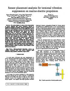
Fig. 1. Hanoi water network. 2. PROBLEM DESCRIPTION A water network can be interpreted as a graph (N , L) where the nodes N = N t ∪N j are either tanks or junctions (the former are flow sources, the latter distribute the existing flow to users and connecting pipes) and edges lij ∈ L which are the pipes linking nodes (e.g., lij denotes a pipe between i, j ∈ N ). For further use we note 1 |N j | = n. 2.1 Network dynamics From our point of view, the characteristic of a junction node i ∈ N j is its pressure pi (t). This characteristic is influenced by the network structure, user demand and, not in the least, by external perturbations (e.g., junction leakages). While in theory the pressure evolution p˙i (t) = gi1 (pi (t)) + gi2 (pj (t)), ∀j s.t. lij ∈ L (1) can be described analytically, the associated nonlinear dynamics are impractical to use (Casillas et al., 2013). An idea is to measure the pressure values against some known nominal value (usually taken in the middle of the night when user demand can be ignored) in order to detect abnormal behavior. Unfortunately, the sensors used for measuring the pressure are expensive to buy and install. Coupled with the fact that real-life networks may have thousands of nodes it becomes clear that only a limited number of junctions can be observed directly. Consequently, the main question becomes how to place this limited number of sensors such that leakage events are correctly identified as much as possible. To answer these questions, hereinafter we make use of the EPANET software (Rossman (2000)), a standard tool for water network emulation. As a particular benchmark (also used routinely in the community) we consider the Hanoi water network (Casillas et al. (2013)). An illustration of this network is given in Fig. 1. The main characteristics are as follows: one tank and 31 junction nodes linked through Hereafter, notation |X| denotes the cardinality of set X, i.e., its number of elements.

1

34 pipes (each of them with a certain length and diameter); each junction node can be affected by a leakage (taking values from within a predefined range) and some of the nodes will have sensors mounted on them (see the figure legend for a representation of each of these elements). 2.2 Fault scenarios The junction node pressure can be affected by a node leakage. We interpret such an event as a fault, that is, a junction node i ∈ N j can be affected by a fault event fi (t) ∈ {0, 2, 3, . . . 33} L/min (2) where ‘0’ stands for healthy functioning and the remaining non-zero values stand for faulty functioning with various fault magnitudes 2 . For further use we partition magnitudes (2) into three disjoint sets: {0}, Itrain = {2, 4, . . . , 32} and Itest = {3, 5, . . . , 33}. We also note m = |Itrain | = |Itest |. A typical fault scenario consists of one (or multiple) faults affecting junction nodes either directly or through propagation. Hence, (1) becomes: p˙i (t) = gi1 (pi (t), fi (t)) + gi2 (pj (t), fj (t)), ∀j s.t. lij ∈ L, (3) where fi (t) affects the current node and the terms pj (fj ) gather the influences of the other nodes (healthy or faulty), as they are transmitted through the network’s pipes. To detect and isolate a fault we require residual signals (Blanke et al. (2006)) which emphasize the faults’ effect and minimize other influences. Hence, for a junction node ni we consider ri (t) = pi (t) − p¯i (4) where p¯i corresponds to a stationary pressure value, measured when the network is under healthy functioning and the external disturbances are reduced to a minimum (no user demand). For further use we define p(t) = ⊤ ⊤ [. . . pi (t) . . .] ∈ Rn , p ¯ = [. . . p¯i . . .] ∈ Rn and r(t) = ⊤ [. . . r(t) . . .] ∈ Rn . 2

We have abused the notation and used fi (t) both as a fault signal and as a magnitude measurement.

255

f5 = 11

6 4

64

f12 = 29

128

0 25 20 15 10 5 0 25 20 15 10 5 0

192

2

dictionary index

f27 = 17

1

fault at n27 fault at n12 fault at n5

8

active atoms 1

2

3

4

5

6

7

8

9 10 11 12 13 14 15 16 17 18 19 20 21 22 23 24 25 26 27 28 29 30 31 f5

f12

f27

Fig. 2. Fault detection and isolation via dictionary classification with sensor placement in the Hanoi water network. 3. MAIN IDEA Since a model-based approach is impractical (due to the network size and its underlying nonlinear dynamics) we consider here a numerical approach. We use Fig. 2 to illustrate the reasoning.

3.1 Dictionary learning elements In our study we use SR for sensor placement. Let y be an observed dense signal and A an overcomplete feature base, that is known and fixed, such that minimize y = Ax x (5) subject to ∥x∥0 ≤ s,

In the three stacked sub-plots of Fig. 2 we have illustrated the residuals (4) for each of the 31 junction nodes for three fault scenarios: leakage in nodes 5, 12 and 27 (not happening simultaneously), each of them for fault magnitudes fi ∈ Itrain . As expected, the residual values are largest in the node directly affected by the fault (red markers) and increase proportionally with the fault magnitude.

where ∥.∥0 is the ℓ0 pseudo-norm counting the non-zero elements of x and s is the sparsity constraint. To solve the sparse representation problem in (5) we need to find the support Is consisting of at most s columns from A and the corresponding coefficients.

Clearly, if each node would have a sensor, the leakage localization would be easily decided. Assuming instead a limited number of sensors (e.g., s = 4), the question becomes which is the best node placement such that as many as possible faults are detected and isolated 3 . The sensor locations illustrated in the figure are {9 ,12, 15 and 30} and are obtained as the result of selecting the most “popular” locations with a classification procedure. These represent the measured subset of residuals and will be the only information further used.

Dictionary learning improves SR by learning the base A from (5) for specific signal classes. Starting from a large set of training data Y ∈ Rp×m , the DL problem tries to find an overcomplete base that is commonly denoted by D ∈ Rp×n , with p < n, called dictionary, that can sparsely represent each data-item by using just a few columns (also called atoms) from the dictionary. Given the sparsity constraint s, we formally express this as the optimization problem minimize ∥Y − DX∥2F D,X

The solution, as detailed in the rest of the paper, is to construct a dictionary of atoms (255 in this example) over which we project the measured residual values with a sparsity constraint. That is, each of the measured residuals is expressed as a combination of a limited number of atoms (i.e., active atoms). These active combinations are in fact a fault signature which uniquely characterizes a certain fault (and its magnitude). This is graphically depicted in the right-most plot of Fig. 2: the blue solid markers denote all atoms which are active for all possible fault magnitudes for a given node. As it can be seen, there are clear differences between the subsets of active atoms. If we assume particular fault magnitudes, e.g, f5 = 11, f12 = 29 and f27 = 17 L/min (black lines in the three stacked left-plots) the uniqueness of the active atoms becomes clear (the hollow black circles in the right-most plot).

subject to

(6)

where ∥.∥F is the Frobenius norm, X ∈ Rn×m are the resulting sparse representations of the signals Y . We normalize all atoms Dj to avoid the multiplication ambiguity resulting from the DX factorization. We can adapt the dictionary D to be better suited for classification by specializing subgroups of atoms to act as labels for a particular class (i.e., for a particular fault, regardless of its magnitude). This is useful when performing fault detection for water network systems, but also for analyzing various sensor placement scenarios. To that end, LC-KSVD (Jiang et al. (2013)) obtains such discriminative dictionaries by regularizing the objective in eq. (6): minimize

∥Y − DX∥2F + α∥Q − AX∥2F +

subject to

+ β∥H − W X∥2F ∥Xi ∥0 ≤ s, i = 1 : m ∥Dj ∥2 = 1, j = 1 : n,

D,X,A,W

3

We are interested in isolating the fault-affected node, not about the magnitude of the fault since, once the leakage is localized, the repair team will in any case assess the magnitude.

∥Xi ∥0 ≤ s, i = 1 : m ∥Dj ∥2 = 1, j = 1 : n,

(7)

3.2 Sensor placement algorithm OMP iteratively solves (5) by selecting at each step the atom that correlates the most with the current residual and then projects the signal to the span of the selected atoms. In the following OMP will be used for sensor placement analysis. In our water network, given a network of n nodes, we want to isolate the fault as best as possible with a few given sensors that we conveniently denote with s. Recalling the definition of (4) and the related terms, taking the m fault magnitudes from Itrain , we organize the residuals as columns inside the residue matrix R ∈ Rn×nm R = [r1,1 r1,2 . . . r1,m | . . . |rn,1 rn,2 . . . rn,m ] . (8) The matrix is divided into n blocks, in which each column represents the residuals for each of the m fault magnitudes (i.e., ri,j is the residual associated with a fault of magnitude ‘j’ affecting the i-th node). Recalling Fig.2, R reflects the network topology with most pressure changes taking place in the affected node and its closest neighbours, while distant nodes have small or insignificant fluctuations. Thus the significant entries, or support, of each column from R are almost the same within one node block and their value varies based on the fault magnitude. The simulated data in R was collected as if we had a pressure sensor in every network node. When dealing with less ideal scenarios s ̸= n, for each column r of R we use OMP to find its vector approximation x by reformulating (5) as minimize ∥r − In x∥22 x (9) subject to ∥x∥0 ≤ s. Using the standard basis as the fixed dictionary comes naturally: when s = n we get pressure data from each node x = r and, when s < n, OMP selects a subset of unit vectors from In that model r best, which is equivalent to performing sensor placement for this specific data-item. The end result is a matrix X ∈ Rn×nm whose columns use at most s atoms from In to approximate the corresponding vectors from R. Graphically, the result of the iterative application of (9) leads to Fig. 3. The i-th row corresponds to the i-th atom (or in other words “sensor placed at the i-th position”) and the number of non-zero entries tells how many times it has been used in the description of the residuals from (8). Conversely, the j-th column puts in evidence the

dictionary atoms

dictionary atoms

31 29 27 25 23 21 19 17 15 13 11 9 7 5 3 11

32

63

94

125 156 187 218 249 280 311 342 373 404 435 466 496 residuals

combination of sensor placements. The decision on how to select overall the “best” s sensors can be taken in multiple ways. In here we considered: (1) Count how many times each atom appears and select the first ‘s’ most common; (2) From each block of m columns (corresponding to the m different magnitudes affecting a given node) take the most ‘s’ frequently used atom; of the ‘n · s’ atoms, select again the first ‘s’. Applying these selection procedures to the example from Fig. 3 leads in case 1 to sensor placement in nodes {15, 12, 30, 9} and in case 2 to {22, 26, 12, 31}. Fig. 4 illustrates the selected nodes (filled circle denotes case (1) and hollow circle denotes case (2)). We observe that repeating for various number of sensors (s = 2 : 10) there is significant variation in the node selection with respect to the number of sensors (and between the two selection procedures considered). 10 9 8 7 6 5 4 3 2

number of sensors

where the first penalty term adds consistent labeling properties to the sparse entries of each sparse code Xi and the second reduces classification error by learning the linear operator W . Each column i of the binary matrix Q has non-zero entries in the places where the input signal Yi and the atom Di share the same label. Thus matrix A is a linear transformation encouraging discrimination in the sparse representations X. For minimizing the classification error, H is built with its columns as standard basis vectors ei where i is the class label of the corresponding training signal from Y . The resulting matrix W represents the classifier parameters.

23 21 19 s = 4 most17 significant atoms which approximate the corresponding residual signal from (8). 15 13 11 9 7 5 3 Fig. 3. Dictionary classification for sensor placement (the case s = 4). 11 32 63 94 125 15 As seen in the figure, each residual “proposes” a different

case (a) case (b)

1 2 3 4 5 6 7 8 9 10 11 12 13 14 15 16 17 18 19 20 21 22 23 24 25 26 27 28 29 30 31

selected nodes

Fig. 4. Node placement selection for different number of sensors. 3.3 Fault detection and isolation implementation The fault detection and isolation step requires again the tools of Section 3.1. This time we obtain simultaneously both the dictionary and the indices of its active atoms for a given measured residual as in (7). For training we use the measured residual matrix (the rows from (8) which correspond to sensor placements, as obtained in Section 3.2). This will lead, as the result of optimization problem (7), to a dictionary which discriminates between 31 classes (one per each fault). For illustration purposes we use parameters α = 4, β = 2, dictionary size n = 248 and number of active atoms is 30

Up to now we have illustrated the fault detection and isolation for a specific number of sensors (s = 4). We are interested to test the performance of the training and subsequent classification for a varying number of sensors and placement strategies. To this end, we consider the data from Fig. 4 and obtain the results shown in Table 1, where the number of sensors varies (s ∈ {2 . . . 10}) and the percentage of successful FDI is shown for each of the two sensor placement strategies described in Section 3.2.

per measured residual. In Fig 5 we show the active (solid circle) atoms for each residual vector. In the detail plot we can see the active atoms for the faults corresponding to node 17. As it can be seen, the active atoms remain largely unchanged (regardless of the fault magnitude) and the resulting support is unique with respect to the other faults (i.e., the combination of atoms {8, 29, 36, 38, 41, 113, 179} uniquely characterizes the fault in node 17). 248

s (1) (2)

187

2 73.0 57.9

3 88.3 86.1

4 85.9 86.3

5 88.7 83.3

6 80.4 86.5

7 85.9 89.5

8 89.3 88.9

9 87.7 90.9

10 80.0 89.5

Table 1. Successful FDI percentage for sensor placement cases 1 and 2.

156 125

We proceed with an overview of the steps required for the initial network setup and for performing online fault detection and isolation.

94

fau

63

lt in

active dictionary atoms

218

The first part is described by Algorithm 1 which handles sensor placement and dictionary learning for fault detection and isolation. Step 1 uses one of the two strategies for sensor placement, described earlier, to obtain the set of nodes Is where the given s sensors will be mounted. We then construct the training data RIs by eliminating the rows from the residual matrix R corresponding to the nodes without sensors. Step 2 is required so that RIs mimics the data we will receive from the sensors when the water system is running. Step 3 trains the dictionary D and the linear classifier W based on the residues RIs , using parameters α and β for tweaking the DL regularization as described around eq. (7).

no

32

de

1

81

161

241

17

1

321

401

481

training residuals

285 281 277 273 1

32

63

94

8 29 36 38 41

125

156

113

187

218

248

179

Fig. 5. Active atoms for residual vectors in the Hanoi network (with detail for the fault 17). With the fault signatures thus obtained it is now possible to test whether different residual signals can be correctly classified (i.e, if the fault affecting them is correctly isolated). To do so, and similarly with (8), we construct residuals (4) but this time for fault magnitudes taken from Itest . We depict in Fig. 6 the projection of the residual corresponding to fault f17 = 17 and observe that the signature of active atoms closely resembles the signature obtained for fault f17 in Fig. 5. That is, the active atoms are {29, 38, 113 and 179} with weights {−0.128, 0.0027, 0.0013, 3.5619} (in the figure we scaled x 7→ log |x| to better highlight the weights of the active atoms) which are 4 of the 7 atoms characterizing the class of fault f17 . Therefore we can conclude that the test residual indeed corresponds to this fault.

Algorithm 1: Placement and FDI learning Data: training residuals R ∈ Rn×nm parameters s, α, β Result: dictionary D, classifier W , sensor nodes Is 1 2 3

Select s sensor nodes Is based on matrix R as in Section 3.2; Let RIs be the restriction of R to the rows in Is ; Use RIs , α and β to learn D and W from (7); Algorithm 2 is used for fault detection and isolation. Given mn residuals obtained with (4) from the s placed sensors, we start by computing the discriminative sparse representations Xk using the learned dictionary D for each residue Rk (step 2). Step 3 applies the linear classifier W and produces the label vector Lk ∈ Rn . The position c of its largest entry corresponds to the predicted class (or node) where the fault took place (Step 3).

2

Algorithm 2: Fault detection and isolation Data: testing residuals R ∈ Rs×mn dictionary D, classifier W Result: prediction P ∈ NK

0 −2 −4 −6

1

−8

2

1

32

63

94

125

156

187

218

248 3 4

Fig. 6. Active atoms for residual vector corresponding to fault f17 = 17.

5

for k = 1 to mn do Use OMP in (5) to obtain Xk using Rk and D ; Label: Lk = W Xk ; Classify: Pk = arg maxc Lk ; end

4. ADDITIONAL RESULTS

ACKNOWLEDGEMENTS

While the previous scheme has given satisfactorily results we are interested in additional use cases. Some of them are discussed below.

This work was supported by the Romanian National Authority for Scientific Research, CNCS - UEFISCDI, project number PN-II-RU-TE-2014-4-2713.

4.1 Network partitioning

REFERENCES

From a practical point of view (i.e., repairing a detected leakage) it makes sense to divide the network into parts combining adjacent nodes. Taking into account the length of the pipes we consider then the partitioning (also depicted in Fig. 1, dashed contours): {1, 2, 3, 4, 16, 17, 18}, {5, 6, 7, 8, 13, 14, 15}, {9, 10, 11, 12}, {19, 20, 21, 22}, {23, 24, 25, 26, 27, 28, 29, 30, 31}. In this case, the fault is associated with the nodes of a partition (hence we have 5 composite faults, one per each partition). Implementation-wise this means that the dictionary from (7) is not trained to discern between the nodes of a partition (since they are of the same class). Note that the dictionary training takes into account the partitioning, it is not simply a grouping of nodes to cover observed wrong FDI labeling (i.e., the dictionary atoms are re-computed and the number of classes is changed from 31 to 5). The result of applying the procedure 4 as in Table 1 leads to the results of Table 2: s (1) (2)

2 96.2 94.0

3 94.2 95.

4 97.0 96.2

5 97.2 96.4

6 97.2 95.6

7 96.6 96.2

8 85.1 96.2

9 96.2 96.0

10 100.0 98.2

Table 2. Successful FDI percentage for sensor placement cases 1 and 2 – with network partitioning. As it can be seen, the success coefficient is significantly larger. The drawback is of course that the fault cannot be localized to a single node. 4.2 Staggered sensor deployment Another aspect of practical interest is the sensor deployment. Assuming that some of the network nodes already have sensors, the question arises of how to place the additional sensors such that overall the FDI accuracy increases. This is tested by considering two scenarios: i) place s = s′ + s′′ in one step and ii) place s′ and after, the remaining s′′ . We take s′ = 4 and s′′ = 3 and observe that in case (i) the selected nodes are {9, 28, 12, 31, 24, 7, 25} with an FDI accuracy of 89.7% whereas in case (ii) we obtain {9, 30, 12, 15} and then {29, 8, 10} with an overall FDI accuracy of 89.3%. We note that the selections differ but still the accuracy FDI is nearly the same. 5. CONCLUSION We have shown that classification and dictionary learning can be adapted to the the twin problems of sensor placement and leakage isolation in a water network. The results have shown good accuracy and pointed towards some promising directions of study like: network partitioning, tweaking of the dictionary learning procedure, and alternative sensor placement strategies. 4

The sensor selections are the same as in the first case since this part of the algorithm does not change.

Aharon, M., Elad, M., and Bruckstein, A. (2006). KSVD: An Algorithm for Designing Overcomplete Dictionaries for Sparse Representation. Signal Processing, IEEE Transactions on, 54(11), 4311–4322. doi: 10.1109/TSP.2006.881199. Araujo, L., Ramos, H., and Coelho, S. (2006). Pressure control for leakage minimisation in water distribution systems management. Water Resources Management, 20(1), 133–149. Blanke, M., Kinnaert, M., Lunze, J., and Staroswiecki, M. (2006). Diagnosis and fault-tolerant control. Springer. Casillas, M.V., Puig, V., Garza-Castan´on, L.E., and Rosich, A. (2013). Optimal sensor placement for leak location in water distribution networks using genetic algorithms. Sensors, 13(11), 14984–15005. Davenport, M.A. and Wakin, M.B. (2010). Analysis of orthogonal matching pursuit using the restricted isometry property. IEEE Transactions on Information Theory, 56(9), 4395–4401. Dziwoki, G. (2016). Averaged properties of the residual error in sparse signal reconstruction. IEEE Signal Processing Letters, 23(9), 1170–1173. Jiang, Z., Lin, Z., and Davis, L.S. (2013). Label consistent K-SVD: Learning a discriminative dictionary for recognition. IEEE Transactions on Pattern Analysis and Machine Intelligence, 35(11), 2651–2664. Ocampo-Martinez, C. and Negenborn, R. (2015). Transport of Water versus Transport over Water. Springer. Pati, Y.C., Rezaiifar, R., and Krishnaprasad, P.S. (1993). Orthogonal matching pursuit: Recursive function approximation with applications to wavelet decomposition. In Conference Record of The 27th Asilomar Conference on Signals, Systems and Computers, 1–3. P´erez, R., Puig, V., Pascual, J., Peralta, A., Landeros, E., and Jordanas, L. (2009). Pressure sensor distribution for leak detection in barcelona water distribution network. Water science and technology: water supply, 9(6), 715– 721. Perez, R., Sanz, G., Puig, V., Quevedo, J., Escofet, M.A.C., Nejjari, F., Meseguer, J., Cembrano, G., Tur, J.M.M., and Sarrate, R. (2014). Leak localization in water networks: A model-based methodology using pressure sensors applied to a real network in Barcelona. IEEE Control Systems, 34(4), 24–36. Rossman, L.A. (2000). EPANET 2: Users Manual. US Environmental Protection Agency. Office of Research and Development. National Risk Management Research Laboratory. Siljak, D.D. (2011). Decentralized control of complex systems. Courier Corporation. Tosic, I. and Frossard, P. (2011). Dictionary Learning. IEEE Signal Proc. Mag., 28(2), 27–38. Ulanicki, B., Kahler, J., and See, H. (2007). Dynamic optimization approach for solving an optimal scheduling problem in water distribution systems. Journal of Water Resources Planning and Management, 133(1), 23–32.