Hindawi Publishing Corporation Mathematical Problems in Engineering Volume 2013, Article ID 419372, 14 pages http://dx.doi.org/10.1155/2013/419372
Research Article Differential Evolution Algorithm with Self-Adaptive Population Resizing Mechanism Xu Wang and Shuguang Zhao College of Information Science and Technology, Donghua University, Shanghai 201620, China Correspondence should be addressed to Xu Wang;
[email protected] Received 4 December 2012; Revised 30 January 2013; Accepted 30 January 2013 Academic Editor: Yang Tang Copyright © 2013 X. Wang and S. Zhao. This is an open access article distributed under the Creative Commons Attribution License, which permits unrestricted use, distribution, and reproduction in any medium, provided the original work is properly cited. A differential evolution (DE) algorithm with self-adaptive population resizing mechanism, SapsDE, is proposed to enhance the performance of DE by dynamically choosing one of two mutation strategies and tuning control parameters in a self-adaptive manner. More specifically, more appropriate mutation strategies along with its parameter settings can be determined adaptively according to the previous status at different stages of the evolution process. To verify the performance of SapsDE, 17 benchmark functions with a wide range of dimensions, and diverse complexities are used. Nonparametric statistical procedures were performed for multiple comparisons between the proposed algorithm and five well-known DE variants from the literature. Simulation results show that SapsDE is effective and efficient. It also exhibits much more superiorresults than the other five algorithms employed in the comparison in most of the cases.
1. Introduction Evolutionary algorithms (EAs), inspired by biological evolutionary mechanism in nature, have achieved great success on many numerical and combinatorial optimizations in diverse fields [1–3]. During the past two decades, EAs have become a hot topic. When implementing the EAs, users need to solve several points, for example, the appropriate encoding schemes, evolutionary operators, and the suitable parameter settings, to ensure the success of the algorithms. The earlier EAs have some disadvantages, such as complex procedure, stagnation, and poor search ability. To overcome such disadvantages, on one hand, some researchers proposed other related methods (e.g., particle swarm optimization (PSO) [4, 5], differential evolution (DE) [6]) which have better global search ability. On the other hand, the effects of setting the parameters of EAs have also been the subject of extensive research [7] by the EA community, and recently there are substantial self-adaptive EAs, which can adjust their parameters along with iterations (see, e.g., [2, 8] for a review). DE is proposed by Storn and Price [6]. Like other EAs, DE is a population-based stochastic search technique as well,
but it is simpler and it can be implemented more easily than other EAs. Besides that, DE [9, 10] is an effective and versatile function optimizer. Owing to simplicity of code, practitioners from other fields can simply apply it to solve their domain-specific problems even if they are not good at programming. Moreover, in traditional DE, there are only three crucial control parameters, that is, scaling factor 𝐹, crossover rate 𝐶𝑟 , and population size NP, which are fewer than other EAs’ (e.g., [8, 11]). It is clear that the appropriate settings of the three control parameters ensure successful functioning of DE [12]. However, results in [6, 13] potentially confuse scientists and engineers who may try to utilize DE to solve scientific and practical problems. Further, while some objective functions are very sensitive to parameter settings, it will be difficult to set the parameter values according to prior experience. Hence, a great deal of publications [14–21] have been devoted to the adjustment of parameters of variation operators. Brest et al. [15] proposed a self-adaptive differential evolution algorithm (called 𝑗DE) based on the self-adapting control parameter scheme, which produced control parameters 𝐹 and 𝐶𝑟 into a new parent vector and adjusted them with probability. Qin et al. in [20, 21] proposed a SaDE algorithm, in which there was
2 a mutation strategy candidate pool. Specifically, in SaDE algorithm, one trial vector generation strategy and associated parameter (𝐹 and 𝐶𝑟 ) settings were adjusted according to their previous experiences of generating promising solutions. Moreover, researchers developed the performance of DE by applying opposition-based learning [22] or local search [23]. In most existing DEs, the population size remains constant over the run. However, there are biological and experimental reasonings to expect that a variable population size would work better. In a natural environment, population sizes of species change and incline to steady state due to natural resources and ecological factors. Technically, the population size in a biological system is the most flexible element. And it can be calibrated more easily than recombination. B¨ack et al. [24] have indicated that calibrating the population size during iterative process could be more rewarding than changing the operator parameters in genetic algorithms. Unfortunately, the DEs with variable population size (e.g., [25, 26]) have not received much attention despite their various applications in real world, and there is still a lot of research space. Hence in this paper, we will focus on DE with variable population size scheme in which the population size can be adjusted dynamically based on the online solution-search status. In this algorithm, we introduce three population adjustment mechanisms to obtain the appropriate value of 𝑁𝑃 according to the desired population distribution. Specifically, while the fitness is improved, it may increase the population size to explore. While short term lacks improvement, it may sink the population size. But if stagnation is over a longer period, the population will grow again. Along with those, two trial vector generation strategies will be adopted adaptively during evolution process. The remainder of this paper is organized as follows. Section 2 gives a brief review of traditional DE and JADE algorithms. Section 3 introduces the DE with self-adaptive population size scheme—SapsDE. Our mutating and adaptive resizing strategies will also be described. Section 4 describes our studies compared with the traditional DE and several state-of-the-art adaptive DE variants and presents the experimental results on a diverse set of test functions with up to 100 dimensions. Finally, Section 5 concludes this paper with some remarks and future research directions.
2. Differential Evolution and JADE Algorithm In this section, we present an overview of the basic concepts of DE and JADE algorithm necessary for a better understanding of our proposed algorithm. 2.1. Differential Evolution. DE is a population-based algorithm, and a reliable and versatile function optimizer, which evolves a population of NP D-dimensional individuals towards the global optimum by enhancing the differences of the individuals. In brief, after initialization, DE repeats mutation, crossover, and selection operations to produce a trail vector and select one of those vectors with the best fitness value for each vector until satisfying some specific
Mathematical Problems in Engineering termination criteria. Conveniently, subsequent generation in DE is denoted by 𝐺 = 0, 1, . . . , 𝐺max . We notate the 𝑖th vector of the population at the current generation as follows: 𝐺 𝐺 𝐺 𝐺 , 𝑥𝑖,2 , . . . , 𝑥𝑖,𝑗 ), 𝑋⃗ 𝑖 = (𝑥𝑖,1
𝑗 = 1, 2, . . . , 𝐷.
(1)
Initialization. First of all, uniformly randomize NP individuals within a D-dimensional real parameter search space. And the initial population should cover the entire search space constrained by the prescribed minimum and maximum bounds: 𝑋⃗ min = (𝑥min,1 , 𝑥min,2 , . . . , 𝑥min,𝐷), 𝑋⃗ max = (𝑥max,1 , 𝑥max,2 , . . . , 𝑥max,𝑗 ). Hence, the initialization of the 𝑗th element in the 𝑖th vector is taken as follows: 0 = 𝑥min,𝑗 + rand (0, 1) ⋅ (𝑥max,𝑗 − 𝑥min,𝑗 ) , 𝑥𝑖,𝑗
𝑗 = 1, 2, . . . , 𝐷,
(2)
where rand(0, 1) represents a uniformly distributed random variable within the range [0, 1], and it is instantiated independently for each component of the 𝑖th vector. Mutation Operation. In the existing literature on DE, mutate vector 𝑉𝑖 , called donor vector, is obtained through the differential mutation operation with respect to each individual 𝑋⃗ 𝑖 , known as target vector, in the current population. For each target vector from the current population, the donor vector is created via certain mutation strategy. Several mutation strategies have been proposed. Here we list one of the most popular and simplest forms of DE-mutation as follows: 𝐺 𝐺 𝐺 𝐺 𝑉⃗ 𝑖 = 𝑋⃗ 𝑟1 + 𝐹 ⋅ (𝑋⃗ 𝑟2 − 𝑋⃗ 𝑟3 ) .
(3)
The indices 𝑟1 , 𝑟2 , and 𝑟3 are mutually exclusive integers randomly generated within the range [1, 𝑁𝑃], which are different from the base vector index 𝑖. These indices are randomly generated for each mutant vector. Now, the difference of any two of these three vectors is scaled by a mutation weighting factor 𝐹 which typically lies in the interval [0.4, 1] in the existing DE literature, and the scaled difference is added to the third one to obtain a donor vector V. Crossover Operation. After the mutation operation, according 𝐺 to the target vector 𝑋⃗ and its corresponding donor vector 𝑖
𝐺 𝐺 𝑉⃗ 𝑖 , a trail vector 𝑈⃗ 𝑖 is produced by crossover operation. In traditional version, DE applies the binary defined crossover as follows:
𝐺 𝑢𝑖,𝑗
𝐺 {V𝑖,𝑗 , if rand𝑖,𝑗 [0, 1] ≤ 𝐶𝑟 or 𝑗 = 𝑗rand , ={ 𝐺 𝑥 , otherwise, { 𝑖,𝑗
(4)
where 𝐶𝑟 is a crossover rate within the range [0, 1], defined by user as a constant, which controls the probability of
Mathematical Problems in Engineering
3
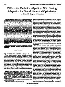
(1): Begin (2): Initialization(); Generate uniformly distributed random population of NP individuals (3): while stopping criterion is not satisfied do (4): for 𝑖 = 1 to NP do (5): Select random indexes 𝑟1 , 𝑟2 , 𝑟3 𝑤𝑖𝑡ℎ 𝑟1 ≠ 𝑟2 ≠ 𝑟3 ≠ 𝑖 𝐺 𝐺 𝐺 𝐺 (6): 𝑉⃗ 𝑖 = 𝑋⃗ 𝑟1 + 𝐹 ⋅ (𝑋⃗ 𝑟2 − 𝑋⃗ 𝑟3 ) (7): 𝑗rand = [rand [0, 1) ∗ 𝐷] (8): for𝑗 = 1 to 𝐷 do (9): if rand𝑖,𝑗 [0, 1] ≤ 𝐶𝑟 𝑜𝑟 𝑗 = 𝑗rand then 𝐺 𝐺 = V𝑖,𝑗 (10): 𝑢𝑖,𝑗 (11): else 𝐺 𝐺 (12): 𝑢𝑖,𝑗 = 𝑥𝑖,𝑗 (13): end if (14): end for 𝐺 𝐺 (15): if𝑓(𝑈⃗ 𝑖 ) ≤ 𝑓(𝑋⃗ 𝑖 ) then 𝐺+1 𝐺 (16): 𝑋⃗ 𝑖 = 𝑈⃗ 𝑖 (17): else 𝐺+1 𝐺 (18): 𝑋⃗ 𝑖 = 𝑋⃗ 𝑖 (19): end if (20): end for (21): G=G+1 (22): end while (23): End
Algorithm 1: Differential evolution algorithm.
parameter values employed from the donor vector. 𝑗rand is a randomly chosen integer within the range [1, 𝑁𝑃] which is introduced to ensure that the trial vector contains at least one parameter from donor vector. Selection Operation. In classic DE algorithm, a greedy selection is adopted. The fitness of every trail vectors is evaluated and compared with that of its corresponding target vector in the current population. For minimization problem, if the fitness value of trial vector is not more than that of target vector, the target vector will be replaced by the trial vector in the population of the next generation. Otherwise, the target vector will be maintained in the population of the next generation. The selection operation is expressed as follows: 𝐺+1 𝑋⃗ 𝑖
𝐺 𝐺 𝐺 {𝑈⃗ , if 𝑓 (𝑈⃗ 𝑖 ) ≤ 𝑓 (𝑋⃗ 𝑖 ) , = { 𝑖𝐺 ⃗ {𝑋𝑖 , otherwise.
(5)
𝐹𝑖 = rand 𝑐𝑖 (𝜇𝐹 , 0.1) , 𝐶𝑟𝑖 = rand 𝑛𝑖 (𝜇𝐶𝑟 , 0.1) .
(7)
The proposed two location parameters are initialized as 0.5 and then generated at the end of each generation as follows:
The algorithmic process of DE is depicted in Algorithm 1.
𝜇𝐹 = (1 − 𝑐) ⋅ 𝜇𝐹 + 𝑐 ⋅ mean𝐿 (𝑆𝐹 ) ,
2.2. JADE Algorithm. Zhang and Sanderson [27] introduced adaptive differential evolution with optional external archive, named JADE, in which a neighborhood-based mutation strategy and an optional external archive were employed to improve the performance of DE. It is possible to balance the exploitation and exploration by using multiple best solutions, called DE/current-to-pbest strategy, which is presented as follows: 𝐺 𝐺 𝐺 𝐺 ̃𝐺 v𝐺 𝑖 = x𝑖 + 𝐹𝑖 ⋅ (xbest,𝑝 − x𝑖 ) + 𝐹𝑖 ⋅ (x𝑟1 − x 𝑟2 ) ,
𝐺 is randomly selected as one of the top 100 where xbest,𝑝 p% individuals of the current population with 𝑝 ∈ (0, 1]. Meanwhile, x𝑖𝐺 and x𝑟𝐺1 are diverse and random individuals in the current population P, respectively. x̃𝐺 𝑟2 is randomly selected from the union of P and the archive A. In Particular, A is a set of achieved inferior solutions in recent generations and its individual number is not more than the population size. At each generation, the mutation factor 𝐹𝑖 and the crossover factor 𝐶𝑟𝑖 of each individual x𝑖 are, respectively, updated dynamically according to a Cauchy distribution of mean 𝜇𝐹 and a normal distribution of mean 𝜇𝐶𝑟 as follows:
(6)
𝜇𝐶𝑟 = (1 − 𝑐) ⋅ 𝜇𝐶𝑟 + 𝑐 ⋅ mean𝐴 (𝑆𝐶𝑟 ) ,
(8)
where 𝑐 in (0, 1) is a positive constant; 𝑆𝐹 /𝑆𝐶𝑟 indicates the set of all successful mutation/crossover factors in generation; mean𝐴(⋅) denotes the usual arithmetic mean, and mean𝐿 (⋅) is the Lehmer mean, which is defined as follows: |𝑆 |
mean𝐿 (𝑆𝐹 ) =
∑𝑖=1𝐹 𝐹𝑖2 |𝑆 |
∑𝑖=1𝐹 𝐹𝑖
.
(9)
4
Mathematical Problems in Engineering
3. SapsDE Algorithm Here we develop a new SapsDE algorithm by introducing a self-adaptive population resizing scheme into JADE. Technically, this scheme can gradually self-adapt 𝑁𝑃 according to the previous experiences of generating promising solutions. In addition, we use two DE mutation strategies in SapsDE. In each iteration, only one DE strategy is activated. The structure of the SapsDE is shown in Algorithm 2. 3.1. Generation Strategies Chooser. DE performs better if it adopts different trail vector generation strategies during different stages of optimization [21]. Hence, in SapsDE, we utilize two mutation strategies, that is, DE/rand-to-best/1 and DE/current-to-𝑝best/1. The DE/rand-to-best/1 strategy benefits from its fast convergence speed but may result in premature convergence due to the resultant reduced population diversity. On the other hand, the DE/current-to-𝑝best/1 strategy balances the greediness of the mutation and the diversity of the population. Considering the above two strategies, we introduce a parameter 𝜃 to choose one of the strategies in each iteration of the evolutionary process. At an earlier stage of evolutionary process, DE/current-to-best/1 strategy is adopted more to achieve fast convergence speed. For avoiding trapping into a local optimum, as the generation is proceeding further, DE/current-to-𝑝best/1 strategy is used more to search for a relatively large region which is biased toward promising progress directions. As presented in lines 8–15 in Algorithm 2, the DE/randto-best/1 strategy is used when 𝑅𝑛 is smaller than 𝜃; otherwise, DE/current-to-𝑝best/1 strategy is picked where 𝑅𝑛 is a random number generated from the continuous uniform distribution on the interval (0, 1). Notice that 𝜃 ∈ [0.1, 1] is a time-varying variable which diminishes along with the increase of generation and it can be expressed as follows: 𝜃=
(𝐺max − 𝐺) ∗ 𝜃max + 𝜃min , 𝐺max
(10)
where 𝜃min = 0.1, 𝜃max = 0.9, and 𝐺 denotes the generation counter. Hence, DE/rand-to-best/1 strategy can be frequently activated at earlier stage as the random number can easily get smaller than 𝜃. Meanwhile, DE/current-to-𝑝best/1 strategy takes over more easily as the generation increases. 3.2. Population Resizing Mechanism. The population resizing mechanism aims at dynamically increasing or decreasing the population size according to the instantaneous solutionsearching status. In SapsDE, the dynamic population size adjustment mechanism depends on a population resizing trigger. This trigger will activate population-reducing or augmenting strategy in accordance with the improvements of the best fitness in the population. One step further, if a better solution can be found in one iteration process, the algorithm becomes more biased towards exploration augmenting the population size, short-term lack of improvement shrinks the population for exploitation, but stagnation over a longer period causes population to grow again. Further,
the population size is monitored to avoid breaking lower bound. As described in lines 23–34 in Algorithm 2, Lb is the lower bound indicator. Correspondingly, Lbound is the lower bounds of the population size. The proposed 𝐵, 𝑊, and 𝑆𝑡 are three significant trigger variables, which are used to activate one of all dynamic population size adjustment strategies. More specifically, the trigger variable 𝑊 is set to 1 when the best fitness does not improve, that may lead to a populationreducing strategy to delete poor individuals from current population. Furthermore, similarly, if there is improvement of the best fitness, 𝐵 and 𝑆𝑡 are assigned 1, respectively. The population-augmenting strategy 1 is used when the trigger variable 𝐵 is set to 1. Besides, if the population size is not bigger than the lower bound (Lbound) in consecutive generations, the lower bound monitor (𝐿𝑏) variable will be increased in each generation. This process is continuously repeated until it achieves a user-defined value 𝑅; that is, the population-augmenting strategy2 will be applied if 𝐿𝑏 > 𝑅 or 𝑆𝑡 > 𝑅. Technically, this paper applies three population resizing strategies as follows. Population Reducing Strategy. The purpose of the population-reducing strategy is to make the search concentrating more on exploitation by removing the redundant inferior individuals when there is no improvement of the best fitness in short term. More specifically, in population reducing strategy, the first step is to evaluate fitness function values of individuals. Second step is to arrange the population with its fitness function values from small to large. For minimization problems, the smaller the value of fitness function is, the better the individual performs. Consequently, the third step is to remove some individuals with large values from the current population. The scheme of population reduction is presented in Algorithm 3, where 𝜌1 denotes the number of deleted individuals. Population Augmenting Strategy1. Population Augmenting strategy1 is intended to bias more towards exploration in addition to exploitation. Here it applies DE/best/2 mutation strategy to generate a new individual increasing the population size on fitness improvement. The pseudocode of the population-increasing scheme is shown in Algorithm 4. Population Augmenting Strategy2. The population size is increased by population augmenting strategy2, shown in Algorithm 5 if there is no improvement during the last 𝑅 number of evaluations. The second growing strategy is supposed to initiate renewed exploration when the population is stuck in local optima. So, here it applies DE/rand/1 mutation scheme. In theory, the size to increase the population in this step can be defined independently from others, but in fact we use the same growth rate 𝑠 as one of the population-reducing strategy.
4. Experiments and Results 4.1. Test Functions. The SapsDE algorithm was tested on benchmark suite consisting of 17 unconstrained singleobjective benchmark functions which were all minimization problems. The first 8 benchmark functions are chosen from
Mathematical Problems in Engineering
5
(1): Begin (2): 𝐺 = 0 (3): Randomly initialize a population of 𝑁𝑃 vectors uniformly distributed in the (4): range [𝑋min , 𝑋max ] (5): Evaluate the fitness values of the population (6): while termination criterion is not satisfied do (7): for 𝑖 = 1 to 𝑁𝑃 do 𝐺 (8): Generate donor vector 𝑋⃗ 𝑖 (9): if 𝑅𝑛 < 𝜃 then 𝐺 − x𝑖𝐺) + 𝐹𝑖 ⋅ (x𝑟𝐺1 − x̃𝐺𝑟2 ) (10): v𝐺𝑖 = x𝑖𝐺 + 𝐹𝑖 ⋅ (xbest (11): // mutate with DE/rand-to-best/1 strategy (12): else 𝐺 − x𝑖𝐺) + 𝐹𝑖 ⋅ (x𝑟𝐺1 − x̃𝐺𝑟2 ) (13): v𝐺𝑖 = x𝑖𝐺 + 𝐹𝑖 ⋅ (xbest,𝑝 (14): // mutate with DE/current-to-𝑝best/1 strategy (JADE) (15): end if (16): Through crossover operation to generate trial vector 𝐺 (17): 𝑈⃗ 𝑖 = Strategy (𝑖, pop) 𝐺 (18): Evaluate the trial vector 𝑈⃗ 𝑖 𝐺 𝐺 (19): if𝑓(𝑈⃗ 𝑖 ) ≤ 𝑓(𝑋⃗ 𝑖 ) then
𝐺+1 𝐺 (20): 𝑋⃗ 𝑖 = 𝑈⃗ 𝑖 // Save index for replacement (21): end if (22): end for (23): //𝜙 is the minimum value of function evaluations in the last generation (24): //𝐿𝑏 is the low bound of population size 𝐺 (25): if min(𝑓(𝑋⃗ 𝑖 )) < 𝜙 then (26): 𝐵 = 1; 𝐺 (27): 𝜙 = min(𝑓(𝑋⃗ 𝑖 )) (28): else (29): 𝑊 = 1; (30): 𝑆𝑡 = 𝑆𝑡 + 1; (31): end if (32): if popsize ≤ Lbound then (33): 𝐿𝑏 = 𝐿𝑏 + 1 (34): end if (35): if (𝑊 == 1) and (𝑆𝑡 ≤ 𝑅) then (36): Population Reducing Strategy() (37): 𝑊=0 (38): end if (39): if (𝐵 == 1) then (40): Population Augmenting Strategy1() (41): Evaluate the new additional individuals (42): 𝐵=0 (43): 𝑆𝑡 = 0 (44): end if (45): if (𝑆𝑡 > 𝑅) or (𝐿𝑏 > 𝑅) then (46): Population Augmenting Strategy2() (47): Evaluate the new additional individuals (48): 𝑆𝑡 = 0 (49): 𝐿𝑏 = 0 (50): end if (51): 𝐺=𝐺+1 (52): end while (53): End
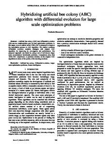
Algorithm 2: The SapsDE algorithm.
6
Mathematical Problems in Engineering
(1): Begin (2): Arrange the population with its fitness function values in ascending order ⃗ 𝑥⃗ 1 ), 𝑓(𝑥⃗ 2 ), . . . , 𝑓(𝑥⃗ 𝑆𝑃 )) = (𝑓min , 𝑓min +1 , . . . , 𝑓max ) (3): F(𝑓( (4): 𝜌1 = ⌊𝑠% × 𝑁𝑃⌋ (5): Remove the last 𝜌1 individuals from current population (6): End Algorithm 3: Population reducing strategy.
(1): Begin (2): Select the best individual from the current population (3): Randomly select four different vectors 𝑥𝑟𝐺1 ≠ 𝑥𝑟𝐺2 ≠ 𝑥𝑟𝐺3 ≠ 𝑥𝑟𝐺4 from the (4): current population 𝐺 𝐺 = 𝑥best + 𝐹 ⋅ (𝑥𝑟𝐺1 − 𝑥𝑟𝐺2 ) + 𝐹 ⋅ (𝑥𝑟𝐺3 − 𝑥𝑟𝐺4 ) (5): 𝑥𝑖,𝑏 𝐺 (6): Store 𝑥𝑖,𝑏 into BA (7): Add the individual of BA into the current population (8): Empty BA (9): End
Algorithm 4: Population augmenting strategy1.
the literature and the rest are selected from CEC 2005 Special Session on real-parameter optimization [28]. The detailed description of the function can be found in [29, 30]. In Table 1, our test suite is presented, among which functions 𝑓1 , 𝑓2 , and 𝑓9 –𝑓12 are unimodal and functions 𝑓3 –𝑓8 and 𝑓13 –𝑓17 are multimodal. 4.2. Parameter Settings. SapsDE is compared with three state-of-the-art DE variants (JADE, 𝑗DE, and SaDE) and the classic DE with DE/rand/1/bin/strategy. To evaluate the performance of algorithms, experiments were conducted on the test suite. We adopt the solution error measure (𝑓(𝑥) − 𝑓(𝑥∗ )), where 𝑥 is the best solution obtained by algorithms in one run and 𝑥∗ is well-known global optimum of each benchmark function. The dimensions (𝐷) of function are 30, 50, and 100, respectively. The maximum number of function evaluations (FEs), the terminal criteria, is set to 10 000 × 𝐷, all experiments for each function and each algorithm run 30 times independently. In our experimentation, we follow the same parameter settings in the original paper of JADE, 𝑗DE, and SADE. For DE/rand/1/bin, the parameters are also studied in [31]. The details are shown as follows: (1) the original DE algorithm with DE/rand/1/𝑏𝑖𝑛 strategy, F = 0.9, 𝐶𝑟 = 0.9 and P (population size) = 𝑁 (dimension); (2) JADE, 𝑝 = 0.05, 𝑐 = 0.1; (3) 𝑗DE, 𝜏1 = 𝜏2 = 0.1; (4) SaDE, 𝐹: rand𝑁(0.5, 0.3), 𝐿𝑃 = 50. For SapsDE algorithm, the configuration is listed as follows: the 𝐿𝑏𝑜𝑢𝑛𝑑 is set to 50. Initial population size is set
to 50. The adjustment factor of population size 𝑠 is fixed to 1. The threshold variable of boundary and stagnation variable 𝑅 is set to 4. All experiments were performed on a computer with Core 2 2.26-GHz CPU, 2-GB memory, and Windows XP operating system. 4.3. Comparison with Different DEs. Intending to show how well the SapsDE performs, we compared it with the conventional DE and three adaptive DE variants. We first evaluate the performance of different DEs to optimize the 30-dimensional numerical functions 𝑓1 (𝑥)–𝑓17 (𝑥). Table 2 reports the mean and standard deviation of function values over 30 independent runs with 300 000 FES. The best results are typed in bold. For a thorough comparison, the two-tailed t-test with a significance level of 0.05 has been carried out between the SapsDE and other DE variants in this paper. Rows “+ (Better),” “= (Same),” and “− (Worse)” give the number of functions that the SapsDE performs significantly better than, almost the same as, and significantly worse than the compared algorithm on fitness values in 30 runs, respectively. Row total score records the number of +’s and the number of –’s to show an overall comparison between the two algorithms. Table 2 presents the total score on every function. In order to further evaluate the performance of SapsDE, we report the results of SapsDE and other four DE variants on test functions at 𝐷 = 50. The experimental results are summarized in Table 3. From Table 2, SapsDE is significantly better than other comparisonal algorithms on thirteen functions while it is outperformed by JADE on functions 𝑓10 and 𝑓12 and by SaDE on functions 𝑓1 and 𝑓17 . Obviously, SapsDE obtains the best average ranking among the five algorithms.
Mathematical Problems in Engineering
7
(1): Begin (2): 𝜌2 = ⌈𝑠% × 𝑁𝑃⌉ (3): Select 𝜌2 best individuals from the current population (4): for 𝑖 = 1 to 𝜌2 do (5): Randomly generate three different vectors 𝑥𝑟𝐺1 ≠ 𝑥𝑟𝐺2 ≠ 𝑥𝑟𝐺3 from the (6): current population 𝐺 (7): 𝑥𝑖,𝑏 = 𝑥𝑟𝐺1 + 𝐹 ⋅ (𝑥𝑟𝐺2 − 𝑥𝑟𝐺3 ) 𝐺 (8): Store 𝑥𝑖,𝑏 into BA (9): end for (10): Add the total individuals of BA into the current population, and empty BA (11): End
Algorithm 5: Population augmenting strategy2.
Table 1: Benchmark functions. Functions 𝑓1 (𝑥) 𝑓2 (𝑥) 𝑓3 (𝑥)
Name
Search space
Sphere Rosenbrock
[−100, 100]
𝐷
[−100, 100]
𝐷
[−32, 32]
Ackley
𝐷
𝑓4 (𝑥)
Griewank
[−600, 600]
𝑓5 (𝑥)
Rastrigin
[−5, 5]𝐷
𝑓6 (𝑥) 𝑓7 (𝑥) 𝑓8 (𝑥) 𝑓9 (𝑥) 𝑓10 (𝑥) 𝑓11 (𝑥)
Generalized Penalized Function 1 Generalized Penalized Function 2 Shifted Sphere Shifted Schwefel’s Problem 1.2 Shifted Rotated High Conditioned Elliptic
𝐷
[−50, 50]
𝐷
[−50, 50]
𝐷
𝑓17 (𝑥)
Shifted Rotated Weierstrass
More specifically, with respect to JADE, the t-test is 4/1/12 in Table 2. It means that SapsDE significantly outperforms JADE on 4 out of 17 benchmark functions. JADE is significantly better than SapsDE on one function 𝑓12 . For the rest of benchmark functions, there is no significant difference between SapsDE and JADE. Similarly, we can get that SapsDE performs significantly better than DE, 𝑗DE, and SaDE on 14, 11, and 14 out of 17 test functions, respectively. Thus, SapsDE is the winner of test. The reason is that SapsDE implements the adaptive population resizing scheme, which can help the algorithm to search the optimum as well as maintaining a higher convergence speed when dealing with complex functions.
0 −450
[−100, 100]
𝐷
−450
𝐷
−450
[−100, 100]𝐷
Shifted Rotated Rastrigin
0
[−100, 100] [−100, 100]
𝑓16 (𝑥)
0
−450
Shifted Rosenbrock Shifted Rastrigin
0
𝐷
Shifted Schwefel’s Problem 1.2 with Noise in Fitness
𝑓15 (𝑥)
0
[−100, 100]
𝑓13 (𝑥)
Shifted Rotated Ackley’s Function with Global Optimum on Bounds
0
𝐷
𝑓12 (𝑥) 𝑓14 (𝑥)
0
0
[−100, 100]
Salomon
𝐷
𝑓bias
[−32, 32]
𝐷
[−100, 100] [−5, 5]
𝐷
𝐷
[−0.5, 0.5]
390 −140 −330 −330
𝐷
90
From Table 3, it can be seen that SapsDE is significantly better than other algorithms on the 14 (𝑓1 –𝑓3 , 𝑓5 , and 𝑓7 –𝑓16 ) out of 17 functions. On the two functions 𝑓4 and 𝑓6 , 𝑗DE outperforms SapsDE. And for test function 𝑓17 , the best solution is achieved by SaDE. Particularly, SapsDE provides the best performance among the five algorithms on all unimodal functions. The three inferior solutions of SapsDE are all on the multimodal functions. However, in general, it offers more improved performance than all of the compared DEs. The t-test is summarized in the last three rows of Table 3. In fact, SapsDE performs better than DE, JADE, 𝑗DE, and SaDE on 16, 8, 11, and 16 out of 17 test functions, respectively. In general, our
8
Mathematical Problems in Engineering Table 2: Experimental results of 30-dimensional problems 𝑓1 (𝑥)–𝑓17 (𝑥), averaged over 30 independent runs with 300 000 FES.
Function
DE
JADE
𝑗DE
SaDE
SapsDE
Mean error (Std Dev)
Mean error (Std Dev)
Mean error (Std Dev)
Mean error (Std Dev)
Mean error (Std Dev)
1.07e − 130 (4.99e − 130)−
4.38𝑒−126 (2.27𝑒−125)
1
8.70𝑒−032 (1.07𝑒−31)+ 8.52𝑒−123 (4.49𝑒−122)+ 2.14𝑒 − 61 (3.68𝑒 − 61)+
2
8.14𝑒 + 07 (5.94𝑒 + 07)+ 9.42𝑒 − 01 (4.47𝑒 − 01)+ 1.18𝑒 + 01 (1.06𝑒 + 01)+ 3.62𝑒 + 01 (3.20𝑒 + 01)+ 1.32e − 01 (7.27e − 01)
3
4.32𝑒 − 15 (1.80𝑒 − 15)+
2.66e − 15 (0.00e + 00)
2.90𝑒 − 15 (9.01𝑒 − 16)= 1.51𝑒 − 01 (4.00𝑒 − 01)+ 2.66e − 15 (0.00e + 00)
4
5.75𝑒−004 (2.21𝑒−03)+
0.00e + 00 (0.00e + 00)
0.00e + 00 (0.00e + 00) 6.14𝑒 − 03 (1.22𝑒 − 02)+ 0.00e + 00 (0.00e + 00)
5
1.33𝑒 + 02 (2.13𝑒 + 01)+
0.00e + 00 (0.00e + 00)
0.00e + 00 (0.00e + 00) 6.63𝑒 − 02 (2.52𝑒 − 01)+ 0.00e + 00 (0.00e + 00)
6
1.89𝑒 − 01 (3.00𝑒 − 02)= 1.90𝑒 − 01 (3.05𝑒 − 02)= 1.97𝑒 − 01 (1.83𝑒 − 02)+ 2.53𝑒 − 01 (7.30𝑒 − 02)+ 1.77e − 01 (3.94e − 02)
7
2.08𝑒 − 32 (1.21𝑒 − 32)+
1.57e − 32 (5.56e − 48)
1.57e − 32 (5.57e − 48) 6.91𝑒 − 03 (2.63𝑒 − 02)+ 1.57e − 32 (5.56e − 48)
8
8.16𝑒 − 32 (8.89𝑒 − 32)+
1.34e − 32 (5.56e − 48)
1.35𝑒 − 32 (5.57𝑒 − 48)+ 1.10𝑒 − 03 (3.35𝑒 − 03)+ 1.34e − 32 (5.56e − 48)
9
0.00e + 00 (0.00e + 00)
0.00e + 00 (0.00e + 00)
0.00e + 00 (0.00e + 00)
0.00e + 00 (0.00e + 00)
0.00e + 00 (0.00e + 00)
10
3.99𝑒 − 05 (2.98𝑒 − 05)+ 1.10e − 28 (9.20e − 29)= 9.55𝑒 − 07 (1.32𝑒 − 06)+ 1.06𝑒 − 05 (3.92𝑒 − 05)+
1.17𝑒 − 28 (1.07𝑒 − 28)
11
1.01𝑒 + 08 (2.13𝑒 + 07)+ 1.06𝑒 + 04 (8.07𝑒 + 03)+ 2.29𝑒 + 05 (1.47𝑒 + 05)+ 5.25𝑒 + 05 (2.099𝑒 + 05)+ 7.00e + 03 (4.29e + 03)
12
1.44𝑒 − 02 (1.33𝑒 − 02)+ 2.33e − 16 (6.61e − 16)− 5.55𝑒 − 02 (1.54𝑒 − 01)+ 2.5.𝑒 + 02 (2.79𝑒 + 02)+
13
2.46𝑒 + 00 (1.61𝑒 + 00)= 3.02𝑒 + 00 (9.38𝑒 + 00)= 1.83𝑒 + 01 (2.04𝑒 + 01)+ 5.74𝑒 + 01 (2.95𝑒 + 01)+ 1.49e + 00 (5.68e + 00)
14
2.09𝑒 + 01 (4.56𝑒 − 02)+ 2.08𝑒 + 01 (2.47𝑒 − 01)= 2.10𝑒 + 01 (4.17𝑒 − 02)+ 2.10𝑒 + 01 (3.46𝑒 − 02)+ 2.07e + 01 (3.98e − 01)
15
1.20𝑒 + 02 (2.64𝑒 + 01)+
16
1.79𝐸 + 02 (9.37𝑒 + 00)+ 2.32𝑒 + 01 (4.08𝑒 + 00)= 5.66𝑒 + 01 (1.00𝑒 + 01)+ 4.62𝑒 + 01 (1.02𝑒 + 01)+ 2.18e + 01 (3.58e + 00)
17
3.92𝑒 + 01 (1.20𝑒 + 00)+ 2.49𝑒 + 01 (2.28𝑒 + 00)+ 2.78𝑒 + 01 (1.87𝑒 + 00)+ 1.72e + 01 (2.53e + 00)− 2.42𝑒 + 01 (1.68𝑒 + 00)
0.00e + 00 (0.00e + 00)
4.22𝑒 − 15 (1.25𝑒 − 14)
0.00e + 00 (0.00e + 00) 1.33𝑒 − 01 (3.44𝑒 − 01)+ 0.00e + 00 (0.00e + 00)
Total score
DE
JADE
𝑗DE
SaDE
SapsDE
+
14
4
11
14
∗
−
0
1
0
2
∗
=
3
12
6
1
∗
proposed SapsDE performs better than other DE variants on benchmark functions at 𝐷 = 50 in terms of the quality of the final results. We can see that the proposed SapsDE is effective and efficient on optimization of low dimensional functions. However, high dimensional problems are typically harder to solve and a common practice is to employ a larger population size. In order to test the ability of the SapsDE in high dimensional problems, we compared it with other four DE variants for our test functions at 𝐷 = 100. In Table 4, the experimental results of 100-dimensional problems 𝑓1 –𝑓17 are summarized. Table 4 shows that the SapsDE provides the best performance on the 𝑓1 , 𝑓2 , 𝑓5 , 𝑓6 , 𝑓8 , 𝑓11 , and 𝑓14 –𝑓17 and performs slightly worse than one of four comparisonal algorithms on the rest of the functions. The 𝑗DE offers the best performance on the 𝑓3 , 𝑓4 , and 𝑓7 . SaDE performs best on the 𝑓9 . However,
the differences between SapsDE and 𝑗DE are considered to be not quite statisfically significant on the 𝑓3 , 𝑓4 , and 𝑓7 , neither does it between SapsDE and SaDE on the 𝑓9 . To apply the t-test, we obtain the statistic results of the experiments at 𝐷 = 100 for all functions. The results of SapsDE are compared with those of DE, JADE, SaDE, and 𝑗DE. Results of t-test are presented in the last three rows of Table 4. It is clear that SapsDE obtains higher “+” values than “−” values in all cases. Unquestionably, SapsDE performs best on 100-dimension benchmark functions. Comparing the overall performances of five algorithms on all functions, we find that SapsDE obtains the best average ranking, which outperforms the other four algorithms. JADE follows SapsDE in the second best average ranking. The 𝑗DE can converge to the best solution found so far very quickly though it is easy to stuck in the local optima. The SaDE has
Mathematical Problems in Engineering
9
Table 3: Experimental results of 50-dimensional problems 𝑓1 (𝑥)–𝑓17 (𝑥), averaged over 30 independent runs with 500 000 FES. Function
DE
JADE
𝑗DE
SADE
SapsDE
Mean error (Std Dev)
Mean error (Std Dev)
Mean error (Std Dev)
Mean error (Std Dev)
Mean error (Std Dev)
1
3.51𝑒 − 35 (4.71𝑒 − 35)+ 1.99𝑒 − 184 (0.00𝑒 + 00)+ 5.98𝑒 − 62 (7.49𝑒 − 62)+ 1.67𝑒−118 (7.81𝑒−118)+ 3.05e − 202 (0.00e + 00)
2
1.82𝑒 + 08 (1.16𝑒 + 08)+ 5.32𝑒 − 01 (1.38𝑒 + 00)+ 2.61𝑒 + 01 (1.56𝑒 + 01)+ 6.79𝑒 + 01 (3.58𝑒 + 01)+ 1.70e − 28 (5.55e − 28)
3
2.69𝑒 − 02 (7.63𝑒 − 03)+ 5.98𝑒 − 15 (9.01𝑒 − 16)= 6.21𝑒 − 15 (0.00𝑒 + 00)+ 1.18𝑒 + 00 (4.68𝑒 − 01)+ 5.38e − 15 (1.52e − 15)
4
6.35𝑒 − 02 (1.62𝑒 − 01)+ 1.56𝑒 − 03 (5.46𝑒 − 03)= 0.00e + 00 (0.00e + 00)− 1.39𝑒 − 02 (3.26𝑒 − 02)+
5
2.02𝑒 + 02 (5.08𝑒 + 01)+
6
1.78𝑒 + 00 (2.00𝑒 − 01)+ 3.07𝑒 − 01 (3.65𝑒 − 02)+ 2.00e − 01 (3.55e − 11)− 5.37𝑒 − 01 (1.13𝑒 − 01)+
7
1.24𝑒 − 02 (4.73𝑒 − 02)+ 6.22𝑒 − 03 (1.90𝑒 − 02)+ 1.57𝑒 − 32 (5.57𝑒 − 48)+ 5.39𝑒 − 02 (1.04𝑒 − 01)+ 9.42e − 33 (2.78e − 48)
8
1.37𝑒 − 32 (9.00𝑒 − 34)= 1.35𝑒 − 32 (5.57𝑒 − 48)= 1.35𝑒 − 32 (5.57𝑒 − 48)= 5.43𝑒 − 02 (2.91𝑒 − 01)+ 1.34e − 32 (5.56e − 48)
9
1.40𝑒 − 28 (1.34𝑒 − 28)+
10
3.08𝑒 + 00 (1.90𝑒 + 00)+ 4.20𝑒 − 27 (2.47𝑒 − 27)= 6.20𝑒 − 07 (7.93𝑒 − 07)+ 1.22𝑒 − 01 (1.98𝑒 − 01)+ 3.54e − 27 (2.97e − 27)
11
4.61𝑒 + 08 (8.15𝑒 + 07)+ 3.63𝑒 + 04 (2.18𝑒 + 04)+ 5.31𝑒 + 05 (2.42𝑒 + 04)+ 1.07𝑒 + 06 (3.67𝑒 + 05)+ 1.23e + 04 (5.78e + 03)
12
2.36𝑒 + 02 (1.52𝑒 + 02)+ 8.77𝑒 − 01 (2.10𝑒 + 00)= 4.83𝑒 + 02 (4.62𝑒 + 02)+ 6.49𝑒 + 03 (2.89𝑒 + 03)+ 5.24e − 01 (6.83e − 01)
13
2.99𝑒 + 01 (1.97𝑒 + 01)+ 1.26𝑒 + 01 (4.03𝑒 + 01)+ 2.63𝑒 + 01 (2.70𝑒 + 01)+ 8.97𝑒 + 01 (4.56𝑒 + 01)+ 9.30e − 01 (1.71e + 00)
14
2.11𝑒 + 01 (2.82𝑒 − 02)+ 2.11𝑒 + 01 (2.01𝑒 − 01)+ 2.10𝑒 + 01 (5.57𝑒 − 02)+ 2.11𝑒 + 01 (3.94𝑒 − 02)+ 2.07e + 01 (5.03e − 01)
15
1.93𝑒 + 02 (3.67𝑒 + 01)+
16
3.57𝑒 + 02 (1.19𝑒 + 01)+ 4.84𝑒 + 01 (7.99𝑒 + 00)= 5.47𝑒 + 01 (1.03𝑒 + 01)+ 1.26𝑒 + 02 (2.10𝑒 + 01)+ 4.70e + 01 (7.86e + 00)
17
7.29𝑒 + 01 (1.19𝑒 + 00)+ 5.19𝑒 + 01 (2.17𝑒 + 00)+ 5.40𝑒 + 01 (2.94𝑒 + 00)+ 3.85e + 01 (4.07e + 00)− 5.00𝑒 + 01 (2.69𝑒 + 00)
0.00e + 00 (0.00e + 00)
0.00e + 00 (0.00e + 00)
0.00e + 00 (0.00e + 00)
2.46𝑒 − 04 (1.35𝑒 − 03)
0.00e + 00 (0.00e + 00) 5.97𝑒 − 01 (7.20𝑒 − 01)+ 0.00e + 00 (0.00e + 00) 2.73𝑒 − 01 (3.05𝑒 − 02)
0.00e + 00 (0.00e + 00) 1.68𝑒 − 30 (9.22𝑒 − 30)+ 0.00e + 00 (0.00e + 00)
0.00e + 00 (0.00e + 00) 1.89𝑒 + 00 (9.90𝑒 − 01)+ 0.00e + 00 (0.00e + 00)
Total score
DE
JADE
𝑗DE
SADE
SAPSDE
+
16
8
11
16
∗
−
0
0
2
1
∗
=
1
9
4
0
∗
good global search ability and slow convergence speed. The DE can perform well on some functions. The SapsDE has good local search ability and global search ability at the same time. 4.4. Comparable Analysis of Convergence Speed and Success Rate. Table 5 reports the success rate (Sr) and the average number of function evaluations (NFE) by applying the five algorithms to optimize the 30-D, 50-D, and 100-D numerical functions 𝑓2 , 𝑓3 , 𝑓10 , and 𝑓15 . The success of an algorithm means that the algorithms can obtain a solution error measure no worse than the prespecified optimal value, that is, error measures +1𝑒 − 14 for all problem with the number of FES less than the prespecified maximum number. The success rate is the proportion of success runs number among the total runs number. NFE is the average number of function evaluations required to find the global optima within the
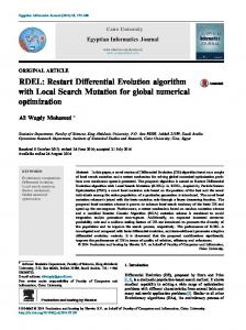
prespecified maximum number of FES when an algorithm is a success. Because the convergence graphs of the 30-D problems are similar to their 50-D and 100-D counterparts, they are given as represented here. Figure 1 illustrates the convergence characteristics of each algorithm for the four 30dimensional benchmark functions. From Table 5, we find that SapsDE almost achieves the fastest convergence speed at all functions, which is also displayed visually in Figure 1. Moreover, SapsDE obtains a higher success rate than the four DE variants in most instances. 4.5. Compared with ATPS. Recently, in [26], Zhu et al. proposed an adaptive population tuning scheme (ATPS) for DE. The ATPS adopts a dynamic population strategy to remove redundant individuals from the population according to its ranking order, perturb the population, and generate good
10
Mathematical Problems in Engineering Table 4: Experimental results of 100-dimensional problems 𝑓1 (𝑥)–𝑓17 (𝑥), averaged over 30 independent runs with 1 000 000 FES.
Function
DE
JADE
𝑗DE
SaDE
SapsDE
Mean error (std Dev)
Mean error (std Dev)
Mean error (std Dev)
Mean error (std Dev)
Mean error (std Dev)
1
1.21𝑒 − 39 (1.21𝑒 − 39)+ 6.89𝑒 − 189 (0.00𝑒 + 00)= 1.15𝑒 − 97 (1.34𝑒 − 97)+ 2.82𝑒 − 92 (1.48𝑒 − 91)+ 1.70e − 198 (0.00e + 00)
2
3.81𝑒 + 08 (1.57𝑒 + 08)+ 1.20𝑒 + 00 (1.86𝑒 + 00)+ 1.03𝑒 + 02 (4.06𝑒 + 01)+ 1.75𝑒 + 02 (7.03𝑒 + 01)+ 2.65e − 01 (1.01e + 00)
3
8.96𝑒 + 00 (7.84𝑒 − 01)+ 9.68𝑒 − 01 (5.18𝑒 − 01)+ 1.28e − 14 (3.70e − 15)= 2.92𝑒 + 00 (5.56𝑒 − 01)+
1.36𝑒 − 14 (2.07𝑒 − 15)
4
3.98𝑒 + 01 (9.40𝑒 + 00)+ 1.97𝑒 − 03 (4.21𝑒 − 03)= 0.00e + 00 (0.00e + 00)= 3.82𝑒 − 02 (5.92𝑒 − 02)+
1.07𝑒 − 03 (3.28𝑒 − 03)
5
8.52𝑒 + 02 (5.26𝑒 + 01)+
6
1.00𝑒 + 01 (7.87𝑒 − 01)+ 7.23𝑒 − 01 (9.71𝑒 − 02)+ 3.67𝑒 − 01 (4.79𝑒 − 02)+ 1.46𝑒 + 00 (2.97𝑒 − 01)+ 2.96e − 01 (3.17e − 02)
7
5.57𝑒 + 05 (5.85𝑒 + 05)+ 3.73𝑒 − 02 (8.14𝑒 − 02)= 1.04e − 03 (5.68e − 03)= 4.36𝑒 − 02 (1.12𝑒 − 01)=
8
3.69𝑒 + 06 (2.40𝑒 + 06)+ 1.07𝑒 − 01 (4.05𝑒 − 01)= 1.01𝑒 − 01 (5.52𝑒 − 01)= 1.62𝑒 − 01 (6.86𝑒 − 01)= 1.34e − 32 (5.56e − 48)
9
3.71𝑒 + 03 (9.46𝑒 + 02)+ 1.05𝑒 − 29 (2.43𝑒 − 29)= 2.73𝑒 − 29 (6.31𝑒 − 29)= 1.68e − 30 (9.22e − 30)= 5.47𝑒 − 30 (1.68𝑒 − 29)
10
3.82𝑒 + 05 (2.72𝑒 + 04)+ 6.51e − 15 (1.25e − 14)= 3.04𝑒 + 01 (1.84𝑒 + 01)+ 1.15𝑒 + 02 (3.38𝑒 + 01)+
11
2.29𝑒 + 09 (3.39𝑒 + 08)+ 3.25𝑒 + 05 (1.42𝑒 + 05)+ 2.28𝑒 + 06 (6.14𝑒 + 05)+ 4.26𝑒 + 06 (9.98𝑒 + 05)+ 2.20e + 05 (8.44e + 04)
12
4.47𝑒 + 05 (3.67𝑒 + 04)+ 7.80e + 03 (3.46e + 03)= 2.69𝑒 + 04 (9.63𝑒 + 03)+ 4.83𝑒 + 04 (1.06𝑒 + 04)+
8.59𝑒 + 03 (4.50𝑒 + 03)
13
2.40𝑒 + 08 (8.93𝑒 + 07)+ 1.20e + 00 (1.86e + 00)= 9.59𝑒 + 01 (4.48𝑒 + 01)+ 1.73𝑒 + 02 (4.20𝑒 + 01)+
1.72𝑒 + 00 (2.00𝑒 + 00)
14
2.13𝑒 + 01 (2.27𝑒 − 02)+ 2.13𝑒 + 01 (8.41𝑒 − 02)+ 2.13𝑒 + 01 (2.47𝑒 − 02)+ 2.13𝑒 + 01 (2.12𝑒 − 02)+ 2.03e + 01 (4.56e − 01)
15
8.58𝑒 + 02 (5.87𝑒 + 01)+ 1.78𝑒 − 16 (5.42𝑒 − 16)= 0.00e + 00 (0.00e + 00) 2.57𝑒 + 01 (7.00𝑒 + 00)+ 0.00e + 00 (0.00e + 00)
16
1.09𝑒 + 03 (3.06𝑒 + 01)+ 1.55𝑒 + 02 (3.51𝑒 + 01)+ 2.05𝑒 + 02 (2.94𝑒 + 01)+ 4.36𝑒 + 02 (6.18𝑒 + 01)+ 4.80e + 01 (9.04e + 00)
17
1.60𝑒 + 02 (1.70𝑒 + 00)+ 1.14𝑒 + 02 (9.12𝑒 + 00)+ 1.27𝑒 + 02 (3.55𝑒 + 00)+ 1.05𝑒 + 02 (7.30𝑒 + 00)+ 5.22e + 01 (2.21e + 00)
0.00e + 00 (0.00e + 00)
0.00e + 00 (0.00e + 00) 9.95𝑒 + 00 (2.75𝑒 + 00)+ 0.00e + 00 (0.00e + 00)
1.24𝑒 − 02 (3.70𝑒 − 02)
8.18𝑒 − 15 (1.63𝑒 − 14)
Total score
DE
JADE
𝑗DE
SaDE
SapsDE
+
17
7
10
14
∗
−
0
0
0
0
∗
=
0
10
7
3
∗
individuals. this APTS framework could be incorporated into several recently reported DE variants and achieves good performance on function optimization. In this section, we compare the SapsDE with the ATPS-DE variants, which are reported in [26], on nine 30-D benchmark functions. The parameter settings are the same as those in [26]. The averaged results of 30 independent runs are shown in the Table 6 (results for ATPS-DEs are taken from [26]). Obviously, from Table 6, we can observe that the number of “+” is more than that of “−”. On the whole, the SapsDE outperforms the ATPSDEs, respectively. 4.6. Time Complexity of SapsDE. In this section, we analyze time complexity of the SapsDE algorithm by using power regression 𝑦 = 𝑎𝑡𝑏 . Here 𝑡 is dimension 𝐷, and 𝑦 is the time in Table 7. Table 7 lists all time of the function with 30,
50, and 100 dimensions in 30 runs. After calculations, the results of power regression are also listed in Table 7. It can be found that the time complexity of our algorithm is less than 𝑂(𝐷2 ). 4.7. Parameter Study. In this section, we use 30-D test functions 𝑓1 –𝑓17 to investigate the impact of the initial 𝑁𝑃 value on SapsDE algorithm. The SapsDE algorithm runs 30 times on each function with three different initial 𝑁𝑃 values of 50, 100, and 200. We here present the results of mean and standard deviation for these functions in Table 8. Furthermore, we study the robustness of 𝑠 value by testing the 30-D benchmark functions 𝑓1 –𝑓17 . Similarly, the SapsDE algorithm runs 30 times on each function with three different 𝑠 values of 1, 3, and 5. The result of experiments is shown in Table 9.
Mathematical Problems in Engineering
11
Table 5: Experiment results of convergence speed and success rate. SapsDE
JADE
Sr
NFE
DE
Sr
NFE
𝑗DE
Sr
NFE
Sr
NFE
SaDE
Sr
NFE
𝐷 = 30 𝑓2
99641
96.67%
131700
93.33%
—
0%
—
0%
—
0%
𝑓3
42162
100%
73600
100%
256200
100%
143700
100%
66250
86.70%
𝑓10
98897
100%
103800
100%
—
0%
—
0%
—
0%
𝑓15
83882
100%
171200
100%
—
0%
138700
100%
83800
86.70%
𝑓2
174475
100%
267000
87%
—
0%
—
0%
—
0%
𝑓3
57610
100%
91800
100%
—
0%
206800
100%
348200
10%
𝑓10
232765
100%
275400
100%
—
0%
—
0%
—
0%
𝑓15
131032
100%
281700
100%
—
0%
217400
100%
149100
6.67%
𝐷 = 50
𝐷 = 100 𝑓2
629805
93.30%
802900
70%
—
0%
—
0%
—
0%
𝑓3
765400
3.33%
—
0%
—
0%
543700
13.30%
—
0%
𝑓10
946216
76.70%
977200
83.30%
—
0%
—
0%
—
0%
𝑓15
209975
100%
424600
100%
—
0%
382200
100%
—
0%
Table 6: Experimental results of SapsDE and ATPS-DEs. 𝑗DE-APTS
CoDE-APTS
JADE-APTS
SapsDE
Mean error (std Dev)
Mean error (std Dev)
Mean error (std Dev)
Mean error (std Dev)
9
0.00e + 00 (0.00e + 00)
8.82𝑒 − 17 (7.06𝑒 − 16)+
0.00e + 00 (0.00e + 00)
0.00e + 00 (0.00e + 00)
10
7.93𝑒 − 11 (2.31𝑒 − 11)+
2.70𝑒 − 03 (6.73𝑒 − 03)+
2.10e − 29 (4.86e − 29)−
1.17𝑒 − 28 (1.07𝑒 − 28)
11
9.83𝑒 + 04 (4.42𝑒 + 04)+
1.06𝑒 + 05 (8.03𝑒 + 05)+
7.43𝑒 + 03 (6.04𝑒 + 03)=
7.00e + 03 (4.29e + 03)
12
9.17𝑒 − 02 (8.02𝑒 − 02)+
1.55𝑒 − 03 (3.98𝑒 − 02)=
1.79e − 23 (9.76e − 23)=
4.22𝑒 − 15 (1.25𝑒 − 14)
13
3.87e − 01 (7.22e − 01)=
6.12𝑒 + 00 (4.39𝑒 + 00)+
8.59𝑒 + 00 (3.08𝑒 + 01)+
1.49𝑒 + 00 (5.68𝑒 + 00)
14
2.09𝑒 + 01 (1.09𝑒 − 02)+
2.07e + 01 (2.44e − 01)+
2.09𝑒 + 01 (6.43𝑒 − 02)+
2.07e + 01 (3.98e − 01)
Function
15
0.00e + 00 (0.00e + 00)
5.01𝑒 − 01 (3.40𝑒 − 01)+
5.42𝑒 − 12 (2.24𝑒 − 12)+
0.00e + 00 (0.00e + 00)
16
5.59𝑒 + 01 (2.47𝑒 + 01)+
5.10𝑒 + 01 (1.55𝑒 + 01)+
3.94𝑒 + 01 (1.16𝑒 + 01)+
2.18e + 01 (3.58e + 00)
17
7.90e + 00 (6.99e + 00)−
1.22𝑒 + 01 (6.30𝑒 + 00)−
2.19𝑒 + 01 (2.84𝑒 + 00)−
2.42𝑒 + 01 (1.68𝑒 + 00)
𝑗DE-APTS
CoDE-APTS
JADE-APTS
SapsDE
+
5
7
4
∗
−
1
1
2
∗
=
3
1
3
∗
Total score
From Tables 8 and 9, we find that SapsDE algorithm obtains similar optimization solutions on most of the functions by using three different initial 𝑁𝑃 values and 𝑠 values, respectively. Therefore, the performance of SapsDE algorithm is less sensitive to the parameter 𝑁𝑃 initial value between 50 and 200 and 𝑠 value between 1 and 5.
5. Conclusion This paper presents a SapsDE algorithm which utilizes two DE strategies and three novel population size adjustment strategies. As evolution processes, the algorithm selects a more suitable mutation strategy. Meanwhile, three popula-
12
Mathematical Problems in Engineering Table 7: Time complexity of SapsDE.
𝐷
𝑓1
𝑓2
𝑓3
𝑓4
𝑓5
𝑓6
𝑓7
𝑓8
𝑓9
30
112.163
112.1049
99.51729
119.3885
109.8877
98.08094
128.1295
129.8256
105.0963
50
250.8682
214.8441
194.698
229.0735
220.8529
192.6483
264.1902
269.5691
210.9053
100
763.8241
733.7201
736.4833
827.2118
735.0107
651.3032
942.6226
947.4914
688.3214
𝑎
4.94𝐸 − 01
0.504
0.30967
0.45001
0.47659
0.42848
0.42052
0.43884
0.48612
𝑏
1.5941
1.5726
1.6773
1.6219
1.5874
1.5831
1.6678
1.6603
1.5694
rss
6.0578
1391.343
1925.493
2275.271
772.9743
842.2943
1561.575
1335.442
596.6701
𝐷
𝑓10
𝑓11
𝑓12
𝑓13
𝑓14
𝑓15
𝑓16
𝑓17
30
132.4887
133.8268
141.0859
129.3506
140.4079
125.1071
136.9139
2292.366
50
303.5054
290.2551
270.1778
249.1615
302.0771
246.1471
295.1372
6133.686
100
1263.261
857.5675
1233.553
696.3027
914.3774
682.6456
879.7776
23393.98
𝑎
0.20834
0.69751
0.25784
1.0708
0.6923
1.0071
0.70463
3.2359
𝑏
1.8836
1.554
1.8234
1.403
1.5587
1.4129
1.5469
1.9295
2740.002
18.8848
11110.21
234.2553
90.6071
122.6194
45.898
110.6387
rss
Table 8: Robustness of 𝑁𝑃 value. 𝑁𝑃 = 50
𝑁𝑃 = 100
𝑁𝑃 = 200
Mean error (Std Dev)
Mean error (Std Dev)
Mean error (Std Dev)
1
4.38𝑒 − 126 (2.27𝑒 − 125)
9.59𝑒 − 126 (4.64𝑒 − 125)
3.32𝑒 − 120 (1.24𝑒 − 119)
2
1.32𝑒 − 01 (7.27𝑒 − 01)
1.32𝑒 − 01 (7.27𝑒 − 01)
6.64𝑒 − 01 (1.51𝑒 + 00)
3
2.66𝑒 − 15 (0.00𝑒 + 00)
2.66𝑒 − 15 (0.00𝑒 + 00)
2.66𝑒 − 15 (0.00𝑒 + 00)
4
0.00𝑒 + 00 (0.00𝑒 + 00)
0.00𝑒 + 00 (0.00𝑒 + 00)
0.00𝑒 + 00 (0.00𝑒 + 00)
5
0.00𝑒 + 00 (0.00𝑒 + 00)
0.00𝑒 + 00 (0.00𝑒 + 00)
0.00𝑒 + 00 (0.00𝑒 + 00)
6
1.77𝑒 − 01 (3.94𝑒 − 02)
1.78𝑒 − 01 (4.01𝑒 − 02)
1.83𝑒 − 01 (3.38𝑒 − 02)
7
1.57𝑒 − 32 (5.56𝑒 − 48)
1.57𝑒 − 32 (5.56𝑒 − 48)
1.57𝑒 − 32 (5.56𝑒 − 32)
8
1.34𝑒 − 32 (5.56𝑒 − 48)
1.34𝑒 − 32 (5.56𝑒 − 48)
1.34𝑒 − 32 (5.56𝑒 − 48)
9
0.00𝑒 + 00 (0.00𝑒 + 00)
0.00𝑒 + 00 (0.00𝑒 + 00)
0.00𝑒 + 00 (0.00𝑒 + 00)
10
1.17𝑒 − 28 (1.07𝑒 − 28)
9.85𝑒 − 29 (9.93𝑒 − 29)
9.19𝑒 − 29 (1.00𝑒 − 28)
11
7.00𝑒 + 03 (4.29𝑒 + 03)
7.02𝑒 + 03 (5.74𝑒 + 03)
7.16𝑒 + 03 (5.09𝑒 + 03)
12
4.22𝑒 − 15 (1.25𝑒 − 14)
6.17𝑒 − 14 (2.32𝑒 − 13)
5.16𝑒 − 15 (1.37𝑒 − 14)
13
1.49𝑒 + 00 (5.68𝑒 + 00)
2.65𝑒 + 00 (7.29𝑒 + 00)
1.64𝑒 + 00 (5.76𝑒 + 00)
14
2.07𝑒 + 01 (3.98𝑒 − 01)
2.07𝑒 + 01 (3.74𝑒 − 01)
2.08𝑒 + 01 (3.19𝑒 − 01)
15
0.00𝑒 + 00 (0.00𝑒 + 00)
0.00𝑒 + 00 (0.00𝑒 + 00)
0.00𝑒 + 00 (0.00𝑒 + 00)
16
2.18𝑒 + 01 (3.58𝑒 + 00)
2.11𝑒 + 01 (4.28𝑒 + 00)
2.33𝑒 + 01 (4.82𝑒 + 00)
17
2.42𝑒 + 01 (1.68𝑒 + 00)
2.41𝑒 + 01 (1.95𝑒 + 00)
2.41𝑒 + 01 (2.34𝑒 + 00)
Function
tion size adjustment strategies will dynamically tune the 𝑁𝑃 value according to the improvement status learned from the previous generations. We have investigated the characteristics of SapsDE. Experiments show that SapsDE has low time complexity, fast convergence, and high success rate. The sensitivity analysis of initial 𝑁𝑃 value and 𝑠 indicates that
they have insignificant impact on the performance of the SapsDE. We have compared the performance of SapsDE with the classic DE and four adaptive DE variants over a set of benchmark functions chosen from the existing literature and CEC 2005 special session on real-parameter optimization
Mathematical Problems in Engineering
13 Table 9: Robustness of 𝑠 value.
𝑠=1 Mean error (Std Dev)
𝑠=3 Mean error (Std Dev)
𝑠=5 Mean error (Std Dev)
1 2
4.38𝑒 − 126 (2.27𝑒 − 125) 1.32𝑒 − 01 (7.27𝑒 − 01)
6.67𝑒 − 119 (3.65𝑒 − 118) 3.98𝑒 − 01 (1.21𝑒 + 00)
3.84𝑒 − 143 (1.57𝑒 − 142) 6.64𝑒 − 01 (1.51𝑒 + 00)
3 4
2.66𝑒 − 15 (0.00𝑒 + 00) 0.00𝑒 + 00 (0.00𝑒 + 00)
3.01𝑒 − 15 (1.08𝑒 − 15) 1.47𝑒 − 3 (3.46𝑒 − 03)
2.78𝑒 − 15 (6.48𝑒 − 16) 1.56𝑒 − 03 (4.45𝑒 − 03)
5 6 7
0.00𝑒 + 00 (0.00𝑒 + 00) 1.77𝑒 − 01 (3.94𝑒 − 02) 1.57𝑒 − 32 (5.56𝑒 − 48)
0.00𝑒 + 00 (0.00𝑒 + 00) 1.96𝑒 − 01 (1.82𝑒 − 02) 1.57𝑒 − 32 (5.56𝑒 − 48)
0.00𝑒 + 00 (0.00𝑒 + 00) 1.96𝑒 − 01 (1.82𝑒 − 02) 1.57𝑒 − 32 (5.56𝑒 − 48)
8 9
1.34𝑒 − 32 (5.56𝑒 − 48) 0.00𝑒 + 00 (0.00𝑒 + 00)
1.34𝑒 − 32 (5.56𝑒 − 48) 0.00𝑒 + 00 (0.00𝑒 + 00)
1.34𝑒 − 32 (5.56𝑒 − 48) 0.00𝑒 + 00 (0.00𝑒 + 00)
10 11 12
1.17𝑒 − 28 (1.07𝑒 − 28) 7.00𝑒 + 03 (4.29𝑒 + 03) 4.22𝑒 − 15 (1.25𝑒 − 14)
5.08𝑒 − 28 (2.51𝑒 − 28) 5.19𝑒 + 03 (4.64𝑒 + 03) 1.03𝑒 − 06 (2.14𝑒 − 06)
6.92𝑒 − 28 (5.60𝑒 − 28) 5.09𝑒 + 03 (3.17𝑒 + 03) 1.07𝑒 − 06 (3.07𝑒 − 06)
13 14
1.49𝑒 + 00 (5.68𝑒 + 00) 2.07𝑒 + 01 (3.98𝑒 − 01)
3.04𝑒 + 00 (1.22𝑒 + 01) 2.05𝑒 + 01 (4.07𝑒 − 01)
5.31𝑒 − 01 (1.37𝑒 + 00) 2.06𝑒 + 01 (3.24𝑒 − 01)
15 16 17
0.00𝑒 + 00 (0.00𝑒 + 00) 2.18𝑒 + 01 (3.58𝑒 + 00) 2.42𝑒 + 01 (1.68𝑒 + 00)
0.00𝑒 + 00 (0.00𝑒 + 00) 3.16𝑒 + 01 (6.60𝑒 + 00) 1.91𝑒 + 01 (4.04𝑒 + 00)
0.00𝑒 + 00 (0.00𝑒 + 00) 3.34𝑒 + 01 (7.00𝑒 + 00) 1.81𝑒 + 01 (4.14𝑒 + 00)
1020
105
1010
100
10
Mean error
Mean error: 𝑓(𝑥) − 𝑓(𝑥∗ )
Function
0
10−10 10−20 10−30
0
0.5
1
1.5
2
2.5
3
FES
10−5 10−10 10−15
3.5 ×10⁵
0
0.5
1
1.5
(a)
10
100 10−10 10−20 10−30
0
0.5
1
1.5
2 FES
2.5
3
3.5 ×10⁵
𝑗DE SaDE
SapsDE DE JADE
2.5
3
3.5 ×10⁵
(b)
10
Mean error
Mean error
10
2 FES
(c)
5
100 10−5 10−10 10−15
0
0.5
1
1.5
2
2.5
FES
3 ×10⁵
𝑗DE SaDE
SapsDE DE JADE (d)
Figure 1: Performance of the algorithms for two 30-dimensional benchmark functions—(a) 𝑓2 ; (b) 𝑓3 ; (c) 𝑓10 ; (d) 𝑓15 .
problems, and we conclude that the SapsDE algorithm is a highly competitive algorithm in 30-, 50-, and 100dimensional problems. To summarize the results of the tests, the SapsDE algorithm presents significantly better results
than the remaining algorithms in most cases. In our future work, we will focus on solving some real-world problems with the SapsDE. We will also tend to modify it for discrete problems.
14
Mathematical Problems in Engineering
Acknowledgment This paper was partially supported by the National Natural Science Foundation of China (61271114).
[16]
References [1] Y. Tang, H. Gao, J. Kurths, and J. Fang, “Evolutionary pinning control and its application in UAV coordination,” IEEE Transactions on Industrial Informatics, vol. 8, pp. 828–838, 2012. [2] A. Tuson and P. Ross, “Adapting operator settings in genetic algorithms,” Evolutionary Computation, vol. 6, no. 2, pp. 161–184, 1998. [3] Y. Tang, Z. Wang, H. Gao, S. Swift, and J. Kurths, “A constrained evolutioanry computation method for detecting controlling regions of cortical networks,” IEEE/ACM Transactions on Computational Biology and Bioinformatics, vol. 9, pp. 1569–1581, 2012. [4] J. Kennedy and R. Eberhart, “Particle swarm optimization,” in Proceedings of the IEEE International Conference on Neural Networks, pp. 1942–1948, December 1995. [5] Y. Tang, Z. Wang, and J. A. Fang, “Controller design for synchronization of an array of delayed neural networks using a controllable probabilistic PSO,” Information Sciences, vol. 181, no. 20, pp. 4715–4732, 2011. [6] R. Storn and K. Price, “Differential evolution—a simple and efficient heuristic for global optimization over continuous spaces,” Journal of Global Optimization, vol. 11, no. 4, pp. 341– 359, 1997. [7] Y. Tang, H. Gao, W. Zou, and J. Kurths, “Identifying controlling nodes in neuronal networks in different scales,” PLoS ONE, vol. 7, Article ID e41375, 2012. [8] J. Gomez, D. Dasgupta, and F. Gonzalez, “Using adaptive operators in genetic search,” in Proceedings of the Genetic and Evolutionary Computing Conference, pp. 1580–1581, Chicago, Ill, USA, July 2003. [9] S. Das and S. Sil, “Kernel-induced fuzzy clustering of image pixels with an improved differential evolution algorithm,” Information Sciences, vol. 180, no. 8, pp. 1237–1256, 2010. [10] S. Das, A. Abraham, and A. Konar, “Automatic clustering using an improved differential evolution algorithm,” IEEE Transactions on Systems, Man, and Cybernetics Part A, vol. 38, no. 1, pp. 218–237, 2008. [11] Y. Tang, Z. Wang, and J. Fang, “Feedback learning particle swarm optimization,” Applied Soft Computing, vol. 11, pp. 4713– 4725, 2011. [12] J. Zhang and A. C. Sanderson, “An approximate Gaussian model of differential evolution with spherical fitness functions,” in Proceedings of the IEEE Congress on Evolutionary Computation (CEC ’07), pp. 2220–2228, Singapore, September 2007. [13] K. V. Prie, “An introduction to differential evolution,” in New Ideas in Oprimization, D. Corne, M. Dorigo, and F. Glover, Eds., pp. 79–108, McGraw-Hill, London, UK, 1999. [14] V. L. Huang, A. K. Qin, and P. N. Suganthan, “Self-adaptive differential evolution algorithm for constrained real-parameter optimization,” in Proceedings of the IEEE Congress on Evolutionary Computation (CEC ’06), pp. 17–24, Vancouver, Canada, July 2006. [15] J. Brest, S. Greiner, B. Boˇskovi´c, M. Mernik, and V. Zumer, “Self-adapting control parameters in differential evolution: a comparative study on numerical benchmark problems,” IEEE
[17]
[18]
[19]
[20]
[21]
[22]
[23]
[24]
[25]
[26]
[27]
[28]
[29]
[30]
[31]
Transactions on Evolutionary Computation, vol. 10, no. 6, pp. 646–657, 2006. ˇ J. Brest, V. Zumer, and M. S. Mauˇcec, “Self-adaptive differential evolution algorithm in constrained real-parameter optimization,” in Proceedings of the IEEE Congress on Evolutionary Computation (CEC ’06), pp. 215–222, Vancouver, Canada, July 2006. ˇ and M. S. Mauˇcec, J. Brest, B. Boˇskov´c, S. Greiner, V. Zumer, “Performance comparison of self-adaptive and adaptive differential evolution algorithms,” Soft Computing, vol. 11, no. 7, pp. 617–629, 2007. J. Teo, “Exploring dynamic self-adaptive populations in differential evolution,” Soft Computing, vol. 10, no. 8, pp. 673–686, 2006. Z. Yang, K. Tang, and X. Yao, “Self-adaptive differential evolution with neighborhood search,” in Proceedings of the IEEE Congress on Evolutionary Computation (CEC ’08), pp. 1110–1116, Hong Kong, June 2008. A. K. Qin and P. N. Suganthan, “Self-adaptive differential evolution algorithm for numerical optimization,” in Proceedings of the IEEE Congress on Evolutionary Computation (IEEE CEC ’05), pp. 1785–1791, Edinburgh, UK, September 2005. A. K. Qin, V. L. Huang, and P. N. Suganthan, “Differential evolution algorithm with strategy adaptation for global numerical optimization,” IEEE Transactions on Evolutionary Computation, vol. 13, no. 2, pp. 398–417, 2009. R. S. Rahnamayan, H. R. Tizhoosh, and M. M. A. Salama, “Opposition-based differential evolution,” IEEE Transactions on Evolutionary Computation, vol. 12, no. 1, pp. 64–79, 2008. N. Noman and H. Iba, “Accelerating differential evolution using an adaptive local search,” IEEE Transactions on Evolutionary Computation, vol. 12, no. 1, pp. 107–125, 2008. T. B¨ack, A. E. Eiben, and N. A. L. van der Vaart, “An empirical study on GAs ”without parameters”,” in Proceedings of the 6th Conference on Parallel Problem Solving from Nature, M. Schoenauer, K. Deb, G. Rudolph et al., Eds., vol. 1917 of Lecture Notes in Computer Science, pp. 315–324, Springer, Berlin, Germany, 2000. W. Zhu, J.-A. Fang, Y. Tang, W. Zhang, and W. Du, “Digital IIR filters design using differential evolution algorithm with a controllable probabilistic population size,” PLoS ONE, vol. 7, Article ID e40549, 2012. W. Zhu, Y. Tang, J.-A. Fang, and W. Zhang, “Adaptive population tuning scheme for differential evolution,” Information Sciences, vol. 223, pp. 164–191, 2013. J. Zhang and A. C. Sanderson, “JADE: adaptive differential evolution with optional external archive,” IEEE Transactions on Evolutionary Computation, vol. 13, no. 5, pp. 945–958, 2009. P. N. Suganthan, N. Hansen, J. J. Liang et al., “Problem definitions and evaluation criteria for the CEC 2005 special session on real-parameter optimization,” KanGAL Report, Nanyang Technological University, Singapore; IIT Kanpur, Kanpur, India, 2005. X. Yao, Y. Liu, and G. Lin, “Evolutionary programming made faster,” IEEE Transactions on Evolutionary Computation, vol. 3, no. 2, pp. 82–102, 1999. K. V. Price, R. M. Storn, and J. A. Lampinen, Differential Evolution: A Practical Approach to Global Optimization, Springer, Berlin, Germany, 2005. N. Noman and H. Iba, “Accelerating differential evolution using an adaptive local search,” IEEE Transactions on Evolutionary Computation, vol. 12, no. 1, pp. 107–125, 2008.
Advances in
Operations Research Hindawi Publishing Corporation http://www.hindawi.com
Volume 2014
Advances in
Decision Sciences Hindawi Publishing Corporation http://www.hindawi.com
Volume 2014
Journal of
Applied Mathematics
Algebra
Hindawi Publishing Corporation http://www.hindawi.com
Hindawi Publishing Corporation http://www.hindawi.com
Volume 2014
Journal of
Probability and Statistics Volume 2014
The Scientific World Journal Hindawi Publishing Corporation http://www.hindawi.com
Hindawi Publishing Corporation http://www.hindawi.com
Volume 2014
International Journal of
Differential Equations Hindawi Publishing Corporation http://www.hindawi.com
Volume 2014
Volume 2014
Submit your manuscripts at http://www.hindawi.com International Journal of
Advances in
Combinatorics Hindawi Publishing Corporation http://www.hindawi.com
Mathematical Physics Hindawi Publishing Corporation http://www.hindawi.com
Volume 2014
Journal of
Complex Analysis Hindawi Publishing Corporation http://www.hindawi.com
Volume 2014
International Journal of Mathematics and Mathematical Sciences
Mathematical Problems in Engineering
Journal of
Mathematics Hindawi Publishing Corporation http://www.hindawi.com
Volume 2014
Hindawi Publishing Corporation http://www.hindawi.com
Volume 2014
Volume 2014
Hindawi Publishing Corporation http://www.hindawi.com
Volume 2014
Discrete Mathematics
Journal of
Volume 2014
Hindawi Publishing Corporation http://www.hindawi.com
Discrete Dynamics in Nature and Society
Journal of
Function Spaces Hindawi Publishing Corporation http://www.hindawi.com
Abstract and Applied Analysis
Volume 2014
Hindawi Publishing Corporation http://www.hindawi.com
Volume 2014
Hindawi Publishing Corporation http://www.hindawi.com
Volume 2014
International Journal of
Journal of
Stochastic Analysis
Optimization
Hindawi Publishing Corporation http://www.hindawi.com
Hindawi Publishing Corporation http://www.hindawi.com
Volume 2014
Volume 2014