Differential Evolution for Multi-Objective Optimization B.V.Babu*
M. Mathew Leenus Jehan
Assistant Dean - ESD & Head - Chemical Engineering & Engg. Tech. Depts. B.I.T.S., PILANI 333 031 (India)
[email protected]
Chemical Engineering Department B.I.T.S. Pilani PILANI 333 031 (India)
[email protected]
Abstract- Two test problems on Multi-objective optimization (one simple general problem and the second one on an engineering application of cantilever design problem) are solved using Differential Evolution (DE). DE is a population based search algorithm, which is an improved version of Genetic Algorithm (GA), Simulations carried out involved solving (1) both the problems using Penalty function method, and (2) first problem using Weighing factor method and finding Pareto optimum set for the chosen problem, DE found to be robust and faster in optimization. To consolidate the power of DE, the classical Himmelblau function, with bounds on variables, is also solved using both DE and GA. DE found to give the exact optimum value within less generations compared to simple GA.
to their population-based search approach. Thus, EAs are ideally suited for multi-objective optimization problems. A detailed account of multi-objective optimization using evolutionary algorithms and some of the applications using genetic algorithms can be found in literature (Deb, 2001; Rajesh et al., 2000; Rajesh et al., 2001; Oh et al., 2002).
1 Introduction Optimization is a procedure of finding and comparing feasible solutions until no better solution can be found. Solutions are termed good or bad in terms of an objective, which is often the cost of fabrication, amount of harmful gases, efficiency of a process, product reliability, or other factors (Deb, 2001). Most of the real world problems involve more than one objective, making the multiple conflicting objectives interesting to solve. Classical optimization methods are inconvenient to solve multiobjective optimization problems, as they could at best find one solution in one simulation run. As the real world problems involve the simulation and optimization of multiple objectives, results and solutions of these problems are conceptually different from single objective function problems. In multiobjective optimization, there may not exist a solution that is best with respect to all objectives. Instead, there are equally good, which are known as pareto optimal solutions. A pareto optimal set of solution is such that when we go from any one point to another in the set, atleast one objective function improves and at least one other worsen (Yee et al., 2003). Neither of the solution dominates over each other and all the sets of decision variables on the pareto are equally good. However, Evolutionary algorithms (EAs) can find multiple optimal solutions in one single simulation run due
2 Differential Evolution (DE) Differential Evolution (Price and Storn, 1997) is an improved version of Genetic Algorithm (Goldberg, 1989) for faster optimization. Genetic algorithm (GA) is a search technique developed by Holland (1975) which mimics the principle of natural evolution. In this technique (simple GA), the decision variables is first decoded into binary numbers [0 and 1] and hence creat a population pool. Each of these vectors or chromosomes generally called is then mapped into its real value using specified lower and upper bounds. A model of the process will then compute an objective function for each chromosome and then give the fitness of the chromosome. The optimization search proceeds through three operators: reproduction, crossover and mutation. The reproduction (selection) operator selects good strings in a population and forms mating pool. The chromosomes are copied based on their fitness value. No new strings are produces in this operation. The crossover allows for a new string formation by exchanging some portion of the strings (chosen randomly) with string of another chromosome generating child chromosome in the mating pool. If the child chromosome are less fit than the parent chromosome, the will slowly die in the subsequent generation. The effect of crossover can be detrimental or good. Hence, not all the strings are used for crossover. A crossover probability, pc is used, where only 100 pc percent of the strings in the mating pool are involved in crossover operation while the rest continue unchanged to the next generation. Mutation is the last operation. It is used to further perturb the child vector using mutation probability pm. The mutation alters the string locally to create a better string. Mutation is needed to create a point in the neighborhood of the current point, thereby achieving a local search and maintaining the diversity in the population. The entire process is repeated till some
termination criterion is met. A detailed description of GA is documented in Holland (1975) and Goldberg (1989). Unlike simple GA that uses binary coding for representing problem parameters, Differential Evolution (DE) uses real coding of floating point numbers. Among the DE’s advantages are its simple structure, ease of use, speed and robustness. The simple adaptive scheme used by DE ensures that these mutation increments are automatically scaled to the correct magnitude. Similarly DE uses a non-uniform crossover in that the parameter values of the child vector are inherited in unequal proportions from the parent vectors. For reproduction, DE uses a tournament selection where the child vector competes against one of its parents. The overall structure of the DE algorithm resembles that of most other population based searches. The parallel version of DE maintains two arrays, each of which holds a population of NP, D-dimensional, real valued vectors. The primary array holds the current vector population, while the secondary array accumulates vectors that are selected for the next generation. In each generation, NP competitions are held to determine the composition of the next generation. Every pair of vectors (Xa, Xb) defines a vector differential: Xa - Xb. When Xa and Xb are chosen randomly, their weighted differential is used to perturb another randomly chosen vector Xc. This process can be mathematically written as X’c = Xc + F(Xa-Xb). The scaling factor F is a user supplied constant in the range (0 < F ≤ 1.2). The optimal value of F for most of the functions lies in the range of 0.4 to 1.0 (Price & Storn, 1997). Then in every generation, each primary array vector, Xi is targeted for crossover with a vector like X’c to produce a trial vector Xt. Thus the trial vector is the child of two parents, a noisy random vector and the target vector against which it must compete. The non-uniform crossover is used with a crossover constant CR, in the range 0 ≤ CR ≤1. CR actually represents the probability that the child vector inherits the parameter values from the noisy random vector. When CR = 1, for example, every trial vector parameter is certain to come from X’c. If, on the other hand, CR = 0, all but one trial vector parameter comes from the target vector. To ensure that Xt differs from Xi by at least one parameter, the final trial vector parameter always comes from the noisy random vector, even when CR = 0. Then the cost of the trial vector is compared with that of the target vector, and the vector that has the lowest cost of the two would survive for the next generation. In all, just three factors control evolution under DE, the population size, NP; the weight applied to the random differential, F; and the crossover constant, CR. 2.1 Different strategies of DE Different strategies can be adopted in DE algorithm depending upon the type of problem for which DE is applied. The strategies can vary based on the vector to be perturbed, number of difference vectors considered for perturbation, and finally the type of crossover used. The
following are the ten different working strategies proposed by Price & Storn (2003): 1. DE/best/1/exp 2. DE/rand/1/exp 3. DE/rand-to-best/1/exp 4. DE/best/2/exp 5. DE/rand/2/exp 6. DE/best/1/bin 7. DE/rand/1/bin 8. DE/rand-to-best/1/bin 9. DE/best/2/bin 10. DE/rand/2/bin The general convention used above is DE/x/y/z. DE stands for Differential Evolution, x represents a string denoting the vector to be perturbed, y is the number of difference vectors considered for perturbation of x, and z stands for the type of crossover being used (exp: exponential; bin: binomial). Thus, the working algorithm outlined above is the seventh strategy of DE i.e. DE/rand/1/bin. Hence the perturbation can be either in the best vector of the previous generation or in any randomly chosen vector. Similarly for perturbation either single or two vector differences can be used. For perturbation with a single vector difference, out of the three distinct randomly chosen vectors, the weighted vector differential of any two vectors is added to the third one. Similarly for perturbation with two vector differences, five distinct vectors, other than the target vector are chosen randomly from the current population. Out of these, the weighted vector difference of each pair of any four vectors is added to the fifth one for perturbation. In exponential crossover, the crossover is performed on the D variables in one loop until it is within the CR bound. The first time a randomly picked number between 0 and 1 goes beyond the CR value, no crossover is performed and the remaining D variables are left intact. In binomial crossover, the crossover is performed on each of the D variables whenever a randomly picked number between 0 and 1 is within the CR value. So for high values of CR, the exponential and binomial crossovers yield similar results. The strategy to be adopted for each problem is to be determined separately by trial and error. A strategy that works out to be the best for a given problem may not work well when applied for a different problem. Price & Storn (1997) gave the working principle of DE with single strategy. Later on, they suggested ten different strategies of DE (Price & Storn, 2003). A strategy that works out to be the best for a given problem may not work well when applied for a different problem. Also, the strategy and key parameters to be adopted for a problem are to be determined by trial & error. However, strategy-7 (DE/rand/1/bin) is the most successful and the most widely used strategy. The key parameters of control in DE are: NP-the population size, CR-the crossover constant, and F-the weight applied to random differential (scaling factor). Babu et al. (2002) proposed a new concept called ‘nested DE’ to automate the choice of DE key parameters. In addition, some new strategies have
been proposed and successfully applied to optimization of extraction process (Babu & Angira, 2003a). As detailed above, the crucial idea behind DE is a scheme for generating trial parameter vectors. Basically, DE adds the weighted difference between two population vectors to a third vector. Price & Storn (2003) have given some simple rules for choosing key parameters of DE for any given application. Normally, NP should be about 5 to 10 times the dimention (number of parameters in a vector) of the problem. As for F, it lies in the range 0.4 to 1.0. Initially F = 0.5 can be tried then F and/or NP is increased if the population converges prematurely. A good first choice for CR is 0.1, but in general CR should be as large as possible. DE has been successfully applied in various fields. Some of the successful applications of DE include: digital filter design (Storn, 1995), batch fermentation process (Chiou & Wang, 1999; Wang & Cheng, 1999), estimation of heat transfer parameters in trickle bed reactor (Babu & Sastry, 1999), optimal design of heat exchangers [Babu & Munawar, 2000; 2001), synthesis & optimization of heat integrated distillation system [Babu & Singh, 2000), optimization of an alkylation reaction [Babu & Gaurav, 2000), scenario-integrated optimization of dynamic systems (Babu & Gautam, 2001), optimization of nonlinear functions (Babu & Angira, 2001a), optimization of thermal cracker operation (Babu & Angira, 2001b), global optimization of MINLP problems (Babu & Angira, 2002a), optimization of non-linear chemical processes (Babu & Angira, 2002b), global optimization of nonlinear chemical engineering processes (Angira & Babu, 2003), optimization of water pumping system (Babu & Angira, 2003b), optimization of biomass pyrolysis (Babu & Chaurasia, 2003), etc. Many engineering applications using various evolutionary algorithms have been reported in literature (Dasgupta & Michalewicz, 1997; Onwubolu & Babu, 2003). DE applications on Multi-objective optimization are scarce (Abbass 2001; 2002). In this study, DE is applied to two test problems of multiobjective optimization and three test problmes of singleobjective optimization with bounds on variables. The results are compared with those obtained using GA.
•
•
•
•
•
•
•
3 Pseudo Code for DE The pseudo code of DE used in the present study is given below: • Choose a seed for the random number generator. • Initialize the values of D, NP, CR, F and MAXGEN (maximumgeneration). • Initialize all the vectors of the population randomly. The variable are normalized within the bounds. Hence generate a random number between 0 and 1 for all the design variables for initialization. for i = 1 to NP
•
•
{ for j = 1 to D Xi,j =Lower bound+ random number *( upper bound - lower bound)} All the vectors generated should satisfy the constraints. Penalty function approach, i.e., penalizing the vector by giving it a large value, is followed only for those vectors, which do not satisfy the constraints. Evaluate the cost of each vector. Profit here is the value of the objective function to be maximized calculated by a separate function defunct.profit() for i = 1 to NP Ci = defunct.profit() Find out the vector with the maximum profit i.e. the best vector so far. Cmax = C1 and best =1 for i = 2 to NP { if (Ci> Cmax) then Cmin = Ci and best = i } Perform mutation, crossover, selection and evaluation of the objective function for a specified number of generations. While (gen < MAXGEN) { for i = 1 to NP { For each vector Xi (target vector), select three distinct vectors Xa, Xb and Xc (select five, if two vector differences are to be used) randomly from the current population (primary array) other than the vector Xi do { r1 = random number * NP r2 = random number * NP r3 = random number * NP } while (r1=i)OR(r2=i)OR(r3=i)OR(r1=r2 )OR(r2=r3)OR(r1=r3) Perform crossover for each target vector Xi with its noisy vector Xn,i and create a trial vector, Xt,i. The noisy vector is created by performing mutation. If CR = 0 inherit all the parameters from the target vector Xi, except one which should be from Xn,i. for binomial crossover { p = random number for n = 1 to D {if ( p Ci ) new Xi = Xt,i else new Xi = Xi } /* for i=1 to NP */ } Print the results (after the stopping criteria is met).
The stopping criteria may be of two kinds. One may be some convergence criterion that states that the error in the minimum or maximum between two previous generations should be less than some specified value (standard deviation may be used). The other may be an upper bound on the number of generations. The stopping criteria may be a combination of the two as well. In the present study, test problem-1 is soloved uisng second critea, whereas the test problem-2 is solved using the first criteria.
4 Test Problem–1 solved using Penalty function This problem (Belegundu and Chandrupatla, 2002) has two objective functions. One objective function is used as a constraint. Single optimal solution is obtained after 40 iterations. Penalty Function Method (Deb, 2001; Belegundu and Chandrupatla, 2002) is implemented to handle the constraint using DE algorithm. 4.1 Problem Statement Maximize 3x1 + x2 + 1 Maximize –x1 + 2x2 Subject to 0 T x1 T 3,
0 T x2 T 3
4.2 Parameters Used Penalty parameter (r) = 4.0 Number of population points (NP) = 20 Number of Iterations = 40 DE Key Parameters: Scaling Factor (F) = 0.45 Cross-over Constant (CR) = 0.9 4.3 Simulation Results A single optimum is found after 40 iterations. x1 = 1.875 x2 = 3.0 4.4 Discussion In this problem second objective function is taken as a constraint and normalized as below: -x1 + 2x2 ≥ c -x1 + 2x2 – c ≥ 0. Normalizing constraints in the above manner has an additional advantage. Since all normalized constraint
violations take place more or less the same order of magnitude, they all can be simply added as the overall constraint violation and thus only one penalty parameter r will be needed to make the overall constraint violation, of the same order as the objective function. Here c is a constant set by the user. By changing the c value, we can get different single optimum solutions by this program. Here the value of c can take any value between 6 to 3 because the maximum and minimum value of second objective function is 6 and 3 as per maximizing first objective function. Then higher-level information is used to decide a single value of c to end up with a single optimal value of x1and x2. It is also important to note that for maximizing both objective functions, x2 value should take the maximum possible value (3.0). i.e, by changing any ‘c’ value we should end up with x2 value as 3.0.
5 Test Problem-1 solved using Weighing factor The above problem (Belegundu and Chandrupatla, 2002) is also solved using weighing factor method. The weighted sum method scalarizes a set of objective into a single objective by premultiplying each objective with a user supplies weight (Deb, 2001). This is the most widely used classical and simplest approach. The value of the weight depends on the importance of the each objective in the context of the problem. The weight of an objective is usually chosen in proportion to the objective’ s relative importance in the problem. Then a composite objective function can be formed by summing the weighted objective and the multiobjective optimization gives is then converted to a single objective optimization. It is a usual practice to choose weights such that therir sum is one. A set of pareto optimal solutions is obtained after 100 iterations. DE algorithm with Weighing Factor Method (Deb, 2001) is used for this work. 5.1 Problem Statement Maximize 3x1 + x2 + 1 Maximize –x1 + 2x2 Subject to 0 T x1 T 3,
0 T x2 T 3
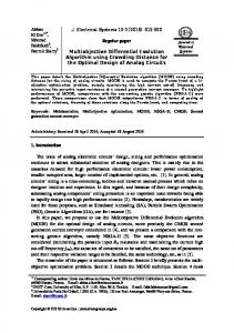
5.2 Parameters Used Weighing factors: w1 = 0.25; w2 = 0.75 Number of Population points (NP) = 20 Number of Iterations = 100 DE Key Parameters: Scaling Factor (F) = 0.45 Cross-over Constant (CR) = 0.9 5.3 Simulation Results A set of Pareto optimum solutions is obtained after 100 iterations using differential evolution algorithm. Computer code is developed in C++ for this work. It will give the graphical display of Pareto optimum solutions in each iteration.
5.4 Discussion The Penalty function method is simple and a single optimum is obtained, as one of the two objective functions has been considered as a constraint (second objective function in the present case). The convergence is obtained within 40 iterations.
subjet to σmax ≤ Sy, δ ≤ δmax
Pareto optimum set obtained after 100 iterations using DE
whereas the maximum stress is calculated as follows: σmax = 32Pl/(πd3) where, E = Young’ s Modulus, GPa
6
f2
4 2 0 0
5
10
is smaller than a specified limit δmax. With all of the above considerations, the following two–objective optimisation problem is formulated as follows: 2 Minimize f1(d,l) = ρπd l/4 3 4 Minimize f2(d,l) = δ = 64Pl /(3Eπd )
15
f1
Fig.3.2 Pareto optimum set obtained Weighing factor method, on the other hand, is popular and simplest way to solve a multi objective optimization, which gives a set of pareto optimum solutions. Though it took more iterations (100 iterations for the chosen problem in this study), the concept is intuitive and easy to use. For problems having a convex Pareto-optimal front, this method guarantees finding solutions on the entire Paretooptimal set (Deb, 2001). From those multiple optimal solutions, we can choose the good Pareto optimum set. In this study, first two weighing factors w1 and w2 are found using trail and error method. It is also found that any other combination of weighing factors end up with optimization of single objective function.
6 Test Problem-2 solved using Penalty function A cantilever design problem (Deb, 2001) with two decision variable, diameter (d) and length (l) is considered. The beam has to carry an end load P. Let us consider two conflicting objective of the design, i.e., minimization of weight f1 and minimization of end deflection f2. The first objective will resort to an optimum solution having the smaller dimensions of d and l, so that the overall weight of the beam is minimum. Since dimensions are small, the beam will not be adequately rigid and the end deflection of the beam will be large. On the other hand, if the beam is minimized for end deflection, the dimensions of the beam are expected to be large, thereby making the weight of the beam large. We consider two constraints for our discussion here. The developed maximum stress is less than the allowable strength (Sy) and the end deflection (δ)
The following parametric values are used: ρ = 7800 kg/m3 P = 1 kN E = 207 GPa Sy = 300 MPa δmax = 5 mm The upper and lower bounds for l and d are: 200 ≤ l ≤ 1000 mm 10 ≤ d ≤ 50 mm 6.1 Parameters Used Penalty parameter (r) = 1000.0 Number of population points (NP) = 20 Standard Deviation (σ ) = 0.0001 DE Key Parameters: Scaling Factor (F) = 0.6 Cross-over Constant (CR) = 0.85 6.2 Simulation Results A single optimum is found after 49 iterations. l = 200.14 mm d = 21.651 mm f1 = 0.577 kg f2 = 1.194 mm 6.3 Discussion In this problem also, the second objective function is taken as a constraint and normalized as below: 3 4 f2 = 64Pl /(3Eπd ) ≤ c f2/c – 1 ≤ 0 where c = 5 mm = maximum allowable deflection of the beam. The value of c has to defined by the user. The importance of normalizing the function has already been explained in section-4.4. As mentioned earlier, the first convergence criterion is being used as condition for termination. Because, it gives the exact generation number at which the convergence of all the population points to a single value occurs. Obviously, as there would be no betterment in terms of obtained global solution, it is needless to go for further iterations (generations). However, in the case of second criterion, which may be used for comparison purposes of various different algorithms, the iterations continue even if
it converged to a global optimum at the expense of computational time..
DE were obtained to be the same. This also proves DE’ s power and robustness.
7 Himmelblau Function
8 Conclusions
An objective function was taken and simulated using both Differential Evolution (DE) and Simple Genetic Algorithm (GA). In DE all points in the population converged and gave exact solution after 60 iterations. GA gives some good points after 100 generations.
In this study, DE, an improved version of GA, is used for solving two problems: (1) a multi-objective optimization problem (with two objective functions to be maximized) using penalty function method and weighing factor method, and (2) classical Himmelblau function. In the first problem on multi-objective optimization, simulated results showed that single optimum could be obtained for a multi objective problem by changing one objective function as a constraint in penalty function method. Good Pareto optimum set of solutions was obtained considering both objective functions and applying weighing factor method. In the second problem on classical Himmelblau function optimization, simulation results indicated that compared to simple GA, DE algorithm gives exact optimum with less number of iterations.
7.1 Problem Statement minimize 2
2
f ( x1 , x2 ) = ( x1 + x2 − 11) 2 + ( x1 + x2 − 7) 2 0 ≤ x1 , x2 ≤ 6.
7.2 Parameters Used in DE Number of population points (NP) = 20 Maximum Number of Iterations = 100 DE Key Parameters: Scaling Factor (F) = 0.4 Cross-over Constant (CR) = 0.9 7.3 Simulation Results Using DE A single optimum is found after 60 iterations. x1 = 3.0 x2 = 2.0 7.4 Parameters Used in GA Number of population points (NP) = 20 Maximum Number of Generations = 120 GA Key Parameters: Cross-over Probability (pc) = 0.75 Mutation Probability (pm) = 0.02 7.5 Simulation Results Using GA Best result found after 100 generations to be: x1 = 3.0025 x2 = 2.0 7.6 Discussion As is evident from the results of both simple GA and DE, simple GA took 100 generations as against 60 in the case of DE. Also, DE converged to a global solution with more accuracy than the simple GA. Babu et al. (2002) reported in their study on optimal design of auto-thermal ammonia synthesis reactor using DE, that irrespective of the values of SD (1.0, 0.5, 0.25, 0.1 0.01 & 0.01) and the corresponding CR & F values, they obtained almost same values of the objective function (4848383.0 $/year) and reactor length (6.79 m). It consolidates the robustness of the DE algorithm. The more wider the range of values of CR, F, and SD for which same values of objective function and reactor length are obtained, the more robust is the algorithm. Also, the code of “Nested DE” was run with another strategy DE/rand/1/exp, and found that results are exactly the same. Irrespective of the parameters used for outer DE, it was found that optimum key parameters (CR & F) of inner
Bibliography Abbass, H.A. (2002). A Memetic Pareto Evolutionary Approach to Artificial Neural Networks. In: Lecture Notes in Artificial Intelligence, Vol. 2256. SpringerVerlag. Abbass, H.A., Sarker, R., and C. Newton (2001). PDE: a Pareto-frontier differential evolution approach for multi-objective optimization problems. In: Proceedings of the 2001 Congress on Evolutionary Computation, 27-30 May 2001, Seoul, South Korea, Vol. 2, pp. 971978. IEEE, Piscataway, NJ, USA. ISBN 0-7803-66573. Angira, R. and B.V. Babu (2003), “Evolutionary Computation for Global Optimization of Non-Linear Chemical Engineering Processes”. Proceedings of International Symposium on Process Systems Engineering and Control (ISPSEC’ 03) - For Productivity Enhancement through Design and Optimization, IITBombay, Mumbai, January 3-4, 2003, Paper No. FMA2, pp 87-91, 2003. (Also available via Internet as .pdf file at http://bvbabu.50megs.com/custom.html/#56). Babu, B.V. and A.S. Chaurasia (2003), “Optimization of Pyrolysis of Biomass Using Differential Evolution Approach”. To be presented at The Second International Conference on Computational Intelligence, Robotics, and Autonomous Systems (CIRAS-2003), Singapore, December 15-18, 2003. Babu, B.V. and C. Gaurav (2000), “Evolutionary Computation Strategy for Optimization of an Alkylation Reaction”. Proceedings of International Symposium & 53rd Annual Session of IIChE (CHEMCON-2000), Calcutta, December 18-21, 2000.
(Also available via Internet as .pdf file at http://bvbabu.50megs.com/custom.html/#31) & Application No. 19, Homepage of Differential Evolution, the URL of which is: http://www.icsi.berkeley.edu/~storn/code.html Babu, B.V. and K. Gautam (2001), “ Evolutionary Computation for Scenario-Integrated Optimization of Dynamic Systems” . Proceedings of International Symposium & 54th Annual Session of IIChE (CHEMCON-2001), Chennai, December 19-22, 2001. (Also available via Internet as .pdf file at http://bvbabu.50megs.com/custom.html/#39) & Application No. 21, Homepage of Differential Evolution, the URL of which is: http://www.icsi.berkeley.edu/~storn/code.html Babu, B.V. and K.K.N. Sastry (1999), “ Estimation of Heat-transfer Parameters in a Trickle-bed Reactor using Differential Evolution and Orthogonal Collocation” . Computers & Chemical Engineering, 23, 327–339. (Also available via Internet as .pdf file at http://bvbabu.50megs.com/custom.html/#24) & Application No. 13, Homepage of Differential Evolution, the URL of which is: http://www.icsi.berkeley.edu/~storn/code.html Babu, B.V. and R. Angira (2001a), “ Optimization of Nonlinear functions using Evolutionary Computation” . th Proceedings of 12 ISME Conference, India, January 10−12, 153-157, 2001. (Also available via Internet as .pdf file at http://bvbabu.50megs.com/custom.html/#34). Babu, B.V. and R. Angira (2001b), “ Optimization of Thermal Cracker Operation using Differential Evolution” . Proceedings of International Symposium & 54th Annual Session of IIChE (CHEMCON-2001), Chennai, December 19-22, 2001. (Also available via Internet as .pdf file at http://bvbabu.50megs.com/custom.html/#38) & Application No. 20, Homepage of Differential Evolution, the URL of which is: http://www.icsi.berkeley.edu/~storn/code.html Babu, B.V. and R. Angira (2002a), “ A Differential Evolution Approach for Global Optimization of th MINLP Problems” . Proceedings of 4 Asia Pacific Conference on Simulated Evolution and Learning (SEAL-2002), Singapore, November 18-22, Vol. 2, pp. 880-884, 2002. (Also available via Internet as .pdf file at http://bvbabu.50megs.com/custom.html/#46 Babu, B.V. and R. Angira (2002b), “ Optimization of NonLinear Chemical Processes Using Evolutionary Algorithm” . Proceedings of International Symposium & 55th Annual Session of IIChE (CHEMCON-2002), OU, Hyderabad, December 19-22, 2002. (Also available via Internet as .pdf file at http://bvbabu.50megs.com/custom.html/#54). Babu, B.V. and R. Angira (2003a), “ New Strategies of Differential Evolution for Optimization of Extraction Process” . To be presented at International
Symposium & 56th Annual Session of IIChE (CHEMCON-2003), Bhubaneswar, December 19-22, 2003. Babu, B.V. and R. Angira (2003b), “ Optimization of Water Pumping System Using Differential Evolution Strategies” . To be presented at The Second International Conference on Computational Intelligence, Robotics, and Autonomous Systems (CIRAS-2003), Singapore, December 15-18, 2003. Babu, B.V. and R.P. Singh (2000), “ Synthesis & optimization of Heat Integrated Distillation Systems Using Differential Evolution” . Proceedings of AllIndia seminar on Chemical Engineering Progress on Resource Development: A Vision 2010 and Beyond, IE (I), Bhubaneswar, India, March 11, 2000. Babu, B.V. and S.A. Munawar (2000), “ Differential Evolution for the Optimal Design of Heat Exchangers” . Proceedings of All-India seminar on Chemical Engineering Progress on Resource Development: A Vision 2010 and Beyond, IE (I), Bhubaneswar, India, March 11, 2000. (Also available via Internet as .pdf file at http://bvbabu.50megs.com/custom.html/#28). Babu, B.V. and S.A. Munawar (2001), “ Optimal Design of Shell & Tube Heat Exchanger by Different strategies of Differential Evolution” . PreJournal.com The Faculty Lounge, Article No. 003873, posted on website Journal http://www.prejournal.com. (Also available via Internet as .pdf file at http://bvbabu.50megs.com/custom.html/#35) & Application No. 18, Homepage of Differential Evolution, the URL of which is: http://www.icsi.berkeley.edu/~storn/code.html Babu, B.V., R. Angira, and A. Nilekar (2002), “ Differential Evolution for Optimal Design of an Auto-Thermal Ammonia Synthesis Reactor” . Communicated to Computers & Chemical Engineering. Belegundu, A.D. and T.R. Chandrupatla (2002), Optimization Concepts and Applications in Engineering. First Indian Reprint. Pearson Education (Singapore) Pte. Ltd., Indian Branch, New Delhi. Chiou, J.P. and F.S. Wang (1999), “ Hybrid Method of Evolutionary Algorithms for Static and Dynamic Optimization Problems with Application to a Fedbatch Fermentation Process” . Computers & Chemical Engineering, 23, 1277-1291. Dasgupta, D. and Z. Michalewicz (1997), Evolutionary algorithms in Engineering Applications, 3 - 23, Springer, Germany. Deb, K. (2001), Multi-Objective Optimization using Evolutionary Algorithms. John Wiley & Sons Limited, New York. Goldberg, D.E. (1989), Genetic Algorithms in search, Optimization, and Machine learning, Reading, MA, Addison-Wesley.
Holland J. H. (1975), Adaptation in Natural and Artificial Systems, Ann Arbor, Michigan. The University of Michigan Press. Oh P.P., G.P. Rangaiah, and A.K. Ray (2002), “ Simulation and Multi-objective Optimization of an Industrial Hydrogen Plant Based on Refinery Off-gas” . Industrial and Engineering Chemistry Research, 41, 2248-2261. Onwubolu, G.C. and B.V. Babu (2003), New Optimization Techniques in Engineering, Springer-Verlag, Germany (In Print). Price, K. and R. Storn (1997), “ Differential Evolution - A simple evolution strategy for fast optimization” . Dr. Dobb’s Journal, 22 (4), 18 – 24 and 78. Price, K. and R. Storn (2003), Web site of DE as on July 2003, the URL of which is: http://www.ICSI.Berkeley.edu/~storn/code.html Rajesh, J.K., S.K. Gupta, G.P. Rangaiah, and A.K. Ray (2000), “ Multi-objective Optimization of Steam Reformer Performance Using Genetic Algorithm” . Industrial and Engineering Chemistry Research, 39, 707-717. Rajesh, J.K., S.K. Gupta, G.P. Rangaiah, and A.K. Ray (2001), “ Multi-objective Optimization of Industrial Hydrogen Plants” . Chemical Engineering Science, 56, 999. Storn, R. (1995), “ Differential Evolution design of an IIRfilter with requirements for magnitude and group delay” . International Computer Science Institute, TR95-026. Wang, F. S. and W.M. Cheng (1999), “ Simultaneous optimization of feeding rate and operation parameters for fed-batch fermentation processes” . Biotechnology Progress, 15 (5), 949-952. Yee, A.K.Y., A.K. Ray, and G.P. Rangaiah (2003), “ Multiobjective optimization of an industrial styrene reactor” . Computers & Chemical Engineering, 27, 111-130.