Differential Evolution for Multiobjective Optimization with Self Adaptation

Differential Evolution for Multiobjective Optimization with Self Adaptation Aleˇs Zamuda, Student Member, IEEE, Janez Brest, Member, IEEE, Borko Boˇsković, Student Member, IEEE, ˇ Viljem Zumer, Member, IEEE Abstract— This paper presents performance assessment of Differential Evolution for Multiobjective Optimization with Self Adaptation algorithm, which uses the self adaptation mechanism from evolution strategies to adapt F and CR parameters of the candidate creation in DE. Results for several runs on CEC2007 special session test functions are presented and assessed with different performance metrics. Based on these metrics, algorithm strengths and weaknesses are discussed.

I. I NTRODUCTION In the last decade, there has been a growing interest in applying randomized search algorithms such as evolutionary algorithms, simulated annealing, and tabu search to multiobjective optimization problems in order to approximate the set of Pareto-optimal solutions [1]. Various methods have been proposed for this purpose, and their usefulness has been demonstrated in several application domains [2]. Since then a number of performance assessment methods have been suggested. Most of the existing simulation studies comparing different evolutionary multiobjective methodologies are based on specific performance measures. In this study we assess a new multiobjective evolutionary algorithm, based on the DEMO algorithm [3], [4]. Among the other optimizers using Differential Evolution (DE) [5] in multiobjective optimization [6], [7], [8], [9], [10], [11], [12], [13], [14], [15], the DEMO algorithm is using DE for the candidate solution creation. Environmental selection in DEMO can be chosen to be either the NSGA-II [16], SPEA2 [17], or IBEA [18] algorithm’s environmental selection. Our previous experience showed that DE with self-adaptation, which is well known in evolution strategies [19], [20], [21], can lead to faster convergence than the original DE [22], [23]. Therefore we decided to extend the DEMO algorithm by incorporating the self-adaptation mechanism in DE control parameters. Assessment of the new algorithm is performed on the test functions from the CEC2007 special session [24] with the therein provided performance assessment metrics. The test functions suite used comprises some functions proposed recently such as OKA2 [25] and SYMPART [26]. The test functions suite also consists of rotated or scaled ZDT [27] and DTLZ [28] functions. The last part of the test functions suite consists of WFG functions [29]. Each DTLZ and WFG function used has two variants in the test suite, The authors are with the Computer Architecture and Languages Laboratory, Institute of Computer Science, Faculty of Electrical Engineering and Computer Science, University of Maribor, Smetanova ulica 17, SI-2000 Maribor, Slovenia (phone: ++386 2 220 7404; fax: ++386 2 220 7272; email: {ales.zamuda, janez.brest, borko.boskovic, zumer}@uni-mb.si).

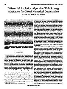
with different number of search parameters and number of objective functions. The performance metrics [1] used to evaluate the attained approximation sets with our optimizer are taken from [30]. The IH and IR2 indicators are computed (for all functions) and the CS indicator is computed for the SYMPART function. The empirical attainment surfaces are also calculated using [30]. The algorithm complexity is given at the end. This paper is organized as follows. In the next section, our new algorithm DEMOwSA is described. The third section describes the experiments and the obtained results on the test suite. The results are assessed by accompanying performance metrics. The last section concludes with final remarks and prepositions for future work. II. D IFFERENTIAL E VOLUTION FOR M ULTIOBJECTIVE O PTIMIZATION WITH S ELF A DAPTATION (DEMOW SA) As mentioned in the introduction, evolution strategies include a self-adaptive mechanism [19], encoded directly in each individual of the population to control some of the parameters in the evolutionary algorithm. An evolution strategy (ES) has a notation μ/ρ, λ-ES, where μ is parent population size, ρ is the number of parents for each new individual, and λ is child population size. An individual is denoted as a = (x, s, F (x)), where x are search parameters, s are control parameters, and F (x) is the evaluation of the individual. Although there are other notations and evolution strategies, we will only need a basic version. We use an idea of self-adaptation mechanism from evolution strategies and apply this idea to the control parameters of the candidate creation in the original DEMO algorithm [3]. We name the new constructed version of DEMO, DEMOwSA algorithm. Each individual (see Fig. 1) of DEMOwSA algorithm is extended to include self-adaptive F and CR control parameters to adjust them to the appropriate values during the evolutionary process. The F parameter is mutation control parameter and CR is the crossover control parameter. For each individual in the population, a trial vector is composed by mutation and recombination. The mutation procedure is different in the DEMOwSA algorithm in comparison to the original DEMO. For adaptation of the amplification factor of the difference vector Fi for trial individual i, from parent generation G into child generation G + 1 for the trial vector, the following formula is used: Fi,G+1 = FG i × eτ N (0,1) ,

3617 c 1-4244-1340-0/07$25.00 2007 IEEE

F1,G

CR1,G

x2,1,G

x2,2,G

x2,3,G

...

x2,D,G

F2,G

CR2,G

x3,1,G

x3,2,G

x3,3,G

...

x3,D,G

F3,G

CR3,G

...

...

xNP,1,G xNP,2,G xNP,2,G Fig. 1.

...

...

x1,D,G

...

...

...

x1,3,G

...

x1,2,G

...

x1,1,G

xNP,D,G FNP,G CRNP,G

III. R ESULTS Since the approximation set results for DEMO on CEC2007 special session test functions were not freely available on the web, nor were they ever performed for such parameter settings with same functions, we produced approximation set results for performance assessment ourselves. The DEMOwSA implementation did not exist either, so we implemented the algorithm by extending the existing DEMO code.

Encoding of the self-adapting control parameters.

A. PC Configuration where τ √ denotes learning factor and is usually proportional to τ = 1/( 2D), D being a dimension of the problem. N (0, 1) is a random number with a Gauss distribution. The FG i denotes averaging the parameter F of the current individual i and the randomly chosen individuals r1 , r2 , and r3 from the generation G: Fi,G + Fr1 ,G + Fr2 ,G + Fr3 ,G , FG i = 4 where indices r1 , r2 , and r3 are the indices of individuals also being used in the chosen DE strategy for the mutation process. The mutation process for i-th candidate vi,G+1 for generation G + 1 is defined as: vi,G+1 = xr1 ,G + Fi,G+1 × (xr2 ,G − xr3 ,G ), where xr1 ,G , xr2 ,G , and xr3 ,G are search parameter values of the uniform randomly selected parents from generation G. An analogous formula is used for the CR parameter: CRi,G+1 = CRG i × eτ N (0,1) , where τ is same as in the adaptation of F parameter and CRG i denotes averaging: CRi,G + CRr1 ,G + CRr2 ,G + CRr3 ,G . 4 Recombination process is taken from the strategy ’rand/1/bin’ used in the original DEMO [3] or the original DE [5], and the adapted CRi,G+1 is used to create a modified candidate ui,j,G+1 by binary crossover: ⎧ ⎪ ⎨vi,j,G+1 if rand(0, 1) ≤ CRi,G+1 or ui,j,G+1 = j = jrand ⎪ ⎩ xi,j,G otherwise, CRG i =

where j ∈ [1, D] denotes the j-th search parameter, rand(0, 1) ∈ [0, 1] denotes a uniformly distributed random number, and jrand denotes an uniform randomly chosen index of the search parameter, which is always exchanged. The selection principle also helps in adapting F and CR parameters, because only the individuals adapting good control and search parameter values survive. With the more appropriate values for the self-adaptive control parameters, the search process attains better objective space parameters. Therefore, the search process converges faster to better individuals which, in turn, are more likely to survive and produce offspring and, hence, propagate these better parameter values.

3618

All tests were performed on the following PC configuration. System: Linux, 2.6.17-1.2142 FC4smp. CPU: Twice 64bit Dual Core AMD Opteron(tm) Processor 280 (2390.651 MHz, 4787.74 bogomips). RAM: 8GB. Language: C++. Algorithm: DEMOwSA. B. Parameter Settings The DEMOwSA algorithm has many parameters, among which the most important are the selection algorithm and candidate creation strategy. We have chosen SPEA2 as the selection algorithm and our candidate creation strategy based on self adaptation mechanism. We have adjusted the F and CR parameters of the candidate creation process with DE. The maximal dynamic range of F parameter is F ∈ [0, 2], and for CR it is CR ∈ [0, 1]. With the applied adaptation mechanism, some control parameter constraints were used, as will be described below. The estimated cost of parameter tuning in terms of number of function evaluations is zero – only a few additional random numbers and simple calculations are conducted to express the adapted control parameters. No search is required and one control parameters adaptation is executed before each function evaluation. In the presented experiments the following parameter settings were used for our algorithm. The global lower and upper bounds for control parameter F were 0.1 ≤ F ≤ 0.9, and for control parameter CR they were 1/24 ≤ CR ≤ 0.3. Their initialization was√F = 0.5, CR = 0.3. The τ parameter was set to 1/(8 2D), which conforms to the recommendation from [19]. The population size parameter N P was set equal to approximation set size for each of the functions, i.e. 100, 150, and 800, respectively. C. Results Achieved Based on the intermediate and final resulting approximation sets of optimization process, performance assessment was induced based on CEC2007 special session performance assessment metrics. Regarding the DEMOwSA for all the test functions, an approximation set was recorded in each of the evolutionary runs after 5e+3, 5e+4, and 5e+5 function evaluations (FEs). Regarding the performance assessment suite we present: • best, median, worst, mean, and standard variance for values of the indicators IR2 and IH of all 25 runs for test functions 1–7 and 8–13 (with M = 3 and M = 5) after 5e+3, 5e+4, and 5e+5 FEs: three tables for each of

2007 IEEE Congress on Evolutionary Computation (CEC 2007)

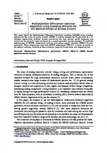
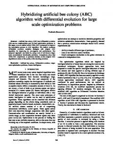
two indicators result from this requirement (see Tables I, II, III, IV, V, and VI), • best, median, worst, mean, and standard variance for values of the indicator CS of all 25 runs for test function SYMPART after 5e+3, 5e+4, and 5e+5 FEs: one table results from this requirement (see Table VII), • 0%, 50%, and 100% empirical attainment surfaces of all 25 runs for test functions 1–7 after 5e+5 FEs: a figure with seven subfigures results from this requirement (see Fig. 2), • 50% empirical attainment surfaces of all 25 runs for test functions 8-13 with M = 3, after 5e+5 FEs: one figure with six subfigures results from this requirement (see Fig. 3), • Pareto front plots after 5e+5 FEs for test functions 12 and 13 with M = 5: one figure with subfigures for each objective function combination results from this requirement (see Fig. 4), • computing time of 10,000 evaluations (T1 ) and of the same with the algorithm (T2 ) timing: one table results from this requirement (see Table VIII). From all tables, it can be observed that, from most indicator values, the algorithm is mostly successful at least to the level of attaining 0.01 close to the ideal performance metric value (which is 0). When the obtained indicator value is negative, we checked various plots and numerical data and determined that, because of the nonevenly distributed and less dense reference set than the approximation set, there are minor improvements compared to the reference set in the indicators for some of our approximations sets. From Table I, it can be seen that our algorithm performed well with respect to the given reference sets for functions OKA2, SYMPART, S ZDT1, S ZDT4, R ZDT4, and S ZDT6. The function S ZDT2 was the most difficult among these functions with regard to the R indicator. Table II shows good algorithm performance for S DTLZ2, R DTLZ2, and S DTLZ3 as also for the WFG8 and WFG9. For the function S DTLZ2, the indicator values display a small anomaly from 5e+4 FEs to 5e+5 FEs, where they get a bit worse. In this table the best solved function is WFG8 and the worst solved is WFG1, which is also true for Table III. From Tables IV, V, and VI, it can be observed that the hardest function to optimize was WFG1 with M = 3, and M = 5, whereas indicator values for the functions S ZDT6, WFG8 and WFG9 with M = 3, and the functions WFG8 and WFG9 with M = 5 are even better than the corresponding indicator values of their reference sets. IV. C ONCLUSIONS We have presented performance assessment of Differential Evolution for Multiobjective Optimization with Self Adaptation algorithm. The algorithm uses the self adaptation mechanism from evolution strategies to adapt F and CR parameters of the candidate creation in DE. Results for 25 runs on 19 test functions are presented and assessed using 4 performance metrics. Based on these metrics, the algorithm

TABLE VII T HE RESULTS FOR COVERED SETS FOR TEST FUNCTION SYMPART. FES Best Median Worst Mean Std

5e+3 1.0000e+00 1.0000e+00 1.0000e+00 1.0000e+00 0.0000e+00

5e+4 1.0000e+00 1.0000e+00 1.0000e+00 1.0000e+00 0.0000e+00

5e+5 1.0000e+00 1.0000e+00 1.0000e+00 1.0000e+00 0.0000e+00

TABLE VIII A LGORITHM C OMPLEXITY. T1 1.0600e+00 s

T2 2.7693e+01 s

(T2 − T1 )/T1 2.5130e+01

averagely attains good results on the test suite. The most problematic functions that were encountered were S ZDT4, OKA2, and WFG1. On all the remaining functions the algorithm performed better, attaining at least 0.01 proximity to the Pareto optimal set regarding the performace metrics IH and IR2 . We have already conducted a preliminary F and CR dynamics study on the algorithm, which cannot be presented here due to paper page limit, and is a good starting point for further research. Hybridizing our algorithm with local search seems to be a good idea as well. Performance assessment of DEMO with IBEA and NSGA-II has also been conducted, but the metrics and results interpretation are left for future research, although it already seems that SPEA is performing better on the test functions regarding the given quality indicators. ACKNOWLEDGMENT This work was supported in part by the Slovenian Research Agency under programme P2-0041 — Computer systems, Methodologies, and Intelligent Services. Special thanks goes to Tea Tuˇsar of Department of Intelligent Systems at the Jozef Stefan Institute, Jamova 39, SI - 1000 for providing us with the codes of the original DEMO algorithm. R EFERENCES [1] J. Knowles, L. Thiele, and E. Zitzler, “A Tutorial on the Performance Assessment of Stochastic Multiobjective Optimizers,” Computer Engineering and Networks Laboratory (TIK), ETH Zurich, Switzerland,” 214, Feb. 2006, revised version. [2] K. Deb, Multi-Objective Optimization using Evolutionary Algorithms. Chichester, UK: John Wiley & Sons, 2001, ISBN 0-471-87339-X. [3] T. Robiˇc and B. Filipiˇc, “DEMO: Differential Evolution for Multiobjective Optimization,” in Proceedings of the Third International Conference on Evolutionary Multi-Criterion Optimization – EMO 2005, ser. Lecture Notes in Computer Science, vol. 3410. Springer, 2005, pp. 520–533. [4] T. Tuˇsar and B. Filipiˇc, “Differential Evolution versus Genetic Algorithms in Multiobjective Optimization,” in Proceedings of the Fourth International Conference on Evolutionary Multi-Criterion Optimization – EMO 2007, ser. Lecture Notes in Computer Science, vol. 4403. Springer, 2007, pp. 257–271. [5] R. Storn and K. Price, “Differential Evolution – A Simple and Efficient Heuristic for Global Optimization over Continuous Spaces,” Journal of Global Optimization, vol. 11, pp. 341–359, 1997.


3619

TABLE I T HE RESULTS FOR R FES

5e+3

5e+4

5e+5

Best Median Worst Mean Std Best Median Worst Mean Std Best Median Worst Mean Std

1. OKA2 -6.2136e-04 8.4401e-04 4.0591e-03 1.0738e-03 1.1723e-03 -9.7859e-04 -3.0302e-04 9.9941e-04 -2.6206e-04 6.0745e-04 -1.0581e-03 -1.0044e-03 -1.0624e-04 -8.0507e-04 3.0496e-04

2. SYMPART 2.1494e-02 3.2792e-02 4.7681e-02 3.2867e-02 6.8335e-03 1.6145e-05 2.5157e-05 3.8961e-05 2.5823e-05 5.0663e-06 3.2744e-06 4.1441e-06 5.0803e-06 4.1873e-06 5.4693e-07

INDICATOR ON TEST FUNCTIONS

3. S ZDT1 5.3022e-02 5.8049e-02 6.7336e-02 5.9281e-02 3.9633e-03 1.4196e-04 2.4980e-04 3.0445e-04 2.4294e-04 3.7686e-05 -8.1112e-10 1.8302e-06 6.9727e-06 2.2716e-06 2.1717e-06

4. S ZDT2 1.0790e-01 1.2095e-01 1.3360e-01 1.2142e-01 6.4693e-03 3.2265e-04 6.9049e-04 4.0628e-02 1.5529e-02 1.9750e-02 0.0000e+00 3.1582e-08 4.0053e-02 1.4419e-02 1.9622e-02

1–7.

5. S ZDT4 7.5437e-02 8.4788e-02 9.3693e-02 8.5307e-02 5.0711e-03 2.4269e-02 3.0425e-02 3.5089e-02 3.0420e-02 3.0321e-03 1.7241e-03 2.7763e-03 4.5511e-03 3.0107e-03 7.3453e-04

6. R ZDT4 1.9364e-02 2.5630e-02 3.3457e-02 2.5097e-02 3.7516e-03 1.6790e-03 3.2908e-03 5.6485e-03 3.2849e-03 9.8099e-04 1.1622e-04 2.5458e-04 1.4549e-03 3.6550e-04 3.3329e-04

7. S ZDT6 1.3688e-01 1.4261e-01 1.4606e-01 1.4213e-01 2.1999e-03 2.5129e-02 2.9697e-02 4.2450e-02 3.0595e-02 4.0446e-03 -1.0216e-06 -1.0216e-06 -9.3898e-07 -1.0152e-06 2.2215e-08

TABLE II T HE RESULTS FOR R FES

5e+3

5e+4

5e+5

8. S DTLZ2 1.1818e-04 1.8319e-04 2.7839e-04 1.8734e-04 3.8855e-05 2.6126e-06 2.0169e-05 3.7881e-05 2.0590e-05 1.0259e-05 9.8209e-06 2.8298e-05 6.5781e-05 3.2122e-05 1.6826e-05



9. R DTLZ2 3.5323e-04 2.2186e-03 4.1487e-03 2.2245e-03 1.0171e-03 2.5312e-04 1.5043e-03 2.5698e-03 1.3952e-03 6.8988e-04 2.4133e-04 5.3103e-04 1.5445e-03 6.1748e-04 3.8772e-04


8–13 WHEN M = 3.

11. WFG1 5.5449e-02 5.5973e-02 5.6303e-02 5.5934e-02 2.2945e-04 5.2649e-02 5.3474e-02 5.3927e-02 5.3434e-02 3.2994e-04 2.7007e-02 3.8503e-02 4.2837e-02 3.7772e-02 3.5759e-03

12. WFG8 -1.3805e-02 -1.1809e-02 -9.7870e-03 -1.1773e-02 1.0110e-03 -2.5590e-02 -2.4526e-02 -2.2079e-02 -2.4488e-02 7.0955e-04 -2.7946e-02 -2.7509e-02 -2.7140e-02 -2.7515e-02 1.9937e-04


TABLE III T HE RESULTS FOR R FES

5e+3

5e+4

5e+5

3620






8–13 WHEN M = 5.


12. WFG8 7.3327e-03 8.9772e-03 1.1911e-02 9.3102e-03 1.2508e-03 1.4684e-03 2.9816e-03 4.8075e-03 3.0397e-03 9.8039e-04 -5.9577e-03 -3.9907e-03 -1.7535e-03 -3.9639e-03 9.9207e-04



TABLE IV T HE RESULTS FOR H YPERVOLUME INDICATOR IH ON TEST FUNCTIONS 1–7. FES

5e+3

5e+4

5e+5


1. OKA2 2.4143e-02 2.8175e-02 3.5897e-02 2.8984e-02 3.3118e-03 1.9719e-02 2.2169e-02 3.0472e-02 2.3433e-02 3.0383e-03 1.2041e-02 1.5692e-02 2.9064e-02 1.7877e-02 5.0099e-03

2. SYMPART 6.1409e-02 9.3032e-02 1.3406e-01 9.3160e-02 1.8985e-02 4.8726e-05 7.3721e-05 1.1745e-04 7.6615e-05 1.5276e-05 9.7898e-06 1.2586e-05 1.5293e-05 1.2558e-05 1.6817e-06




6. R ZDT4 5.9711e-02 7.7408e-02 9.9695e-02 7.6820e-02 9.9631e-03 5.5318e-03 1.0047e-02 1.7009e-02 1.0123e-02 2.8202e-03 3.2075e-04 7.4731e-04 4.2179e-03 1.0772e-03 9.7863e-04

7. S ZDT6 3.4675e-01 3.6269e-01 3.6999e-01 3.6117e-01 5.4189e-03 5.7133e-02 6.8166e-02 9.4732e-02 6.9641e-02 8.7574e-03 -2.3087e-04 -2.3037e-04 -2.2917e-04 -2.3035e-04 4.5290e-07

TABLE V T HE RESULTS FOR H YPERVOLUME INDICATOR IH ON TEST FUNCTIONS 8–13 WHEN M = 3. FES

5e+3

5e+4

5e+5








TABLE VI T HE RESULTS FOR H YPERVOLUME INDICATOR IH ON TEST FUNCTIONS 8–13 WHEN M = 5. FES

5e+3

5e+4

5e+5








13. WFG9 1.1185e-01 1.3650e-01 1.6541e-01 1.3861e-01 1.4118e-02 -1.0449e-01 -9.3887e-02 -8.3515e-02 -9.3784e-02 5.9951e-03 -1.2913e-01 -1.1966e-01 -1.1439e-01 -1.2020e-01 3.9269e-03

3621

1.2

2.5

’../../input/ParetoOptimalfront/OKA2’ ’../input_params/atts_OKA2-0p.out’ ’../input_params/atts_OKA2-50p.out’ ’../input_params/atts_OKA2-100p.out’

1

’../../input/ParetoOptimalfront/SYMPART’ ’../input_params/atts_SYMPART-0p.out’ ’../input_params/atts_SYMPART-50p.out’ ’../input_params/atts_SYMPART-100p.out’

2

0.8 1.5 0.6 1 0.4 0.5

0.2

0

0 -4

-3

-2

-1

0

1

2

3

4

0

0.5

(a) Test function 1 2

2

’../../input/ParetoOptimalfront/S_ZDT1’ ’../input_params/atts_S_ZDT1-0p.out’ ’../input_params/atts_S_ZDT1-50p.out’ ’../input_params/atts_S_ZDT1-100p.out’

1.9

1

1.5

2

2.5

(b) Test function 2

1.8


1.8

1.7 1.6

1.6

1.5 1.4

1.4

1.3 1.2

1.2

1.1 1

1 1

1.1

1.2

1.3

1.4

1.5

1.6

1.7

1.8

1.9

2

1

1.2

(c) Test function 3 14

11


12

1.4

1.6

1.8

2

(d) Test function 4 ’../../input/ParetoOptimalfront/R_ZDT4’ ’../input_params/atts_R_ZDT4-0p.out’ ’../input_params/atts_R_ZDT4-50p.out’ ’../input_params/atts_R_ZDT4-100p.out’

10 9

10

8 7

8

6 6

5 4

4

3 2 2 0

1 1

1.1

1.2

1.3

1.4

1.5

1.6

1.7

1.8

1.9

2

1

1.1

1.2

(e) Test function 5

1.3

1.4

1.5

1.6

1.7

1.8

1.9

2

(f) Test function 6

2


1.9 1.8 1.7 1.6 1.5 1.4 1.3 1.2 1.1 1 1.2

1.3

1.4

1.5

1.6

1.7

1.8

1.9

2

2.1

(g) Test function 7 Fig. 2.

0%, 50%, and 100% empirical attainment surfaces of all 25 runs for test functions 1–7 after 5e+5 FEs.

[6] H. A. Abbass, “The self-adaptive pareto differential evolution algorithm,” in Proceedings of the 2002 Congress on Evolutionary Computation, 2002 (CEC ’02), vol. 1, May 2002, pp. 831–836. [7] N. K. Madavan, “Multiobjective Optimization Using a Pareto Differential Evolution Approach,” in Congress on Evolutionary Computation (CEC’2002), vol. 2. Piscataway, New Jersey: IEEE Service Center, May 2002, pp. 1145–1150. [8] B. Babu and M. M. L. Jehan, “Differential Evolution for MultiObjective Optimization,” in Proceedings of the 2003 Congress on Evolutionary Computation (CEC’2003), vol. 4. Canberra, Australia: IEEE Press, December 2003, pp. 2696–2703. [9] B. V. Babu, J. H. S. Mubeen, and P. G. Chakole, “Multiobjective Op-

3622

timization Using Differential Evolution,” TechGenesis – The Journal of Information Technology, vol. 2, no. 2, pp. 4–12, 2005. [10] F. Xue, A. C. Sanderson, and R. J. Graves, “Pareto-based MultiObjective Differential Evolution,” in Proceedings of the 2003 Congress on Evolutionary Computation (CEC’2003), vol. 2. Canberra, Australia: IEEE Press, December 2003, pp. 862–869. [11] S. Kukkonen and J. Lampinen, “GDE3: The third Evolution Step of Generalized Differential Evolution,” in 2005 IEEE Congress on Evolutionary Computation (CEC’2005), vol. 1. Edinburgh, Scotland: IEEE Service Center, September 2005, pp. 443–450. [12] V. L. Huang, P. N. Suganthan, A. K. Qin, and S. Baskar, “Multiobjective Differential Evolution with External Archive and Harmonic


11 10 9 8 7 6 5 4 3 2 1

0

9000 8000 7000 6000 5000 4000 3000 2000 1000 0

2

4

6

8

10

12 11 10

9

8

7

5

6

4

2

3

0 1000 2000 3000 4000 5000 6000 1000 0 7000 400030002000 8000 900090008000700060005000

1

(a) Test function 8 (S DTLZ2 with M = 3).

(b) Test function 9 (R DTLZ2 with M = 3).

7000 6000 5000 4000 3000 2000 1000 0

11 10 9 8 7 6 5 4 3 2 1 0

0 1000 2000 3000 4000 5000 3000 2000 1000 6000 70007000 6000 5000 4000

0

2

4

0

(c) Test function 10 (S DTLZ3 with M = 3).

2

0 4

6

8

10

12 12

Fig. 3.

[14]

[15]

[16]

10

12 11 10 9

7

8

5

6

3

4

2

1

0

12 10 8 6 4 2 0

10

8

6

4

2

0

(e) Test function 12 (WFG8 with M = 3).

[13]

8

(d) Test function 11 (WFG1 with M = 3).

12 10 8 6 4 2 0

0

6

2

4

6

8

10

12 12

10

8

6

4

2

0

(f) Test function 13 (WFG9 with M = 3).

50% empirical attainment surfaces of all 25 runs for test functions 8–13 with M = 3 after 5e+5 FEs.

Distance-Based Diversity Measure,” Nanyang Technological University, Singapore, Tech. Rep. TR-07-01, 2006. L. V. Santana-Quintero and C. A. Coello Coello, “An Algorithm Based on Differential Evolution for Multi-Objective Problems,” International Journal of Computational Intelligence Research, vol. 1, no. 2, pp. 151– 169, 2005. A. W. Iorio and X. Li, “Incorporating Directional Information within a Differential Evolution Algorithm for Multi-objective Optimization,” in 2006 Genetic and Evolutionary Computation Conference (GECCO’2006), M. K. et al., Ed., vol. 1. Seattle, Washington, USA: ACM Press. ISBN 1-59593-186-4, July 2006, pp. 691–697. A. G. Hernández-D´ıaz, L. V. Santana-Quintero, C. C. Coello, R. Caballero, and J. Molina, “A new proposal for multi-objective optimization using differential evolution and rough sets theory,” in Proceedings of the 8th annual conference on Genetic and evolutionary computation — GECCO 2006, vol. 1, 2006, pp. 675–682. K. Deb, S. Agrawal, A. Pratab, and T. Meyarivan, “A Fast Elitist NonDominated Sorting Genetic Algorithm for Multi-Objective Optimization: NSGA-II,” in Proceedings of the Parallel Problem Solving from Nature VI Conference, M. Schoenauer, K. Deb, G. Rudolph, X. Yao, E. Lutton, J. J. Merelo, and H.-P. Schwefel, Eds. Paris, France: Springer. Lecture Notes in Computer Science No. 1917, 2000, pp.

849–858. [17] E. Zitzler, M. Laumanns, and L. Thiele, “SPEA2: Improving the Strength Pareto Evolutionary Algorithm for Multiobjective Optimization,” in Evolutionary Methods for Design Optimization and Control with Applications to Industrial Problems, K. C. Giannakoglou, D. T. Tsahalis, J. Périaux, K. D. Papailiou, and T. Fogarty, Eds. Athens, Greece: International Center for Numerical Methods in Engineering (Cmine), 2001, pp. 95–100. [18] E. Zitzler and S. Ku¨ nzli, “Indicator-Based Selection in Multiobjective Search,” in Parallel Problem Solving from Nature (PPSN VIII), X. Yao et al., Eds. Berlin, Germany: Springer-Verlag, 2004, pp. 832–842. [19] H.-G. Beyer and H.-P. Schwefel, “Evolution strategies — A comprehensive introduction,” Natural Computing, vol. 1, pp. 3–52, 2002. [20] T. Bäck, Evolutionary Algorithms in Theory and Practice: Evolution Strategies, Evolutionary Programming, Genetic Algorithms. New York: Oxford University Press, 1996. [21] H.-P. Schwefel, Evolution and Optimum Seeking, ser. Sixth-Generation Computer Technology. New York: Wiley Interscience, 1995. ˇ [22] J. Brest, S. Greiner, B. Boˇsković, M. Mernik, and V. Zumer, “SelfAdapting Control Parameters in Differential Evolution: A Comparative Study on Numerical Benchmark Problems,” IEEE Transactions on Evolutionary Computation, vol. 10, no. 6, pp. 646–657, 2006, DOI:


3623

f_1 1.0 − 2.0

f_2 1.0 − 2.0

f_3 1.0 − 2.0

f_4 1.0 − 2.0

f_5 1.0 − 2.0 Fig. 4. Pareto front plots of the median approximation set with respect to the R indicator after 5e+5 FEs for test functions 12 and 13 with M = 5. Upper diagonal plots are for WFG8 (M=5) and lower diagonal plots are for WFG9 (M=5). The axes of any plot can be obtained by looking at the corresponding diagonal boxes and their ranges. For WFG8, the label in a column denotes the abscissa and the label in a row denotes the ordinate, and contrary for WFG9.

10.1109/TEVC.2006.872133. ˇ [23] J. Brest, V. Zumer, and M. S. Mauˇcec, “Self-adaptive Differential Evolution Algorithm in Constrained Real-Parameter Optimization,” in The 2006 IEEE Congress on Evolutionary Computation CEC2006. IEEE Press, 2006, pp. 919–926. [24] V. L. Huang, A. K. Qin, K. Deb, E. Zitzler, P. N. Suganthan, J. J. Liang, M. Preuss, and S. Huband, “Problem Definitions for Performance Assessment & Competition on Multi-objective Optimization Algorithms,” Nanyang Technological University et. al., Singapore, Tech. Rep. TR07-01, 2007. [25] T. Okabe, Y. Jin, M. Olhofer, and B. Sendhoff, “On Test Functions for Evolutionary Multi-objective Optimization,” in PPSN, 2004, pp. 792–802. [26] G. Rudolph, B. Naujoks, and M. Preuss, “Capabilities of EMOA to Detect and Preserve Equivalent Pareto Subsets,” in Evolutionary MultiCriterion Optimization (EMO 2007), vol. 4403. Springer, 2007, pp. 36–50.

3624

[27] E. Zitzler, K. Deb, and L. Thiele, “Comparison of Multiobjective Evolutionary Algorithms: Empirical Results,” Evolutionary Computation, vol. 8, no. 2, pp. 173–195, Summer 2000. [28] K. Deb, L. Thiele, M. Laumanns, and E. Zitzler, “Scalable MultiObjective Optimization Test Problems,” in Congress on Evolutionary Computation (CEC’2002), vol. 1. Piscataway, New Jersey: IEEE Service Center, May 2002, pp. 825–830. [29] S. Huband, P. Hingston, L. Barone, and L. While, “A Review of Multiobjective Test Problems and a Scalable Test Problem Toolkit,” IEEE Transactions on Evolutionary Computation, vol. 10, no. 5, pp. 477–506, October 2006. [30] S. Bleuler, M. Laumanns, L. Thiele, and E. Zitzler, “PISA — A Platform and Programming Language Independent Interface for Search Algorithms,” in Evolutionary Multi-Criterion Optimization (EMO 2003), ser. Lecture Notes in Computer Science, C. M. Fonseca, P. J. Fleming, E. Zitzler, K. Deb, and L. Thiele, Eds. Berlin: Springer, 2003, pp. 494–508.
