IEEE GEOSCIENCE AND REMOTE SENSING LETTERS, VOL. XX, NO. X, MARCH 2017. 1. R. Diffusion-Based Inpainting for Coding. Remote-Sensing Data.
IEEE GEOSCIENCE AND REMOTE SENSING LETTERS, VOL. XX, NO. X, MARCH 2017
1
Postprint of: Amrani, Naoufal et al. “Diffusion-based inpainting for coding remotesensing data” in IEEE Geoscience and Remote Sensing Letters, March 2017.
Diffusion-Based Inpainting for Coding Remote-Sensing Data Naoufal Amrani† , Joan Serra-Sagristà† , Pascal Peter‡ and Joachim Weickert‡ of Information and Communications Engineering, Universitat Autònoma de Barcelona ‡ Mathematical Image Analysis Group, Saarland University
† Department
Abstract—Inpainting techniques based on partial differential equations (PDEs) such as diffusion processes are gaining growing importance as a novel family of image compression methods. Nevertheless, the application of inpainting in the field of hyperspectral imagery has been mainly focused on filling in missing information or dead pixels due to sensor failures. In this paper we propose a novel PDE-based inpainting algorithm to compress hyperspectral images. The method inpaints separately the known data in the spatial and in the spectral dimensions. Then it applies a prediction model to the final inpainting solution to obtain a representation much closer to the original image. Experimental results over a set of hyperspectral images indicate that the proposed algorithm can perform better than a recent proposed extension to prediction-based standard CCSDS-123.0 at low bitrate, better than JPEG 2000 Part 2 with the DWT 9/7 as a spectral transform at all bit-rates, and competitive to JPEG 2000 with principal component analysis (PCA), the optimal spectral decorrelation transform for Gaussian sources.
I. I NTRODUCTION EMOTE sensing data provides a large amount of spatial, spectral and temporal information about the earth surface. It must meet the needs of a wide range of important applications requiring fine and frequent coverage of large areas. The increasing number of high resolution sensors present a tough challenge for current storage and transmission systems. For instance, the NASA instrument Airborne Visible Infrared Imaging Spectrometer (AVIRIS) [1] delivers images of the upwelling spectral radiance in 224 contiguous spectral channels with wavelengths from 400 to 2500 nanometers (nm). Hence, the need for efficient coding techniques for remote-sensing data becomes more and more imperative to improve the capabilities of storage and transmission. Most of these coding techniques for remote-sensing data are dominated by transform-based concepts that exploit the redundancy in the spatial and in the spectral dimensions. Typically, a compression technique applies a 1D spectral transform followed by a 2D spatial transform usually based on wavelets. Nevertheless, the predictive methods gain more importance for lossless and near-lossless coding. For instance, the M-CALIC algorithm [2], the standard CCSDS-123.0 [3] and a recent proposed extension of CCSDS-123.0 [4] can outperform the transform-based methods for high-quality and lossless coding. Other recently proposed works combine transform- and predictive-based methods using regression
R
This work was supported in part by the Spanish Ministry of Economy and Competitiveness (MINECO), by the European Regional Development Fund (FEDER) and by the European Union (EU) under Grant TIN2015-71126-R, and by the Catalan Government under Grant 2014SGR-691.
analysis to tackle the dependencies that still remain among the data in the transform domain. These techniques provide promising results for lossless and progressive lossy-to-lossless coding [5], [6], [7], [8]. Besides the aforementioned techniques, a new family of compression algorithms based on partial differential equations (PDEs) has emerged in the last years for coding 2D images [9], with extensions to color [10] and 3D medical images [11]. The idea relies on storing only a small selected subset of the image pixels, and reconstructing the remainder of the image by inpainting with a partial differential equation (PDE) such as a diffusion process. However, in the field of hyperspectral imagery, the use of PDEs and other interpolation-based methods focuses on denoising or filling in dead pixels and missing information due to sensor failure or malfunction [12]. To the best of our knowledge, no approach to date has considered PDE-based inpainting for compressing hyperspectral images. Several factors make the application of PDEs and interpolation-based methods for coding remotesensing data a difficult and complex task, entailing the need for sophisticated techniques to provide competitive results. Among these factors are the structural surfaces, the highdimensionality of the data and the degradation mechanism due to the sensor characteristics. In this respect, common PDE approaches that lead to a smooth recovery may not be appropriate for hyperspectral images. On the other hand, successful PDE approaches addressed for denoising or filling missing information in hyperspectral images do not account for compression constraints related to the efficient selection and storage of the known data [13]. In this paper, we focus on simpler inpainting operators like homogeneous and biharmonic ones, while adopting the transform-based idea of exploiting separately the spatial and spectral redundancy. Moreover, a prediction step is performed to reduce the reconstruction error. Building upon that, this paper introduces a novel 2D+1D+h(·) diffusion-based scheme for coding hyperspectral images. The idea is based on applying three basic steps. First, 2D homogeneous diffusion inpainting is applied in the spatial dimensions, then the difference between the original image and the 2D inpainting solution is computed. Second, a 1D biharmonic inpaining is applied to this difference in the spectral dimension. Finally, the 2D+1D inpainting solution is used by a prediction model h(·) to give a representation much closer to the original image. Our paper is organized as follows. Section II reviews the PDE-based interpolation and formulates the discrete problem.
2
IEEE GEOSCIENCE AND REMOTE SENSING LETTERS, VOL. XX, NO. X, MARCH 2017
Section III introduces our inpainting scheme to encode hyperspectral images. Section IV provides the experimental results and Section V concludes the paper. II. PDE-B ASED I NPAINTING AND C OMPRESSION In this section we describe the PDE-based inpainting problem and the discrete formulation. Afterwards we explain the mask selection and the optimization of gray values.
We can proceed similarly for a 1D inpainting process in the spectral dimension. Using a binary mask ci ∈ Rz for a spectral pixel xi∗ = (fi,j )j∈ Z ∈ Rz , where Z = {1, · · · , z}, the linear system to solve is (Ci − (Iz×z − Ci ) L) v i∗ = Ci xi∗ .
(5)
Here v i∗ ∈ R z is the inpainting solution, and Ci ∈ {0, 1} z×z z is a diagonal matrix having the mask vector ci ∈ {0, 1} as the main diagonal entries.
A. PDE compression model Let f : Ω → R denote an image that maps a domain Ω to the corresponding values. Let ΩK ⊂ Ω be a subset of the image domain where the original image f is known. Diffusion-based inpainting aims at computing a reconstruction image u : Ω → R that reproduces the missing parts of f on the inpainting domain Ω \ ΩK based on smoothness assumptions. To this end, one solves the PDE (1 − c(x))Lu − c(x)(u − f ) = 0,
(1)
where u is the inpainting solution, L is a differential operator, and the characteristic function c(x) specifies whether a point is known or not: c(x) =
1 if x ∈ ΩK 0 if x ∈ Ω \ ΩK .
(2)
This guarantees that on ΩK , f is reproduced perfectly, i.e. the known data stays fixed. Together with reflecting boundary conditions on the outer image boundaries ∂Ω, the inpainting equation (1) leads to a propagation of the known data into the missing areas according to the smoothness constraints imposed by the differential operator L. Typical choices include the Laplacian L = ∆ and the biharmonic operator L = −∆2 . In contrast to other contexts such as denoising or filling in corrupted areas, the basic idea of PDE-based methods in the compression context is to reduce the image data to a set of sparse points that can be encoded efficiently. The decoding consists then of interpolating these scattered points in order to achieve an approximation of the original image. B. Discrete formulation To provide the necessary notation for a discrete hyperspectral image, a discrete formulation of (Eq.1) is needed. Let f = [f ∗1 , · · · , f ∗z ] ∈ Rm×z be a hyperspectral image with z spectral bands and m = x × y spatial samples. Each band f ∗j = (fi,j )i∈I ∈ R m is reshaped to a vector, where I = {1, · · · , m} denotes the pixel indices. For a 2D inpainting process in the spatial dimensions using m a binary mask cj ∈ {0, 1 } for a band f ∗j ∈ Rm , the discrete equation that we have to solve is m
(Im×m − Cj ) Lu∗j − Cj u∗j − f ∗j = 0 ∈ {0} ,
(3)
where u∗j ∈ Rm denotes the solution vector, Cj ∈ m×m {0, 1} is a diagonal matrix having the mask vector cj ∈ {0, 1}m as the main diagonal entries, Im×m is the identity matrix and L ∈ Rm×m is a square matrix describing the discrete differential operator. (Eq.3) can be formulated as a linear system with a unique solution: (Cj − (Im×m − Cj ) L) u∗j = Cj f ∗j .
(4)
C. Mask selection In addition to the differential operator, the selection of the mask that indicates the location of the known data plays a key role in reconstructing the image. Selecting this mask by using heuristics based on grid subdivision results in an efficient storage, but usually not in an efficient reconstruction. In this paper, we apply two optimization approaches [14]. The first one is called probabilistic sparsification. It starts by considering all the data points (|J |) and iteratively removes the least significant pixels until only a desired density 0 < d < 1 of the known pixels |K | = d·|J | remains. Specifically, in each iteration the following steps are applied: 1. Initialize |K | = |J |. 2. Remove a random fraction p · |J | of candidates pixels, and apply inpainting. 3. Compute the reconstruction error for these p · |J | pixels. 4. Remove a small fraction q · p · |J | of the candidate pixels with the smallest error. 5. Update K = K \ {removed pixels}. 6. Repeat the steps (2) to (5) while |K | > d · |J |. The second approach is called non-local pixel exchange. It is a post-optimization step that allows to improve the results of any previously selected mask. In each iteration, a set T of m non-mask pixel is randomly selected from J \ K as candidates and the local error ei is computed for all i ∈ T . Then, n < |T | pixel indices i are randomly selected from K , and exchanged with n pixels from T with the largest error ei . If the inpainting solution is worse than before, we revert the switch. Otherwise we proceed with the new mask. D. Gray value optimization Usually in inpainting, the original gray values of the input image f are used to propagate the information in the missing positions. However, allowing arbitrary gray values may lead, in global, to a better reconstruction, even though some error is locally introduced in the known data. The gray value optimization approach [14] uses least square approximation to find the optimal gray values g that minimize the mean squared error for a given mask c. If we denote by u = r(c, f ) the inpainting solution for a given mask c, then the minimization becomes argmin kf − r(c, g)k22 .
(6)
g∈K
III. P ROPOSED DIFFUSION SCHEME The main idea of our inpainting scheme is (i) to exploit separately the spectral and the spatial redundancy, and (ii) to
3
apply a prediction function to the inpainting solution in order to minimize the reconstruction error. The first point is motivated by the fact that the relationships among the data coefficients are significantly different in the spatial dimensions than in the spectral dimension. Usually, the spectral correlation is much higher than the spatial one, and the spectral variation is much slower. This results in a high correlation not only between neighbor bands, but also between bands widely separated. As a result, separately exploiting the redundancy in each dimension has proven to be the most appropriate model of hyperspectral data for many families of compression techniques. For instance, the transform-based coders achieve better performance by applying a spectral transform followed by a spatial one [15]. The second point is motivated by the fact that the inpainting solution may be highly correlated with the reconstruction error. Hence, a prediction model that exploits this correlation will provide an estimation much closer to the original image. Following the previous intuitions, our scheme is formed by three basic steps. First, a 2D inpainting is applied in the spatial dimensions to each band. Then the difference between the original image and the inpainting solution is computed. Second, a 1D spectral inpainting is applied to this difference, which usually still exhibits large spectral correlation, since only a 2D diffusion reconstruction has been removed from the original image. Finally, a prediction model is applied to the sum of the inpainting solutions 2D+1D to minimize the reconstruction error. In what follows we explain these three steps with more details.
Finally, the difference between the original image and the 2D inpainting solution is computed to yield r ∗j =f ∗j −u∗j ∈R m . This difference, the so-called residual, represents the information that was not accurately reconstructed by the spatial diffusion inpainting. Since the residual is still highly correlated in the spectral dimension, we aim at removing this redundancy with 1D diffusion inpainting in the following. C. 1D biharmonic diffusion Note that from the original image we removed a 2D inpainting solution based on exploiting the spatial redundancy using a fixed mask. Thus, the residual r2d = [r 1 ∗ , · · · , r m∗ ]> ∈ Rm×z (seen as a set of m spectral vectors r i ∗ ∈ Rz ) usually still exhibits a large correlation along the spectral dimension. To illustrate that, Fig. 1 depicts the correlation matrices of an original image and the difference image after removing a 2D inpainting solution obtained from using 5% of spatial pixels. Note that the correlation among spectral bands is largely maintained, while the variance is significantly reduced. The 1D inpainting aims at reconstructing an approximation of 1 224 1
56
112
1 224 1
56
56
112
112
56
112
1
0.5
A. Differential operator In this paper we deal with two operators: the homogeneous (a) Original (σ 2 =2.35×10⁵ ) (b) Residual (σ 2 =1.17×10⁴ ) diffusion operator that uses the Laplacian Lu := ∂xx u + ∂yy u to be applied in the spatial dimensions, and the biharmonic Fig. 1: Correlation matrices for AVIRIS Yellowstone sc 00 operator Lu := −∂zzzz u to be applied in the spectral Radiance (224 components). dimension. These choices are based on the results of extensive r2d using a small number of points. Again, for an efficient experiments over a set of hyperspectral images. storage we select a fixed mask c1d ∈ Rz for all the spectral vectors r i∗ ∈ R z , i.e., we seek for a reconstruction of B. 2D homogeneous diffusion r2d from a small number of bands. The mask selection is Let f = [f ∗1 , · · · , f ∗z ] ∈ Rm×z be a hyperspectral image. performed through nonlocal pixel exchange applied in the From each spectral band f ∗j ∈ Rm only a small number spectral dimension, having as initial mask the one obtained of pixels is selected using probabilistic sparsification. For an by applying probabilistic sparsification. efficient storage, the same fixed mask c2d is selected for all To provide the best inpainting solution using the selected the spectral bands f ∗j . To achieve that, the random selection mask, the gray value optimization is applied to find the gray in Step 2 chooses the same positions for all the bands. Then values that minimize the error between r2d and the biharmonic Step 3 computes the mean square error of each position along inpainting solution v. Let g ∈ Rm×z be an image containing all the spectral bands. Finally, Step 4 removes the pixels with the optimized values in the mask positions and the unknown the smallest error. data in the complement positions. Then (Eq.5) is solved using Once the mask is selected, the homogeneous inpainting is g instead of f . The solution can be expressed in the following applied in the spatial dimensions using (Eq.4) for each band matrix form: f ∗j . The solution equation can be expressed in the following C 1d − (Iz×z − C 1d ) A2 v i∗ = C 1d g i∗ , (8) matrix form: 224
(C2d − (Im×m − C2d ) A) u∗j = C2d f ∗j ,
(7)
where A ∈ Rm×m is a symmetric square matrix describing the discrete Laplacian operator with reflecting boundary conm×m ditions, C2d ∈ {0, 1} is a diagonal matrix having the m mask vector c2d ∈ {0, 1} as the main diagonal entries, and u∗j ∈ R m is the inpainting solution.
224
0
where v i∗ ∈ Rz is the biharmonic inpainting solution of ri∗ and C1d ∈ {0, 1}z×z is a diagonal matrix having the mask z vector c 1d ∈ {0, 1} as the main diagonal entries. With this step, the global 2D + 1D inpainting solution of f = u + r2d becomes w = u + v = [w ∗1 , · · · , w∗z ] ∈ R m×z .
(9)
4
IEEE GEOSCIENCE AND REMOTE SENSING LETTERS, VOL. XX, NO. X, MARCH 2017
D. Prediction model The quality of the inpainting solution can be described by the reconstruction error e = f − w. The smaller the error, the better the quality. However, some statistical relationships may exist between the inpainting solution and the reconstruction error, i.e., part of this error can be described by the reconstructed image. Here, we propose a prediction model that exploits these statistical relationships. The idea is to predict each original band f j from the bands of the
also called known data. Given a density d, the known data is selected through the previously described probabilistic sparsification or non-local pixel exchange approaches [14]. However, following our 2D+1D scheme, the selection of the known data is performed twice. First, a fraction d2 is spatially selected from the original image. Then another fraction d1 is spectrally selected from the residual r2d , with d = d1 + d2 . Distributing this data equally may not be the most appropriate choice. Beyond the pixel magnitudes or
∗
2D+1D inpainting solution through a prediction function hj (·) in order to minimize the reconstruction error: f ∗j = hj (w) + e0∗j .
(10)
Any suitable prediction function hj (·) could be applied to remove the aforementioned dependencies. In our experiments, we used a linear regression model that takes as input entries for predicting a band f some adjacent bands to that of index ∗j
j from the 2D and 1D inpainting solutions. Specifically, the proposed model is as follows: hj (w) =fb ∗j =βj,0 +βj,1 u∗j−2 + · · · +βj,5 u∗i+2 + αj,1 v ∗j−2 + · · · + αj,5 v ∗j+2 .
the variance, which is usually much lower for the residual r2d than for the original image, the main issue consists of analyzing in which dimension it is more favorable to invest more pixels. To this end, Fig. 3 depicts the coding performance of our inpainting scheme (2D+1D+h(·)) applied to a hyperspectral image using different distributions. As can be seen, selecting more pixels from the residual r2d for the 1D spectral inpainting is beneficial for compression. For a given global density d, we used a distribution of d2 = 0.25·d for 2D inpainting and d1 = 0.75 · d for 1D inpainting. This choice has experimentally been shown to provide a good trade-off between coding cost and quality gain.
(11) 50
The parameters α = (αj,· )j∈Z and β = (βj,· )j∈Z are found by using the least squares method that minimizes the squared distances between f ∗j and fb ∗j . The final 2D+1D+h(·) representation becomes
48
46
(12)
SNR (dB)
44
h (w) = [h1 (w) , · · · , hz (w)] ∈ Rm×z .
4 2
To illustrate the prediction step, Fig. 2a depicts a cross40 2D 10% 1D correlation matrix of w and e. It contains the pairwise 90% 38 2D 25% 1D correlations (in terms of the squared correlation coefficient 75% r 2 ) of each pair (w ∗j , e∗j0 ) formed by one component from 36 2D 50% 0.4 0.5 0.6 0.7 0.8 0.9 1D1.0 1.1 Bitrate the 2D+1D inpainting solution w and one component from (bpppc) the error image e. Furthermore, Fig. 2b shows the crosscorrelation matrix of h(w) and e0 after applying the prediction Fig. 3: Different distributions of the known data for AVIRIS model (Eq.11). The reconstruction has been achieved by using Yellowstone sc 00 Radiance (224 components). 10% of pixels from a typical hyperspectral image with 224 spectral bands. As can be seen, the proposed regression model efficiently exploits the correlation and significantly reduces IV. E XPERIMENTAL RESULTS the reconstruction error. In this section we evaluate our diffusion-based coder for a set of hyperspectral images from AVIRIS, CASI and AIRS h( W sensors. For comparison purposes, we provide results for a rew) cent extension of prediction-based standard CCSDS-123.0 [4] and for the JPEG 2000 Part 2 standard applying different spectral transforms, including the PCA transform and the spectral DWT 9/7 (8 levels) before the 2D spatial DWT 9/7 e with 5 levels. The Kakadu software implementation of JPEG 2000 has been used. For all the experiments, we used the parameters p=q=0.1 for probabilistic sparsification. For nonlocal pixel exchange, we used the parameters m = 10, n = 1, (a) Correlation: P 2e vs. w. (b) Correlation: e0 vs. h(w). and 1000 iterations as a stopping criterion. The known data M SE = 1 1 P 02 i e = 653.7 1 224 1
56
112
1
56 224
1
112
1
e0 = f−h(w)
56
56
112
112
0.5
224
0
224
n
i
M SE =
n
i ei
= 49.9
Fig. 2: Cross-correlation matrices for AVIRIS Yellowstone sc 10 Radiance (224 components).
E. Known data distribution As said, the idea of PDE-based image compression relies on storing a small fraction (a density d) of image pixels,
has been decorrelated losslessly by the RWA transform [5], and compressed by the PAQ software [16] . Figure 4 provides the rate-distortion performance for the transform-based methods applied to the Hawaii uncalibrated image. Table I reports the results of our algorithm as compared to [4]. The rate-distortion performance is assessed through the relation between the target bitrate, measured in bits per pixel per component (bpppc), and the reconstruction
5
quality, measured as the signal-to-noise ratio (SNR), comP P 2 2 ˆ2 puted as 10 log10 i,j,k (fi,j,k − fi,j,k ) . i,j,k f i,j,k / 46 44 42 40
SNR (dB)
38 36
34
Inpainting 2D+1D+h( · ) JPEG2000 part II (DWT 97)
32 30 28 0.0 1.4
0.2
0.4
0.6
0.8
1.0
1.2
The scheme propagates the known information separately in the spatial and in the spectral dimensions, then reduces the reconstruction error by applying a prediction model to the final inpainting solution. The prediction step shows that the quality of the inpainting solution relies not only on the extent of the reconstruction error, but also on the capability of this solution to estimate the original image using a suitable prediction model. The proposed 2D+1D+h(·) scheme provides competitive results to the most prominent state-ofthe-art standard JPEG 2000 Part 2 and to an extension of the prevailing standard CCSDS-123.0.
Bitrate (bpp)
Fig. 4: Rate-Distortion performance for Hawaii uncalibrated (512 rows, 614 columns and 224 bands).
TABLE I: Comparison between our 2D+1D+h(·) and the recently proposed extension to CCSDS-123.0 [4] Image
2D+1D+h(·)
Ext. CCSDS-123.0 [4]
rate (bpppc)
SNR (dB)
rate (bpppc)
SNR (dB)
YST 00 uncal 512 rows 680 columns 224 bands
0.36 0.48 1.07 2.00
34.38 37.57 48.04 53.66
0.35 0.53 1.01 2.00
32.34 36.20 46.42 55.96
AIRS-GRAN9 135 rows 90 columns 1501 bands
0.28 0.50 1.00 2.02
56.06 57.03 58.10 61.58
0.28 0.50 1.00 2.02
36.38 46.82 53.91 63.21
CASI-T0477F 1225 rows 406 columns 72 bands
0.36 0.53 1.03 2.03
25.73 28.57 38.62 47.14
0.37 0.52 1.01 2.03
19.90 23.79 40.53 50.61
In general, our inpainting-based approach performs better than JPEG 2000 Part 2 with the DWT 9/7 in the spectral dimension and it is competitive to PCA spectral transform, which is the optimal decorrelation transform for Gaussian sources. When compared to a prediction-based approach, our inpainting scheme is superior to [4] at high compression ratios, usually even up to a bit-rate of 1 bpppc, while at moderate to low compression ratios, our approach lags behind, a prevalent behaviour when comparing transform-based and prediction-based approaches [17], [18]. With regard to the impact of the prediction model h(·), Fig. 5 provides the rate-distortion performance for our inpainting scheme with and without the prediction step. As can be seen, the prediction model significantly improves the performance, in some cases by more than 10 dB. 60 55 50
SNR (dB)
45 40 35
Yellowstone: 2D+1D Yellowstone: 2D+1D+h( ·)
30 25 20 0.0
Maine: 2D+1D 0.5
Maine: 2D+1D+h( ·) 1.0 1.5 2.0 Bitrate Hawaii: 2D+1D (bpppc)
2.5
Fig. 5: Prediction impact for uncalibrated AVIRIS images
V. C ONCLUSION Diffusion-based inpainting has shown to be useful for image compression. In this paper we proposed a diffusionbased inpainting algorithm for coding hyperspectral images.
R EFERENCES [1] Jet Propulsion Laboratory, NASA. [Online]. Available: http://aviris.jpl.nasa.gov/html/aviris.overview.html [2] E. Magli, G. Olmo, and E. Quacchio, “Optimized onboard lossless and near-lossless compression of hyperspectral data using CALIC,” IEEE Geoscience and Remote Sensing Letters, vol. 1, no. 1, pp. 21–25, Jan. 2004. [3] Consultative Committee for Space Data Systems (CCSDS), Lossless Multispectral & Hyperspectral Image Compression CCSDS 123.0-B-1, ser. Blue Book. CCSDS, May 2012. [4] M. Conoscenti, R. Coppola, and E. Magli, “Constant SNR, rate control, and entropy coding for predictive lossy hyperspectral image compression,” IEEE Transactions on Geoscience and Remote Sensing, vol. 54, no. 12, pp. 7431–7441, Dec 2016. [5] N. Amrani, J. Serra-Sagrista, V. Laparra, M. Marcellin, and J. Malo, “Regression wavelet analysis for lossless coding of remote-sensing data,” IEEE Transactions on Geoscience and Remote Sensing, vol. 54, in press, 2016. [6] N. Amrani, J. Serra-Sagrista, M. Hernandez-Cabronero, and M. Marcellin, “Regression wavelet analysis for progressive-lossy-to-lossless coding of remote-sensing data,” in Data Compression Conference, March 2016. [7] N. Amrani, J. Serra-Sagrista, and M. Marcellin, “Unbiasedness of regression wavelet analysis for progressive lossy-to-lossless coding,” in Picture Coding Symposium, December 2016. [8] N. Amrani, M. Serra-Sagrista, and M. Marcellin, “Low complexity prediction model for coding remote-sensing data with regression wavelet analysis,” in Data Compression Conference, April 2017. [9] I. Galic´, J. Weickert, M. Welk, A. Bruhn, A. Belyaev, and H.-P. Seidel, “Towards PDE-based image compression,” in Variational, Geometric, and Level Set Methods in Computer Vision. Springer, 2005, pp. 37–48. [10] P. Peter, L. Kaufhold, and J. Weickert, “Turning diffusion-based image colorization into efficient color compression,” IEEE Transactions on Image Processing, vol. 26, no. 2, pp. 860–869, Feb. 2017. [11] C. Schmaltz, P. Peter, M. Mainberger, F. Ebel, J. Weickert, and A. Bruhn, “Understanding, optimising, and extending data compression with anisotropic diffusion,” International Journal of Computer Vision, vol. 108, no. 3, pp. 222–240, 2014. [12] H. Shen, X. Li, Q. Cheng, C. Zeng, G. Yang, H. Li, and L. Zhang, “Missing information reconstruction of remote sensing data: A technical review,” IEEE Geoscience and Remote Sensing Magazine, vol. 3, no. 3, pp. 61–85, 2015. [13] J. Martin-Herrero, “Anisotropic diffusion in the hypercube,” IEEE Transactions on Geoscience and Remote Sensing, vol. 45, no. 5, pp. 1386–1398, 2007. [14] M. Mainberger, S. Hoffmann, J. Weickert, C. H. Tang, D. Johannsen, F. Neumann, and B. Doerr, “Optimising spatial and tonal data for homogeneous diffusion inpainting,” in International Conference on Scale Space and Variational Methods in Computer Vision. Springer, 2011, pp. 26–37. [15] B. Penna, T. Tillo, E. Magli, and G. Olmo, “Transform coding techniques for lossy hyperspectral data compression,” IEEE Transactions on Geoscience and Remote Sensing, vol. 45, no. 5, pp. 1408–1421, May 2007. [16] “The PAQ Data Compression Programs.” [Online]. Available: http://www.mattmahoney.net/dc/paq.html [17] E. Magli, “Multiband lossless compression of hyperspectral images,” IEEE Transactions on Geoscience and Remote Sensing, vol. 47, no. 4, pp. 1168–1178, Apr 2009. [18] D. Valsesia and E. Magli, “A novel rate control algorithm for onboard predictive coding of multispectral and hyperspectral images,” IEEE Transactions on Geoscience and Remote Sensing, vol. 52, no. 10, pp. 6341–6355, Oct 2014.


![Inpainting [PDF]](https://m.moam.info/img/260x300/inpainting-pdf_648c3831098a9eec498b4579.jpg)