Diffusion dynamics on multiplex networks

Diffusion dynamics on multiplex networks S. Gómez,1 A. D´ıaz-Guilera,2, 3 J. Gómez-Gardeñes,3, 4 C.J. Pérez-Vicente,2 Y. Moreno,3, 5 and A. Arenas1, 3 1

arXiv:1207.2788v2 [physics.soc-ph] 3 Dec 2012

Departament d’Enginyeria Informàtica i Matemàtiques, Universitat Rovira i Virgili, Tarragona, Spain 2 Departament de F´ısica Fonamental, Universitat de Barcelona, Barcelona, Spain 3 Institute for Biocomputation and Physics of Complex Systems (BIFI), Universidad de Zaragoza, 50018 Zaragoza, Spain 4 Departamento de F´ısica de la Materia Condensada, Universidad de Zaragoza, 50009 Zaragoza, Spain 5 Departamento de F´ısica Teórica, Universidad de Zaragoza, 50009 Zaragoza, Spain We study the time scales associated to diffusion processes that take place on multiplex networks, i.e. on a set of networks linked through interconnected layers. To this end, we propose the construction of a supra-Laplacian matrix, which consists of a dimensional lifting of the Laplacian matrix of each layer of the multiplex network. We use perturbative analysis to reveal analytically the structure of eigenvectors and eigenvalues of the complete network in terms of the spectral properties of the individual layers. The spectrum of the supra-Laplacian allows us to understand the physics of diffusion-like processes on top of multiplex networks. PACS numbers: 89.75.Hc,89.20.-a,89.75.Kd

Modern theory of complex networks is facing new challenges that arise from the necessity of understanding properly the dynamical evolution of real systems. One of such open problems concerns the topological and dynamical characterization of systems made up by two or more interconnected networks. The standard approach in network modeling assumes that every edge (link) is of the same type and consequently considered at the same temporal and topological scale [1]. This is clearly an abstraction of any real topological structure and represents either instantaneous or aggregated interactions over a certain time window. Therefore, to understand the intricate variability of real complex systems, where many different time scales and structural patterns coexist we need a new scenario, a new level of description [2]. A natural extension which allows to overcome previous drawbacks is to describe a multilevel system as a set of cou-

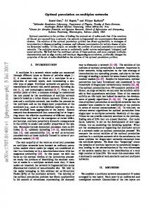
FIG. 1: Example of multiplex network with M = 2 layers. Nodes are the same in both layers. The connectivity at each layer is independent of each other, the connectivity inter-layer is from each node to itself (dashed links).

pled layered networks (multiplex network) where each layer could have very particular features different from the rest, and in this way, define a richer structure of interactions [3]. Multiplex networks are thus structured multilevel graphs in which interconnections between layers determine how a given node in a layer and its counterpart in another layer are linked and influence each other. Thus, they are essentially different from simple graphs with colored edges, multi graphs or hypergraphs and provide a mathematical ground for the analysis of many social networks (e.g. Facebook, Twitter, etc) and of several biological systems − for instance, in biochemical networks, many different signaling channels do actually work in parallel, giving raise to what is called multitasking, which can be modeled through a network of interconnected layers [4]. Although some works have recently focused on the description and analysis of interconnected networks [5–9], theoretically grounded results about general dynamical processes running on them are yet to come. In this Letter we focus on a particular setup of multilevel networks in which nodes are conserved through the different layers of the multiplex (see Fig. 1). The current study analyzes a diffusion process that takes place at the whole system level, i.e. within and across layers. This setup could account, for instance, for a diffusion dynamics taking place on top of a social network of contacts. Admittedly, the latter is a network of networks, i.e. the aggregate of many different social circles or subnetworks, each having its own temporal or structural patterns (for example, think of our online activity which includes different social networking sites such as Facebook, Twitter, etc.). The same applies to multimodal transportation networks [10], on top of which individuals “diffuse” within and between different layers (e.g. bus, subway, etc.). Let us remark, however, that our interest here is not to solve a specific real problem but to illustrate the analysis of diffusion processes on top of these structures. We propose a mathematical setting that allows to scrutinize the emergent diffusion time scales in multiplex networks. We concentrate on diffusive processes, as they constitute a good approximation for different types of dynamical processes (e.g.

2 synchronization and other nonlinear processes amenable of linearization [11]) whose dynamical properties can be captured by the behavior of the eigenvalues of the Laplacian matrix. For instance, the time needed to synchronize phase oscillators in a network is related to the second smallest eigenvalue of the Laplacian, λ2 [12], and the stability of the synchronized state is determined by the eigenratio λN /λ2 [13]. The spectral analysis of complex networks constitutes then still a promising area of research [14, 15]. Following a perturbative analysis of the spectra [16], our results allow to get new physical insight about diffusion processes through the analytical determination of the asymptotic behavior of the eigenvalues of the Laplacian of the multiplex (supra-Laplacian) when the diffusive coupling between layers is either small or large. Our findings prove that the emergent physical behavior of the diffusion process when considering coupled layered networks is far from trivial, in some cases (specified below) the coupling of networks shows a super-diffusive behavior meaning that diffusive processes in the multiplex are faster than in any of the networks that form it separately. Let us consider a set up in which the diffusive dynamics is linearly coupled within nodes in each layer K, through a diffusion constant DK , and among nodes in different layers K and L, in this case with a diffusion constant DKL . The network at each layer is assumed to be connected and undirected, but it can be weighted. The state of each of the N nodes is represented as a vector indexed by layers xK i (t) where the subscript stands for the node and the superscript for the layer. The equations describing the dynamical evolution of the states of the nodes, considering a multiplex of the M layers, are: M N X X dxK K K K i wij (xK − x )+ DKL (xL = DK j i i − xi ) , (1) dt j=1 L=1

K K where wij denotes the weight matrix at layer K (wij = 0 means that there is no link between nodes i and j in layer K). This set of equations can be dimensionally lifted to a space of N × M dimensions. To have a more clear picture of our formalism we will consider, without loss of generalization, the most simple case of two layers M = 2. First, we define a column vector state of 2N elements, (x11 · · · x1N |x21 . . . , x2N ) = (x1 |x2 ) = x. Then Eq. (1) can be written in matrix form, where the interaction matrix has a block structure that conforms an object we call supra-Laplacian L, with the same properties that any zero-sum rows Laplacian has: D1 L 1 + Dx I −Dx I L= , (2) −Dx I D2 L 2 + Dx I

where L1 and L2 are the respective Laplacians of each layer, and I is the identity matrix. Here we have replaced D12 by Dx to emphasize the role of the diffusion process among the same node at different layers. The Laplacian matrix of each layer K is just LK = SK − WK , where WK is the weights matrix at layer K, and SK a diagonal matrix containing P theKstrength of each node i at layer K, (SK )ii = sK i = j wij . Note

that the diagonal block structure of the supra-Laplacian reflects the interaction within layers and the off-diagonal blocks the connectivity between layers. The dynamical properties of the system can then be cast in terms of the eigenvalues of this matrix. Eq. (1) can be written as x˙ = −Lx and, given that L is symmetric, its solution in terms of normal modes is φi (t) = φi (0)e−λi t , where λi are the eigenvalues of L, see e.g. [17, 18]. The diffusion time scale τ of the multiplex is controlled by the smallest non-zero eigenvalue of L. Specifically, τ = 1/λ2 . To get a physical insight on these eigenvalues as a function of the different diffusion coefficients within layers (D1 and D2 ) and between layers (Dx ), we propose to analyze the whole system using perturbation theory. To simplify the notation, we choose the diffusion coefficients D1 = D2 = 1 fixing then the relative time scale of the problem. Let us consider the decomposition L = L0 + D, where L0 is the block diagonal matrix corresponding to the Laplacians of every layer, with zeros in the off-diagonal blocks, and D is formed by the rest of the elements. In matrix form it reads: ! ! I −I L1 0 + Dx . (3) L = L0 + D = 0 L2 −I I Let us start the discussion by considering Dx = 0. Then, the eigenvalues of L are the set formed by the union of the eigenvalues corresponding to the Laplacians of each layer L1 and L2 . The eigenvalues are 0 = λ11 < λ12 ≤ . . . λ1N and 0 = λ21 < λ22 ≤ . . . λ2N , respectively, while the eigenvalues of the supra-Laplacian matrix are 0 = λ1 = λ2 < λ3 ≤ . . . ≤ λ2n , being λ3 = min(λ12 , λ22 ). It is interesting to note that to analyze the eigenvector space it is convenient to move to a new basis where the space corresponding to λ1 = λ2 = 0 is spanned by vectors (1 · · · 1|1 · · · 1) and (1 · · · 1| − 1 · · · − 1) instead of the canonical (1 · · · 1|0 · · · 0) and (0 · · · 0|1 · · · 1). Now let us consider that the diffusion between layers is different from zero, Dx 6= 0. In this case, the supraLaplacian will have the trivial eigenvalue λ1 = 0 with corresponding eigenvector (1 · · · 1|1 · · · 1), and a non-trivial eigenvalue λ = 2Dx that corresponds exactly to the eigenvector (1 · · · 1| − 1 · · · − 1), since ! ! ! 1 0 1 = + 2Dx . (4) L −1 0 −1 Note that this eigenvalue always exists, but it will be the smallest non-zero one only when Dx is very small, as compared to D1 and D2 . Next, we focus our attention on the opposite limit, a very large diffusion coefficient [22] between layers Dx ≫ 1. Defining Dx = 1/ǫ, we can write !# ! " L1 0 I −I ˜ (5) = Dx L. +ǫ L = Dx −I I 0 L2 The spectrum of L˜ is considered here a perturbation of that at ǫ = 0. It is worth recalling that, for ǫ = 0, the spectrum

3 corresponds to that of the coupling matrix ! I −I , −I I

(6)

˜ 1 = 0 and λ ˜ 2 = 2) both which consists of two eigenvalues (λ N -degenerate and spanned by eigenvectors of the form (u|u) and (u|−u), i.e. vectors having identical or opposite values in the ith and (i + N )th components, respectively. Thus, in the limit Dx → ∞, the set of eigenvalues of L will split in two groups, one showing a linear divergent behavior λ ≈ 2Dx for the sub-space (u| − u), and another having a finite value λ as the result of the undetermined limit (0 · ∞) in Eq. (5) for the sub-space (u|u). Now, we use the common ansatz in perturbation theory and propose a perturbed solution in terms of both eigenvalues and eigenvectors: (0)

λi = λi vi =

(0) vi

(1)

+ O(ǫ2 ) ,

(1) ǫvi

+ O(ǫ2 ) ,

+ ǫλi +

(7)

where the super-indices within parentheses represent the order of the perturbation [19, 20]. Given that a set of eigenvalues of L will diverge linearly as 2Dx , we concentrate in proposing perturbations for the finite solutions. These correspond to consider the following perturbation of the eigenspectrum of ˜ L: ˜ = 0 + ǫλ ˜′ , λ ! u +ǫ v = u

u′1 u′2

!

.

(8)

˜ we ob˜ = λv Expanding to O(ǫ) the eigenvalue problem Lv tain: ! ! u (u′1 − u′2 ) + L1 u ′ ˜ ǫ = ǫλ + O(ǫ2 ) . (9) (u′2 − u′1 ) + L2 u u Matching each of the components in Eq. (9) we get: ˜′ u , L1 u + (u′1 − u′2 ) = λ ˜′ u , L2 u + (u′ − u′ ) = λ 2

1

(10)

that, after adding and subtracting Eqs. (10), transform into: ˜′ u (L1 + L2 )u = 2λ (L1 − L2 )u = 2(u′1 − u′2 )

(11)

From the system of Eqs. (11) it is revealed that u is an eigenvector of the network formed by the superposition of both layers’ laplacians, and that the eigenvalue of L, at first order in the expansion, is ˜′ = λs , λ=λ 2

(12)

being λs the eigenvalue of the superposition (L1 + L2 ) corresponding to the eigenvector u. Moreover, given that the vector

perturbation in Eq. (8) must be orthogonal (u|u) ⊥ (u′1 |u′2 ), we can also find the eigenvector of the superposition (L1 +L2 ) such that u′2 = −u′1 ≡ −u′ , then u′ =

1 (L2 − L1 )u. 4

(13)

Summarizing, the eigenvectors with finite (i.e. non divergent) eigenvalues of the supra-Laplacian L for a large value of the diffusion coefficient Dx = 1/ǫ between layers are λs u + ǫu′ ′ with eigenvalue , (14) v = u − ǫu′ 2 being u and λs the eigenvectors and corresponding eigenvalues of the superposition (L1 + L2 ). The physical insight obtained is the following, for low values of the diffusion coefficient between layers, the diffusion time scale of the global system is controlled by the inverse of 2Dx . This asymptotic result is valid until the order of Dx is similar to those of D1 and D2 . For large values of Dx the eigenspectrum splits into a set of values that diverges as 2Dx , and a set of finite values, associated to the superposition of the layers. The minimal eigenvalue different from zero turns out to be half the eigenvalue corresponding to the superposition of both layers λs /2. A comparison between the diffusion time scale of the independent layers and the whole multiplex is possible using known bounds about the eigenvalues of the Laplacians [21]. The time scale associated to the multiplex for Dx ≪ 1 is τ = 2D1 x that means that the cross-diffusion between layers is the limiting value of the diffusion spreading. On the other hand, the time scale associated to the multiplex for Dx ≫ 1 is τ ≈ 2/λs . This latter case is far less trivial than the previous one. Using the bounds in [21] we deduce the following result: λ1 + λ22 λs ≥ 2 ≥ min (λ12 , λ22 ) . 2 2

(15)

The above inequality implies that the diffusion in the multiplex will be faster than the diffusion in the slowest layer. Thus, as a consequence of the multiplex structure, at least one layer (the one with the largest diffusion time scale) has its diffusion speeded up. The emergence of a super-diffussion, i.e. the fact that the time scale of the multiplex is faster than that of both layers acting separately is, in general, not guaranteed and depends on the specific structures coupled together. Furthermore, the following inequality also holds [21]: 1 λs s + s2i 2N (16) ≤ min i + Dx , 2 2N − 1 i 2 being sK i the strength of node i at layer K. Finally, it is worth noticing that although the previous analysis assumes that the networks within layers are connected, we have also analyzed the case in which this hypothesis is relaxed. Imagine for example two layers such as one layer has two disconnected components. In this situation, the results hold in the limit Dx ≫ 1, and in the limit Dx ≪ 1 the

Eigenvalues of the supra-Laplacian

4 10

2

10

10

model allows switch on and off the consideration of isolated layers or the whole multiplex, simply by putting Dx = 0. For the example exposed, we observe a super-diffusion process for the whole multiplex, that means that the time scale associated to the whole multiplex network is smaller than that of layer 1 and layer 2 if they were considered independently, i.e. τ < τ1 < τ2 . Other examples comparing multiplex networks with 1000 nodes per layer, with different standard topologies, including clustered networks, are presented in the Supplemental Material accompanying this letter, all them showing perfect agreement with the developed analysis.

1

0

-1

10 -2 10

-1

0

1

2

lowest (different from zero) eigenvalue scales as αDx , with 0 < α ≤ 2 although the perturbed eigenvector is far more intricate.

In conclusion, we have developed a formalism to unveil the time scales of diffusive processes on multiplex networks. The approach has been specifically presented for a two-layer multiplex, in a particular set up in which nodes are preserved through layers. We obtained analytical results in the two asymptotic limits of small and large diffusion coefficients between layers. The findings show that the multiplex structure is able to speed up the less diffusive of the layers. In principle, it could also give rise to a super-diffusion process thus enhancing the diffusion of both layers. This striking result appears when one considers that the diffusion between the layers of the multiplex is faster than that occurring within each of the layers. Thus, it paves the way to the analysis of superdiffusion processes in real multiplex scenarios such as multimodal transportation systems. On more general grounds, given the wide applicability of the properties of the Laplacian to address many dynamical properties of networked systems, our results constitute a first step towards a better understanding of linear and nonlinear processes on top of multiplex structures. This work has been partially supported by the Spanish DGICYT Grants FIS2009-13364-C02-01, FIS2009-13730-C0202, FIS2008-01240, FIS2011-25167, MTM2009-13848, FET projects PLEXMATH (317614), MULTIPLEX (317532) and LASAGNE (318132), and the Generalitat de Catalunya 2009SGR-838. J.G.-G. is supported by the MICINN through the Ramón y Cajal Program. A.A. acknowledges the ICREA Academia Award.

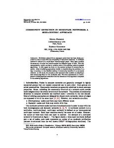
To illustrate our results, we have computed the evolution of the eigenvalues of the supra-Laplacian for the example represented in Fig. 1, which corresponds to two random networks of N = 6 nodes. In Fig. 2 (top) we plot the eigenvalues as a function of the diffusion coefficient Dx . We observe the splitting of the eigenvalues into two groups, divergent and finite values, as predicted. Fig. 2 (bottom) shows the theoretical estimates for λ2 in the asymptotic limits Dx ≪ 1 and Dx ≫ 1. Note that, except for the intermediate zone (Dx ≈ 1), where the analysis does not hold, the agreement is excellent. In this panel we have represented, as indicated in the legend, the eigenvalues of each layer, the eigenvalue of the superposition of both layers and the line corresponding to 2Dx as well as the eigenvalue of the supra-Laplacian. The results undoubtedly confirm that both theoretical limits (small and large Dx ) are correctly identified by the analytical derivations. Note that the

[1] M. Newman, Networks: An Introduction (Oxford University Press, Inc., New York, NY, USA, 2010). [2] P. J. Mucha, T. Richardson, K. Macon, M. A. Porter, and J.-P. Onnela, Science 328, 31 (2010). [3] K.-M. Lee, J. Y. Kim, W.-K. Cho, K.-I. Goh, and I.-M. Kim, New Journal of Physics 14, 033027 (2012). [4] E. Cozzo, A. Arenas, and Y. Moreno, Phys. Rev. E, in press (2012). [5] R. Parshani, S. V. Buldyrev, and S. Havlin, Physical Review Letters 105, 048701+ (2010). [6] S. V. Buldyrev, R. Parshani, G. Paul, H. E. Stanley, and S. Havlin, Nature (London) 464, 1025 (2010). [7] Y. Hu, B. Ksherim, R. Cohen, and S. Havlin, Phys. Rev. E 84, 066116 (2011).

10

10

10 Dx

10

10

2

1

λ2

10

λ2 of L1 λ2 of L2 λ2 of (L1+L2) / 2 λ = 2 Dx λ2 of Supra-Laplacian

10

0

-1

10 -2 10

10

-1

0

10 Dx

10

1

10

2

FIG. 2: (color online) Evolution of the eigenspectra of the toy model presented in Fig. 1 as a function of the coupling Dx (top) for D1 = D2 = 1, and comparison between the second smallest eigenvalues λ2 of the different Laplacians (bottom).

5 2

10

λ2 of L1 λ2 of L2 λ2 of (L1+L2) / 2 λ = 2 Dx

1

10

λ2

λ2 of Supra-Laplacian

0

10

-1

10

-2

10

-2

10

-1

10

0

10 Dx

1

10

2

10

Comparison between the second smallest eigenvalues λ2 of the different laplacians for a multiplex network consisting of two layers with 1000 nodes in each layer. The first layer contains a scale-free network with degree distribution P (k) ∼ k −2.5 , and the second layer contains a random Erdös-Rényi network with average degree hki = 8. 2

10


1

10

λ2

[8] J. Gao, S. V. Buldyrev, S. Havlin, and H. E. Stanley, Physical Review Letters 107, 195701 (2011). [9] J. Gao, S. V. Buldyrev, H. E. Stanley, and S. Havlin, Nature Physics 8, 40 (2012). [10] M. Barthélemy, Physics Reports 499, 1 (2011), ISSN 03701573. [11] A. Arenas, A. D´ıaz-Guilera, J. Kurths, Y. Moreno, and C. Zhou, Phys. Rep. 469, 93 (2008). [12] A. Almendral and A. D´ıaz-Guilera, New J. Phys. 9, 187 (2007). [13] M. Barahona and L. M. Pecora, Phys. Rev. Lett. 89, 054101 (2002). [14] S. Jalan, G. Zhu, and B. Li, Physical Review E 84, 046107+ (2011). [15] E. Estrada, N. Hatano, and M. Benzi, Physics Reports 514, 89 (2012). [16] P. V. Mieghem (Cambridge University Press, 2010). [17] A. Arenas, A. D´ıaz-Guilera, and C. J. Pérez-Vicente, Phys. Rev. Lett. 96, 114102 (2006). [18] A. Arenas, A. D´ıaz-Guilera, and C. J. Pérez-Vicente, Physica D 224, 27 (2006). [19] R. A. Marcus, The Journal of Physical Chemistry A 105, 2612 (2001). [20] S. Chauhan, M. Girvan, and E. Ott, Physical Review E 80, 056114+ (2009). [21] B. Mohar, in Graph Theory, Combinatorics, and Applications, edited by Y. Alavi, G. Chartrand, O. Oellermann, and A. Schwenk (Wiley, New York, NY, USA, 1991), pp. 871–898. [22] Strictly speaking if Dx = ∞ the model (1) does not hold and the whole multiplex can be understood as a single projected network with a unique state per node

0

10

-1

10

Supplemental material -2

10

2

10

1

10

λ2

0

10

-1

10

-2 -2

10

-1

10

-1

10

0

10 Dx

1

10

2

10

Comparison between the second smallest eigenvalues λ2 of the different laplacians for a multiplex network consisting of two layers with 1000 nodes in each layer. The first contains a scale-free network with degree distribution P (k) ∼ k −2.5 , and the second layer a small-world network with average degree hki = 8 and a replacement probability r = 0.3.

λ2 of Supra-Laplacian

10

-2

10 λ2 of L1 λ2 of L2 λ2 of (L1+L2) / 2 λ = 2 Dx

0

10 Dx

1

10

2

10

Comparison between the second smallest eigenvalues λ2 of the different laplacians for a multiplex network consisting of two layers with 1000 nodes in each layer. The first contains a scale-free network with degree distribution P (k) ∼ k −2.5 , and the second layer a scale-free network with degree distribution P (k) ∼ k −3 .

6 2

4

10

10 λ2 of L1 λ2 of L2 λ2 of (L1+L2) / 2 λ = 2 Dx

1

10


3

10

λ2 of Supra-Laplacian 2

λ2

λ2

10 0

10

1

10 -1

10

0

10

-2

10

-1

-2

10

-1

10

0

10 Dx

1

10

Comparison between the second smallest eigenvalues λ2 of the different laplacians for a multiplex network consisting of two layers with 1000 nodes in each layer. The first contains a scale-free network with degree distribution P (k) ∼ k −2.5 , and the second layer a 40 × 25 lattice with eight neighbors per node and periodic boundary conditions. 2

10


1

10

10

2

10

-1

10

0

10

1

10 Dx

2

10

3

10

Comparison between the second smallest eigenvalues λ2 of the different laplacians for a multiplex network consisting of two layers with 1000 nodes in each layer. The first contains a network structured in 4 communities of 250 nodes each, with average internal and external degrees hk int i = 105 and hk ext i = 105 respectively, and the second layer is similar but with hk int i = 200 and hk ext i = 10. The average clustering coefficients at each layer are 0.2336 and 0.7307 respectively, and the communities in both layers match. 4

λ2

10


0

10

3

10 -1

10

2

λ2

10

-2

10

-2

10

-1

10

0

10 Dx

1

10

2

10

Comparison between the second smallest eigenvalues λ2 of the different laplacians for a multiplex network consisting of two layers with 1000 nodes in each layer. The first contains a scale-free network with degree distribution P (k) ∼ k −2.5 , and the second layer has been obtained from a copy of the first layer network with 400 extra random links. Here we observe the absence of super-diffusion. This is a consequence of the semi-superposition (W1 + W2 )/2 being a (weighted) spanning graph of the network in the second layer W2 , thus according to Corollary 3.4 in [20] we have λ2 ((L1 + L2 )/2) ≤ λ2 (L2 ).

1

10

0

10

-1

10

-1

10

0

10

1

10 Dx

2

10

3

10

Comparison between the second smallest eigenvalues λ2 of the different laplacians for a multiplex network consisting of two layers with 1000 nodes in each layer. The first contains a network structured in 4 communities of 250 nodes each, with average internal and external degrees hk int i = 105 and hk ext i = 105 respectively, and the second layer is similar but with 17 communities, hk int i = 50 and hk ext i = 8. The average clustering coefficients at each layer are 0.2336 and 0.6541 respectively.