Optimal percolation on multiplex networks

Optimal percolation on multiplex networks Saeed Osat,1 Ali Faqeeh,2 and Filippo Radicchi2 1

Molecular Simulation Laboratory, Department of Physics, Faculty of Basic Sciences, Azarbaijan Shahid Madani University, Tabriz 53714-161, Iran 2 Center for Complex Networks and Systems Research, School of Informatics and Computing, Indiana University, Bloomington, Indiana 47408, USA

arXiv:1707.01401v1 [physics.soc-ph] 5 Jul 2017

Optimal percolation is the problem of finding the minimal set of nodes such that if the members of this set are removed from a network, the network is fragmented into non-extensive disconnected clusters. The solution of the optimal percolation problem has direct applicability in strategies of immunization in disease spreading processes, and influence maximization for certain classes of opinion dynamical models. In this paper, we consider the problem of optimal percolation on multiplex networks. The multiplex scenario serves to realistically model various technological, biological, and social networks. We find that the multilayer nature of these systems, and more precisely multiplex characteristics such as edge overlap and interlayer degree-degree correlation, profoundly changes the properties of the set of nodes identified as the solution of the optimal percolation problem.

I.

INTRODUCTION

A multiplex is a network where nodes are connected through different types or flavors of pairwise edges [1– 3]. A convenient way to think of a multiplex is as a collection of network layers, each representing a specific type of edges. Multiplex networks are genuine representations for several real-world systems, including social [4, 5], and technological systems [6, 7]. From a theoretical point of view, a common strategy to understand the role played by the co-existence of multiple network layers is based on a rather simple approach. Given a process and a multiplex network, one studies the process on the multiplex and on the single-layer projections of the multiplex (e.g., each of the individual layers, or the network obtained from aggregation of the layers). Recent research has demonstrated that accounting for or forgetting about the effective co-existence of different types of interactions may lead to the emergence of rather different features, and have potentially dramatic consequences in the ability to model and predict properties of the system. Examples include dynamical processes, such as diffusion [8, 9], epidemic spreading [10–13], synchronization [14], and controllability [15], as well as structural processes such as those typically framed in terms of percolation models [16–29]. The vast majority of the work on structural processes on multiplex networks have focused on ordinary percolation models where nodes (or edges) are considered either in a functional or in a non-functional state with homogenous probability [30]. In this paper, we shift the focus on the optimal version of the percolation process: we study the problem of identifying the smallest number of nodes in a multiplex network such that, if these nodes are removed, the network is fragmented into many disconnected clusters of non-extensive size. We refer to the nodes belonging to this minimal set as Structural Nodes (SNs) of the multiplex network. The solution of the optimal percolation problem has direct applicability in the context of robustness, representing the cheapest

way to dismantle a network [31–33]. The solution of the problem of optimal percolation is, however, important in other contexts, being equivalent to the best strategy of immunization to a spreading process, and also to the best strategy of seeding a network for some class of opinion dynamical models [34–37]. Despite its importance, optimal percolation has been introduced and considered in the framework of single-layer networks only recently [35, 36]. The optimal percolation is an NP-complete problem [32]. Hence, on large networks, we can only use heuristic methods to find approximate solutions. Most of the research activity on this topic has indeed focused on the development of greedy algorithms [31–33, 35]. The generalization of optimal percolation to multiplex networks that we consider here consists in the redefinition of the problem in terms of mutual connectedness [16]. To this end, we reframe several algorithms for optimal percolation from single-layer to multiplex networks. Basically all the algorithms we use provide coherent solutions to the problem, finding sets of SNs that are almost identical. Our main focus, however, is not on the development of new algorithms, but on answering the following question: What are the consequences of neglecting the multiplex nature of a network under an optimal percolation process? We compare the actual solution of the optimal percolation problem in a multiplex network with the solutions to the same problem for single-layer networks extracted from the multiplex system. We show that “forgetting” about the presence of multiple layers can be potentially dangerous, leading to the overestimation of the true robustness of the system mostly due to the identification of a very high number of false SNs. We reach this conclusion with a systematic analysis of both synthetic and real multiplex networks. II.

METHODS

We consider a multiplex network composed of N nodes arranged in two layers. Each layer is an undirected and unweighted network. Connections of the two layers are

encoded in the adjacency matrices A and B. The generic element Aij = Aji = 1 if nodes i and j are connected in the first layer, whereas Aij = Aji = 0, otherwise. The same definition applies to the second layer, and thus to the matrix B. The aggregated network obtained from the superposition of the two layers is characterized by the adjacency matrix C, with generic elements Cij = Aij + Bij − Aij Bij . The basic objects we look at are clusters of mutually connected nodes [16]: Two nodes in a multiplex network are mutually connected, and thus part of the same cluster of mutually connected nodes, only if they are connected by at least a path, composed of nodes within the same cluster, in every layer of the system. In particular, we focus our attention on the largest among these cluster, usually referred to as the Giant Mutually Connected Cluster (GMCC). Our goal is to find the minimal set of nodes that, if removed from the multiplex, leads to a GMCC that has at maximum √ a size equal to N . This is a common prescription, yet not the only one possible, to ensure that all clusters have non-extensive sizes in systems with a finite number of elements [35]. Whenever we consider single-layer networks, the above prescription apply to the single-layer clusters in the same exact way. We generalize most of the algorithms devised to find approximate solutions to the optimal percolation problem in single-layer networks to multiplex networks [31– 33, 35, 36]. Details on the implementation of the various methods are provided in the Supplementary Information (SI). We stress that the generalization of these methods is not trivial at all. For instance, most of the greedy methods use node degrees as crucial ingredients. In a multiplex network, however, a node has multiple degree values, one for every layer. In this respect, it is not clear what is the most effective way of combining these numbers to assign a single score to a node: they may be summed, thus obtaining a number approximately equal to the degree of the node in the aggregated network derived from the multiplex, but also multiplied, or combined in more complicated ways. We find that the results of the various algorithms are not particularly sensible to this choice, provided that a simple post-processing technique is applied to the set of SNs found by a given method. In Figure 1 for example, we show the performance of several greedy algorithms when applied to a multiplex network composed of two layers generated independently according to the Erd˝ os-Rényi (ER) model. Although the mere application of an algorithm may lead to different estimates of the size of the set of SNs, if we greedily remove from these sets the nodes that do not increase the size √ of the GMCC to the predefined sublinear threshold ( N ) [33], the sets obtained after this post-processing technique have almost identical sizes. As Figure 1 clearly shows, the best results, in the sense that the size of the set of SNs is minimal, is found with a Simulated Annealing (SA) optimization strategy [32] (see details in the SI). The fact that the SA method is outperforming score-based algorithms is not surprising. SA

Relative size of the largest cluster

2 1.0

0.5

0.0 0.0

High Degree High Degree Adaptive Collective Influence Explosive Immunization Simulated Annealing

0.1

0.2

Fraction of deleted nodes

0.3

Figure 1. Comparison among different algorithms to approximate solutions of the optimal percolation problem. We consider a multiplex network with N = 10, 000 nodes. The multiplex is composed of two network layers generated independently according to the Erd˝ os-Rényi model with average degree hki = 5. Each curve represents the relative size of the GMCC as a function of the number of nodes inserted in the set of SNs, thus removed from the multiplex. Colored markers indicate the effective fraction of nodes left in the set of SNs after a greedy post-processing technique is applied to the set found by the corresponding algorithm. The red cross identifies instead the size of the set of SNs found trough the Simulated Annealing optimization. Please note that the ordinate value of the markers has no meaning; in all √ cases, the relative size of the largest cluster is smaller than N . Details on the implementation of the various algorithms are provided in the SI.

actually represents one of the best strategies that one can apply in hard optimization tasks. In our case, it provides us with a reasonable upper-bound of the size of the set of SNs that can be identified in a multiplex network. The second advantage of SA in our context is that it doesn’t rely on ambiguous definitions of ingredients (as for example, the aforementioned issue of node degree). Despite its better performance, SA has a serious drawback in terms of computational speed. As a matter of fact, the algorithm can be applied only to multiplex networks of moderate size. As here we are interested in understanding the fundamental properties of the optimal percolation problem in multiplex networks, the analysis presented in the main text of the paper is entirely based on results obtained through SA optimization. This provides us with a solid ground to support our statements. Extensions, relying on score-based algorithms, of the same analyses to larger multiplex networks are qualitatively similar (see SI).

III. A.

RESULTS

The size of the set of structural nodes

We consider the relative size of the set of SNs, denoted by q, for a multiplex composed of two indepen-

A

0.6 0.75 0.4 0.50 0.2 0.25 0.0 0.00 0.0 2 4

Ordinary perc. (layer A) Ordinary perc. (aggregated)

101

Multiplex Layer A Layer B Aggregated

6 0.2 8 10 12 0.4 14

Relative error

Relative size of the structural set

1.00 0.8

100 10−1

B

0.6 2 4

Average degree

6

0.8 8 10 12 1.0 14

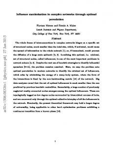
Figure 2. Optimal percolation problem in synthetic multiplex networks. A) We consider multiplex networks with N = 1, 000 and layers generated independently according to the Erd˝ osRényi model with average degree hki. We estimate the relative size of the set of SNs on the multiplex as a function of hki (green circles), and compare with the same quantity but estimated on the individual layers (black squares, red down triangles) or the aggregated (orange right triangles). B) Relative errors of single-layer estimates of the size of the structural set with respect to the ground-truth value provided by the multiplex estimate. Colors and symbols are the same as those used in panel A. The blue curves with no markers represent instead the results for an ordinary site percolation process [16].

dently fabricated ER network layers as a function of their average degree hki. We compare the results obtained applying the SA algorithm to the multiplex, namely qM , with those obtained using SA on the individual layers, i.e., qA and qB , or the aggregated network generated from the superposition of the two layers, i.e., qS . By definition we expect that qM ≤ qA ' qB ≤ qS . What we don’t know, however, is how bad/good are the measures qA , qB and qS in the prediction of the effective robustness of the multiplex qM . For ordinary random percolation on ER multiplex networks with negligible overlap, we know that qM ' 1 − 2.4554/hki [16], qA ' qB ' 1−1/hki, and qS ' 1−1/(2hki) [38]. Relative errors are therefore A ' B ' (2.4554−1)/(hki−2.4554), and S ' (2.4554 − 1/2)/(hki − 2.4554). We find that the relative error for the optimal percolation behaves more or less in the same way as that of the ordinary percolation (Figure 2B), noting that, as hki is increased, the decrease in the relative error associated with the individual layers is slightly faster than what expected for the ordinary percolation. The relative error associated with the aggregated network is instead larger than the one expected from the theory of ordinary percolation. As shown in Figure 2A, for sufficiently large hki, dismantling the ER multiplex network is almost as hard as dismantling any of its constituent layers.


3

0.4 0.3 0.2 0.0

Edge overlap and degree correlations

Next, we test the role played by edge overlap and layer-to-layer degree correlation in the optimal percolation problem. These are ingredients that dramatically

0.5

Relabeling probability

1.0

Figure 3. The effect of reducing edge overlaps and interlayer degree-degree correlation by partially relabeling nodes in multiplex networks with initially identical layers. Initially, both layers are a copy of a random network generated by an Erd˝ os-Rényi model with N = 1, 000 nodes and average degree hki = 5. Then, in one of the layers, each node is selected to switch its label with another randomly chosen node with a certain probability α. For each α, we determine the mean of the relative size of the set of SNs over 100 realizations of the SA algorithm on the multiplex network.

change the nature of the ordinary percolation transition in multiplex networks [26, 39–43]. In Figure 3, we report results of a simple analysis. We take advantage of the model introduced in Ref. [44], where a multiplex is constructed with two identical layers. Nodes in one of the two layers relabeled with a certain probability α. For α = 0, multiplex, aggregated network and single-layer graphs are all identical. For α = 1, the networks are analogous to those considered in the previous section. We note that this model doesn’t allow to disentangle the role played by edge overlap among layers and the one played by the correlation of node degrees. For α = 0, edge overlap amounts to 100%, and there is a one-to-one match between the degree of a node in one layer and the other. As α increases, both edge overlap and degree correlation decrease simultaneously. As it is apparent from the results of Figure 3, the system reaches the multiplex regime for very small values of α, in the sense that the relative size of the set of SNs deviates instantly from its value for α = 0. This is in line with what already found in the context of ordinary percolation processes in multiplex networks: as soon as there is a finite fraction of edges that are not shared by the two layers, the system behaves exactly as a multiplex [26, 39–43].

C. B.

Multiplex Single layer Aggregated

0.5

Accuracy and sensitivity

So far, we focused our attention only on the size of the set of SNs. We neglected, however, any analysis regarding the identity of the nodes that actually compose this set. To proceed with such an analysis, we note that different runs of the SA algorithm (or any algorithm with stochas-

4 tic features) generally produce slightly different sets of SNs (even if they all have almost identical sizes). The issue is not related to the optimization technique, rather to the existence of degenerate solutions to the problem. In this respect, we work with the quantities pi , each of which describes the probability that a node i appears in the set of SNs in a realization of the detection method (here, the SA algorithm). This treatment takes into account the fact that a node may belong to the set of SNs in a number of realizations of the detection method and may be absent from this set in some other realizations. Now, we define self-consistency of a detection P the P method as S = i p2i / i pi , which describes the ratio of the expected overlap between two SNs obtained from two independent realizations of the detection method to the expected size of an SN. If the set of SNs is identical across different runs, then S = 1. On the other hand, the minimal value we can observe is S = Q/N , assuming that the size of the structural set is equal to Q in all runs, but nodes belonging to this set are changing all the times, so that for every node we have pi = Q/N . As reported in Figure 4A, even for random multiplex networks, self-consistency is rather high for single layer representations of the network. On the other hand, S decreases significantly as the overlap and interlayer de-

A

0.8 Precision

Self consistency

1.0 0.8 0.6 0.8

0.6 0.2 0.4

0.0

0.5

0.4

0.8

C

0.7

0.2 0.6

Aggregated Layer A Layer B

0.6

0.2

1.0

F1 score

Recall

Multiplex Aggregated Layer A Layer B

0.4

B

0.0

0.5

1.0

0.5 0.8

1.0 1.0

D

0.6 0.4

0.5 0.0 0.0 0.0

0.2 0.5

0.4 1.0

0.0 0.6


Figure 4. The effect of reducing edge overlaps and interlayer degree-degree correlation by partially relabeling nodes in multiplex networks with initially identical layers. We consider the multiplex networks described in Figure 2 and the sets of SNs found for the multiplex and single layer based representations of these networks. A) As the set of SNs found in different instances of the optimization algorithm are different from each other, we first quantify the self-consistency of those solutions across 100 independent runs of the SA algorithm. We then assume that the multiplex representation provides the groundtruth classification of the nodes. We compare the results of the other representation with the ground truth by measuring their precision (panel B), their sensitivity or recall (panel C), and their F1 score (panel D).

gree correlations are decreased (Figure 4A). The low S values for multiplexes with small overlap and correlation together with the small sizes of their set of SNs (Figure 2) suggests that in such networks there can exist many relatively different sets of SNs that if nodes of each of these sets are removed the network is dismantled. Next, we turn our attention to quantifying how the sets of SNs identified in single-layer or aggregated networks are representative for the ground-truth sets found on the multiplex networks. Here, we denote by pi and wi the probability that node i is found within the set of SNs of, respectively, a multiplex network (ground truth) and a specific single-layer representation of that multiplex. To compare the sets represented by wi to the ground truth sets, we adopt three standard metrics in information retrieval [45, 46], namely precision, recall and the Van F1 score: Precision is defined as P Rijsbergen’s P P = [ i pi wi ]/[ i wi ], i.e., the ratio of the (expected) number of correctly detected SNs to the (expected) total number SNs. Recall is instead defined as P of detected P R = [ i pi wi ]/[ i pi ], i.e., the ratio of the (expected) number of correctly detected SNs to the (expected) number of actual SNs of the multiplex. We note that the selfconsistency we previously defined corresponds to precision and recall of the ground-truth set with respect to itself, thus providing a base line for the interpretation 2 of the results. The F1 score defined as F1 = 1/P +1/R provides a balanced measure in terms of P and R. As Figure 4B shows, precision deteriorates as the edge overlap and interlayer degree correlation decrease by increasing the relabeling probability. In particular, when the overlap and correlation between the layers of the multiplex network are not large, the precision of the sets of SNs identified in single layers or in the superposition of the layers is quite small (around 0.3), even smaller than the ratio of the qM of the multiplex to the q of any of these sets (see Figure 3). This means that, when the multiplex nature of the system is neglected, not only too many SNs are identified, but also a significant number of the SNs of the multiplex are not identified. Recall, on the other hand, behaves differently for single-layer and aggregated networks (Figure 4C). In single layers, we see that recall systematically decreases as the relabelling probability increases. The structural set of nodes obtained on the superposition of the layers instead provides large values of recall. This is not due to good performance rather to the fact that the set of SNs identified on the aggregated network is very large (see Figure 3). The results of Figure 4 demonstrate that even the larger recall values for the aggregated network do not lead to a better F1 score: the F1 score diminishes as the relabeling probability is increased.

D.

Real-world multiplex networks

In Table I, we present results of the analysis of optimal percolation problem on several real-world multiplex net-

5 Multiplex Network

Layers

N

[26] American Air. – Delta American Air. – United United – Delta [47, 48] Electric – Chem. Mon. C. Elegance Electric – Chem. Pol. Chem. Mon. – Chem. Pol. [49] physics.data-an – cond-mat.dis-nn Arxiv physics.data-an – cond-mat.stat-mech cond-mat.dis-nn – cond-mat.stat-mech [50, 51] Direct – Supp. Gen. Drosophila M. Direct – Add. Gen. Supp. Gen. – Add. Gen. [48, 50] Direct – Supp. Gen. Homo S. Physical – Supp. Gen.

84 73 82 238 252 259 1400 709 499 676 626 557 4465 5202

Air Transportation

Single layers

qM

S

qA

PA

RA F1(A)

0.12 0.10 0.10 0.09 0.12 0.25 0.05 0.03 0.02 0.01 0.01 0.09 0.05 0.05

0.85 0.99 1.00 0.69 0.79 0.82 0.78 0.73 0.50 0.62 0.81 0.82 0.72 0.75

0.14 0.16 0.27 0.16 0.15 0.28 0.10 0.08 0.06 0.07 0.07 0.14 0.16 0.15

0.58 0.32 0.23 0.41 0.50 0.69 0.38 0.23 0.13 0.12 0.06 0.44 0.20 0.23

0.70 0.52 0.62 0.71 0.63 0.77 0.77 0.67 0.46 0.60 0.64 0.74 0.73 0.77

0.63 0.40 0.34 0.52 0.56 0.73 0.51 0.34 0.20 0.20 0.11 0.55 0.31 0.35

Aggregate

qB

PB

RB F1(B)

0.32 0.14 0.12 0.26 0.39 0.39 0.07 0.03 0.04 0.11 0.09 0.12 0.13 0.13

0.29 0.68 0.80 0.22 0.24 0.51 0.55 0.64 0.23 0.09 0.05 0.50 0.23 0.22

0.79 1.00 1.00 0.60 0.78 0.79 0.75 0.72 0.51 0.64 0.59 0.70 0.64 0.63

0.42 0.81 0.89 0.32 0.37 0.62 0.63 0.68 0.32 0.16 0.09 0.58 0.34 0.33

qS

PS

RS F1(S)

0.35 0.25 0.33 0.35 0.45 0.42 0.13 0.09 0.09 0.19 0.16 0.20 0.27 0.26

0.32 0.39 0.30 0.21 0.22 0.48 0.31 0.22 0.13 0.07 0.04 0.35 0.15 0.16

0.92 1.00 1.00 0.79 0.82 0.80 0.81 0.74 0.65 0.87 0.87 0.80 0.89 0.90

0.47 0.56 0.46 0.33 0.35 0.60 0.45 0.34 0.22 0.13 0.08 0.49 0.26 0.27

Table I. Optimal percolation in real multiplex networks. From left to right we report the following information. The first three columns contain the name of the system, the identity of the layers, and the number of nodes of the network. The fourth and fifth columns are results obtained from the optimal percolation problem studied on the multiplex network, and contain information about the relative size qM , and self-consistency metric S of the set of SNs. Then, we report results obtained for the first single-layer network of the multiplex, namely the fraction qA of nodes in the structural set, the precision PA , the recall RA , and the F1 score of the set of SNs of the first layer. The next three columns are identical to those, but refer to the second layer. Finally, the three rightmost columns contain information about the fraction qS of nodes in the structural set, PS precision, RS recall, and the F1 score of the set of SNs for the aggregated network obtained from the superposition of the two layers. All results have been obtained with 100 independent instances of the SA optimization algorithm.

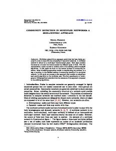
works generated from empirical data. For most of these networks, the optimal percolation on the multiplex rep-

Figure 5. Optimal percolation on the multiplex network of US domestic flights operated in January 2014 by American Airlines and Delta. The red circles represent the nodes that were a member of the set of structural nodes in different realizations of the optimal percolation on the multiplex representation of the network. The size of each circle is proportional to the probability of finding that node in the set of SNs. All other airports in the multiplex are represented as black squares. Interestingly, not all the 14 structural nodes match the top 14 busiest hubs [52], nor the probabilities follow the same order as the flight traffic of these airports. The results have been obtained with 100 independent instances of the SA optimization algorithm.

resentation has a rather high self-consistency. This implies that there is a certain small group of nodes that have a major importance in the robustness of such realworld networks to the optimal percolation process. The F1 score for most of the networks (not shown) is quite low indicating that on real-world networks we loose essential information about the optimal percolation problem if the multiplex structure is not taken into account. To provide a practical case study with a lucid interpretation, we depict, in Figure 5, the results for optimal percolation on a multiplex network describing the air transportation operated by two of the major airlines in the United States. SA identifies always 10 airports in the set of SNs. There is a slight variability among different instances of the SA optimization, with a total of 14 distinct airports appearing in the structural set at least once over 100 SA instances. However, changes in the SN set from run to run mostly regard airports in the same geographical region. Overall, airports in the structural set are scattered homogeneously across the country, suggesting that the GMCC of the network mostly relies on hubs serving specific geographical regions, rather than global hubs in the entire transportation system. For instance, the probabilities that describe the membership of the airports to the set of SNs do not strictly follow the same order as that of the recorded flight traffics [52]; nor merely the number of connections of the airports (not shown) is sufficient to determine the structural nodes. This is well consistent with the collective nature of the optimal percolation on the complex network of air transportation.

6 IV.

CONCLUSIONS

In this paper, we studied the optimal percolation problem on multiplex networks. The problem regards the detection of the minimal set of nodes (or set of structural nodes, SNs) such that if its members are removed from the network, the network is dismantled. The solution to the problem provides important information on the microscopic parts that should be maintained in a functional state to keep the overall system functioning, in a scenario of maximal stress. Our study focused mostly on the characterization of the SN sets of a given multiplex network in comparison with those found on the single-layer projections of the same multiplex, i.e., in a scenario where one “forgets” about the multiplex nature of the system. Our results demonstrate that, generally, multiplex networks have considerably smaller sets of SNs compared to the SN sets of their single-layer based network representations. The error committed when relying on single-layer representations of the multiplex doesn’t regard only the

[1] S. Boccaletti, G. Bianconi, R. Criado, C. I. Del Genio, J. G´ omez-Garde˜ nes, M. Romance, I. Sendi˜ na-Nadal, Z. Wang, and M. Zanin, Physics Reports 544, 1 (2014). [2] M. Kivel¨ a, A. Arenas, M. Barthelemy, J. P. Gleeson, Y. Moreno, and M. A. Porter, Journal of complex networks 2, 203 (2014). [3] K.-M. Lee, B. Min, and K.-I. Goh, The European Physical Journal B 88, 1 (2015). [4] M. Szell, R. Lambiotte, and S. Thurner, Proceedings of the National Academy of Sciences USA 107, 13636 (2010). [5] P. J. Mucha, T. Richardson, K. Macon, M. A. Porter, and J.-P. Onnela, science 328, 876 (2010). [6] M. Barthélemy, Physics Reports 499, 1 (2011). [7] A. Cardillo, J. G´ omez-Gardenes, M. Zanin, M. Romance, D. Papo, F. del Pozo, and S. Boccaletti, Scientific Reports 3, 1344 (2013). [8] S. G´ omez, A. D´ıaz-Guilera, J. G´ omez-Garde˜ nes, C. J. Pérez-Vicente, Y. Moreno, and A. Arenas, Phys. Rev. Lett. 110, 028701 (2013). [9] M. De Domenico, A. Solé-Ribalta, S. G´ omez, and A. Arenas, Proc. Natl. Acad. Sci. USA 111, 8351 (2014). [10] M. Dickison, S. Havlin, and H. E. Stanley, Phys. Rev. E 85, 066109 (2012). [11] A. Saumell-Mendiola, M. A. Serrano, and M. Bogu˜ na ´, Phys. Rev. E 86, 026106 (2012). [12] C. Granell, S. G´ omez, and A. Arenas, Phys. Rev. Lett. 111, 128701 (2013). [13] M. De Domenico, C. Granell, M. A. Porter, and A. Arenas, Nature Physics (2016). [14] C. I. del Genio, J. G´ omez-Garde˜ nes, I. Bonamassa, and S. Boccaletti, Science Adv. 2 (2016). [15] M. P´ osfai, J. Gao, S. P. Cornelius, A.-L. Barab´ asi, and R. M. D’Souza, Phys. Rev. E 94, 032316 (2016). [16] S. V. Buldyrev, R. Parshani, G. Paul, H. E. Stanley, and S. Havlin, Nature 464, 1025 (2010).

size of the SN sets, but also the identity of the SNs. Both issues emerge in the analysis of synthetic network models, where edge overlap and/or interlayer degree-degree correlations seem to fully explain the amount of discrepancy between the SN set of a multiplex and the SN sets of its single-layer based representations. The issues are apparent also in many of the real-world multiplex networks we analyzed. Overall, we conclude that neglecting the multiplex structure of a network system subjected to maximal structural stress may result in significant inaccuracies about its robustness.

ACKNOWLEDGMENTS

AF and FR acknowledge support from the US Army Research Office (W911NF-16-1-0104). FR acknowledges support from the National Science Foundation (Grant CMMI-1552487).

[17] R. Parshani, S. V. Buldyrev, and S. Havlin, Physical review letters 105, 048701 (2010). [18] R. Parshani, C. Rozenblat, D. Ietri, C. Ducruet, and S. Havlin, EPL (Europhysics Letters) 92, 68002 (2011). [19] G. Baxter, S. Dorogovtsev, A. Goltsev, and J. Mendes, Physical review letters 109, 248701 (2012). [20] S. Watanabe and Y. Kabashima, Phys. Rev. E 89, 012808 (2014). [21] S.-W. Son, G. Bizhani, C. Christensen, P. Grassberger, and M. Paczuski, EPL (Europhysics Letters) 97, 16006 (2012). [22] B. Min, S. Do Yi, K.-M. Lee, and K.-I. Goh, Physical Review E 89, 042811 (2014). [23] G. Bianconi, S. N. Dorogovtsev, and J. F. F. Mendes, Phys. Rev. E 91, 012804 (2015). [24] G. Bianconi and S. N. Dorogovtsev, Physical Review E 89, 062814 (2014). [25] F. Radicchi and A. Arenas, Nature Physics 9, 717 (2013). [26] F. Radicchi, Nature Phys. 11, 597 (2015). [27] D. Cellai and G. Bianconi, Physical Review E 93, 032302 (2016). [28] G. Bianconi and F. Radicchi, Phys. Rev. E 94, 060301 (2016). [29] F. Radicchi and G. Bianconi, Phys. Rev. X 7, 011013 (2017). [30] D. Stauffer and A. Aharony, Introduction to percolation theory (Taylor and Francis, 1991). [31] S. Mugisha and H.-J. Zhou, Phys. Rev. E 94, 012305 (2016). [32] A. Braunstein, L. DallAsta, G. Semerjian, and L. Zdeborov, Proceedings of the National Academy of Sciences 113, 12368 (2016). [33] L. Zdeborov´ a, P. Zhang, and H.-J. Zhou, Scientific Reports 6 (2016). [34] F. Altarelli, A. Braunstein, L. Dall’Asta, and R. Zecchina, Phys. Rev. E 87, 062115 (2013).

7 [35] P. Clusella, P. Grassberger, F. J. Pérez-Reche, and A. Politi, Phys. Rev. Lett. 117, 208301 (2016). [36] F. Morone and H. A. Makse, Nature 524, 65 (2015). [37] S. Pei, X. Teng, J. Shaman, F. Morone, and H. A. Makse, arXiv preprint arXiv:1606.02739 (2016). [38] M. Molloy and B. Reed, Random structures & algorithms 6, 161 (1995). [39] D. Cellai, E. L´ opez, J. Zhou, J. P. Gleeson, and G. Bianconi, Physical Review E 88, 052811 (2013). [40] G. Bianconi, Physical Review E 87, 062806 (2013). [41] B. Min, S. Lee, K.-M. Lee, and K.-I. Goh, Chaos, Solitons & Fractals 72, 49 (2015). [42] G. J. Baxter, G. Bianconi, R. A. da Costa, S. N. Dorogovtsev, and J. F. Mendes, Physical Review E 94, 012303 (2016). [43] D. Cellai, S. N. Dorogovtsev, and G. Bianconi, Physical Review E 94, 032301 (2016). [44] G. Bianconi and S. N. Dorogovtsev, arXiv preprint arXiv:1411.4160 (2014). [45] W. Chu and T. Y. Lin, Foundations and advances in data mining, Vol. 180 (Springer-Verlag, Berlin Heidelberg, 2005). [46] G. Maino and G. L. Foresti, Image Analysis and Processing – ICIAP 2011 , Vol. 6979 (Springer-Verlag, Berlin Heidelberg, 2011). [47] B. L. Chen, D. H. Hall, and D. B. Chklovskii, Proceedings of the National Academy of Sciences of the United States of America 103, 4723 (2006). [48] M. De Domenico, M. A. Porter, and A. Arenas, Journal of Complex Networks , cnu038 (2014). [49] M. De Domenico, A. Lancichinetti, A. Arenas, and M. Rosvall, Physical Review X 5, 011027 (2015). [50] C. Stark, B.-J. Breitkreutz, T. Reguly, L. Boucher, A. Breitkreutz, and M. Tyers, Nucleic acids research 34, D535 (2006). [51] M. De Domenico, V. Nicosia, A. Arenas, and V. Latora, Nature communications 6 (2015). [52] Wikipedia, List of the busiest airports in the United States.

1

Optimal percolation on multiplex networks Saeed Osat, Ali Faqeeh, Filippo Radicchi

Supplementary Information CONTENTS

S.1. Dismantling Algorithms A. High Degree (HD) B. High Degree Adaptive (HDA) C. Collective Influence (CI) D. Explosive Immunization (EI) E. Simulated Annealing (SA)

1 2 3 4 5 8

S.2. Greedy Reinserting (GR)

9

S.3. Complementary results for the degree-based methods References

10 12

S.1.

DISMANTLING ALGORITHMS

In this section, we briefly discuss some of the most effective dismantling algorithms on monoplex networks and their generalization to multiplex networks with two layers. The aim of these algorithms is to approximate the set of structural nodes which is the minimal set of nodes that their removal dismantles the network into vanishingly small (non-extensive) clusters. We first introduce some of the score-based algorithms. In such algorithms, at each step, a score for each node is calculated and the node with the highest score is removed (when several nodes have the same score, one of them is removed at random). We discuss four different types of such algorithms: High Degree (HD), High Degree Adaptive (HDA), Collective Influence (CI) and Explosive Immunization (EI). These methods are partially deterministic in nature, i.e., nearly the same set of structural nodes are discovered at each realizations of the algorithm. Besides score-based algorithms, we present Simulated Annealing (SA) algorithm which is a greedy algorithm that searches the solution space of the dismantling problem to find the best approximation to the structural sets. The SA method takes into account the collective behavior of the dismantling problem and provides several dismantling sets for different realizations of the algorithm on the same network structure.

2 A.

High Degree (HD)

In a monoplex network, the easiest way to dismantle a network, is a degree-based attack. After sorting the nodes with respect to their degrees, the nodes with the highest degree are removed one by one1 until the network is dismantled. As this algorithm is deterministic (except from the randomness in choosing a node from those with the same degree), the set of nodes that are removed to dismantle the network is almost unique. In multiplex networks, the degree of a node can be defined in various ways. We consider four different cases: the score of a node is defined as (i) its degree in layer A, (ii) its degree in layer B, (iii) the sum of its degrees across all the layers, and (iv) the product of its degrees across all the layers. It is worth mentioning that, when using HD, HDA and CI methods,


at each step we remove 0.001 × N of the nodes, where N is the total number of nodes (in

1.0

0.5 score(i) = kiA score(i) = kiB score(i) = kiA + kiB

0.0 0.0

score(i) = kiA ∗ kiB

0.1

0.2

0.3


Figure S-1. Optimal percolation for a multiplex network using the High Degree (HD) algorithm. We consider a multiplex network composed of two identical layers with N = 10000 nodes generated according to an Erd˝os–Rényi model with average degree hki = 5.0. Different line styles correspond to four different methods of defining node scores in multiplex networks. Markers are the dismantling fraction obtained with these four methods when combined with the Greedy Reinserting (GR) procedure (see Sec. S.2). 1

In cases where there are more than one node with a certain degree, one of them is removed at random.

3 each layer) of the multiplex. As Figure S-1 illustrates, to destruct a multiplex, the two scores defined as a combination of degrees in different layers are more effective than those based on the degrees in only one of the layers. In the main script and in the rest of the Supplemental Material (SM) when we refer to HD method, we mean the one in which a node degree is the product of its degrees across all the layers.

B.

High Degree Adaptive (HDA)

In the HD algorithm if we take into account the history of the process and recalculate, at each step, the degrees of the nodes, it is referred to as an HDA algorithm. Since the HDA algorithm is adaptive it is expected to work better than the HD method. In each step of the monoplex version of the HDA, we remove a fraction 0.001 × N of the nodes that had the highest degrees; then we recalculate the degree of the nodes present in the Giant Connected Component (GCC) of the network. We repeat this process until the size of the GCC reduces √ to N or smaller; this threshold satisfies the condition that in the dismantled network the


size of all the clusters is a sub-linear function of N .

Figure S-2.

1.0

0.5 score(i) = kiA score(i) = kiB score(i) = kiA + kiB

0.0 0.0

score(i) = kiA ∗ kiB

0.1

0.2


0.3

Performance of the HDA method on the same multiplex network considered in Fig-

ure S-1. Four different plots correspond to four different type of defining the degree of a node.

4 Like the HD case, we can define at least four methods to define the degree of a node. Please notice that in the multiplex version, when we update the degrees, we exclude those neighbors that are not in the Giant Mutually Connected Component (GMCC) of the network. Figure S-2 shows the effectiveness of the HDA algorithm for the different definitions of nodes’ degrees. Similar to the results for HD, it is more effective to combine the scores of different layers, than considering layers as isolated networks. In all the subsequent sections and in the main script, when we refer to HDA, we mean the one in which the score of a node is defined as the multiplication of its degrees across all the layers.

C.

Collective Influence (CI)

In the monoplex version of the CI algorithm [S1], the score CIi (l) of node i is equal to the excess degree of i multiplied by the sum of the excess degrees of its neighbours at a specific distance l from i: CIi (l) = (ki − 1)

X

j∈∂Ball(i,l)

(kj − 1),

(S.1)

where ∂Ball(i, l) denotes the neighbors of i at the distance l (i.e., the nodes that have a


geodesic distance l from i). At each step, the CI score is adaptively calculated for all the

1.0

0.5 CIi = CIA i CIi = CIB i B CIi = CIA i + CIi

0.0 0.0

B CIi = CIA i ∗ CIi

0.1

0.2


0.3

Figure S-3. The performance of the CI algorithm with l = 4 on the network of Figure S-1 using different definitions for the collective influence of a node.

5 nodes; then nodes with the highest score are removed from the network, until the network is dismantled. It was shown [S1, S2] that the performance of the CI method increases with l up to l = 4; for l > 4 the performance is not improved appreciably as l is increased. To adapt the CI algorithm to multiplex networks with two layers, we considered several possible definitions of the CI score in the multiplex: (i) using the CI obtained based only on the structure of layer A, (ii) based only on the structure of layer B, (iii) the sum of the CIs of a node in layer A and layer B, and (iv) the product of these two CI scores. Figure S-3 illustrates that, the generalizations of the CI method we considered here are not as effective as those derived based on the HD (Figure S-1) and HDA (Figure S-2) methods. Thus, methods based on the CI measures of the layers do not provide an effective algorithm for the optimal percolation problem.

D.

Explosive Immunization (EI)

The EI algorithm is based on a method referred to as explosive percolation. The original explosive percolation method was introduced by Achlioptas et al. [S3]. In this method at first all the edges are removed; then they are gradually reintroduced to the network, but in a specific order that prevents the formation of the GCC, until a point where the formation of the GCC is inevitable. To add a new edge, first several random edges are selected. Then a score is calculated for each of the selected edges using a predefined kernel2 . Then the edge with the minimum score is added back the network. The scores represent the contribution of each edge in the formation of the giant cluster. When the network reaches the point where the formation of the giant cluster is inevitable, the rest of the edges are added back using the same kernel. A problem related to explosive percolation is the optimal immunization [S4] in which the goal is to find the blocker nodes, which if get vaccinated, the giant connected component of the susceptible nodes breaks down; this break down eliminates a large scale epidemic spread. Clusella et al. [S4] proposed a reverse approach to find the blockers. They introduced an algorithm that locates instead all the nodes that are irrelevant to the formation of the giant susceptible cluster. In this respect, their algorithm is a modified version of the explosive per2

A possible kernel, for example, defines the score as the sum of the sizes of the two clusters connected by the corresponding edge.

6 colation. Their algorithm considers the site percolation version of the explosive percolation, in which all the links are present but, in the beginning, all the nodes are absent. Then, all the non-blocker nodes (that have no contribution to the formation of the giant susceptible cluster) are added gradually. The remaining nodes are the blocker nodes which should be vaccinated. We refer to this method as the explosive immunization (EI) algorithm. For a monoplex network we implement the EI algorithm as follows. At each step, we select N (C) = 1000 candidate nodes from the set of absent nodes, and calculate the score σi of each them using the following kernel: σi =

X q (eff) |Cj | − 1 + ki ,

(S.2)

j⊂Ni

where, Ni represents the set of all connected components (CCs) linked to node i, each of which has a size Cj , and ki

(eff)

is an effective degree attributed to each node (please see

Ref. [S4] for the details). Then the nodes with the lowest scores are added to the network. This procedure is continued until the size of the GCC exceeds a predefined threshold g ∗ √ (For the simulations of this paper we used g ∗ = N ). The minus one term in Eq. (S.2) is


excluding any leaves connected to node i, since they do not contribute to the formation of

1.0

0.5

0.0 0.0

Excluding leaves Including leaves

0.1

0.2

0.3


Figure S-4. Comparison between the performance of the EI method when we use Eq. (S.3) that p does not exclude the leaves and when we exclude the effect of leaves by replacing |M | in Eq. (S.3) p with |M | − 1. The results correspond to the same network as in Figure S-1.

7 the GCC and should be ignored in the score of a node. In our extension of the EI method to multiplex networks, we consider the different kernel but otherwise perform the exact same procedure as the one described above. The new kernel (Eq. (S.3)) we use is based on the sizes of the mutually connected components (MCCs) rather than on the sizes of CCs: q X q X q [A](eff) [B](eff) |Mj | + |Mj | + ki ki , σi = 1/2 [A]

where Ni

(S.3)

[B] j⊂Ni

[A] j⊂Ni

is the set of neighbors of node i in layer A, Mj is the size of the MCC to which [A](eff)

node j belongs, and ki

is the effective degree of i in layer A obtained using the same

definition proposed [S4] for the monoplex version of the EI method. In Eq. (S.3) we do not add a minus 1 term to exclude the leaves; the reason is that while in monoplex networks leaves do not have a significant contribution in the formation of the GCC, in multiplex networks even a leaf node is important in the formation of the GMCC. This is because at the sub-critical regime of multiplex networks usually most of the MCCs are isolated nodes or have very small sizes. Figure S-4 certifies that if the leaves were excluded instead, the performance of the algorithm would decrease. Figure S-5 shows that


the performance of the EI method does not depend appreciably on the number of candidate

1.0

0.5

0.0 0.0

N (C) N (C) N (C) N (C)

= 500 = 1000 = 5000 = 10000

0.1

0.2

0.3


Figure S-5. The results of the EI method do not depend appreciably on the number of candidate nodes N (C) . The simulations are performed on the same network used in Figure S-1.

8 nodes (N (C) ). In the simulations of Figure 1 of the main text, we used a N (C) = 1000.

E.

Simulated Annealing (SA)

The simulated annealing (SA) method has been used for the dismantling problem in monoplex networks [S5]. Generally an SA algorithm defines an energy function that attributes energy values to each configuration of the system. The phase space of the system is searched for the optimal configuration (the one with the minimum energy) by Markov Chain Monte Carlo moves that switch the system from one configuration to another. In dismantling of multiplex networks, the algorithm should find the minimal set of nodes which if deleted the size of the GMCC becomes non-extensive. Each configuration of the multiplex network is represented by {R, g}, where R and g are, respectively, the number of removed nodes (each node and all its corresponding replica nodes are counted as one node), and the relative size of the GMCC. The energy of a configuration is defined as follows: ε = Rv + g,

(S.4)

where v is the cost of removing a node from the multiplex network and in the simulations presented in this paper it is set v = 0.6. At each step t of the algorithm, one node, present or removed, is selected at random; then one of the following sets of operations are performed: • If the node is present and it belongs to the GMCC, it is removed (thus Rt = Rt−1 + 1) and the new size of the GMCC (gt ) is calculated. • If the node is present but it does not belong to the GMCC, then it is removed (thus Rt = Rt−1 + 1); but since it did not belong to the GMCC, gt = gt−1 . • If the node is in the set of removed nodes, it is added back to the network and Rt = Rt−1 − 1. Then Mi (the size of the MCC formed after inserting i) is calculated and gt = max (Mi , gt−1 ). Afterwards the energy of the new configuration εt is calculated and the set of operations is accepted with a probability equal to min 1, e−β(εnew −ε) . If it is accepted, the new configuration ({Rt , gt }) is retained, otherwise, the operations are omitted and the old configuration

({Rt−1 , gt−1 }) is preserved. Here, β is interpreted as the inverse of the temperature of the annealing process. The SA algorithm starts with a βmin and, at each step, β is slightly increased by δβ. A smaller δβ

9 means a slower decrease in the temperature which allows the SA method to better search for the optimal configurations, at the expense of increasing the running time of the algorithm. In this paper we change the values of β from 0.5 to 20.0 with δβ = 10−6 . In Figure 1 of the main text, we show that the SA method outperforms the four scorebased algorithms; thus, for the analysis of the optimal percolation problem, we mostly use the SA method (see the main text). In Sec. S.3, we also provide results for the second best algorithm, i.e., the HDA method and show that the results are qualitatively similar to those of the SA method.

S.2.

GREEDY REINSERTING (GR)

After a network (either isolated or multiplex) is dismantled using a greedy or score-based algorithm, there are some removed nodes that if added back to the network, the size of the GMCC is not increased substantially, i.e., no cluster with an extensive size is created if they are reinserted. Such nodes may have been removed because the greedy or scorebased algorithms are not exact in the sense that they do not take into account the collective nature of the dismantling problem. An approach that addresses this issue is referred to as the greedy reinserting (GR) method [S2, S5]. In the GR method, after a set of structural nodes is detected using another algorithm, at each step a randomly chosen node from the set is reinserted to the network, and unless its reinsertion does not increase the size of the √ GMCC to a threshold N , it is removed again. This process is continued until practically none of the nodes remained in the set can be added to the network without keeping the size of the GMCC non-extensive. As shown in Figures S-1–S-5 and Figure 1 of the main text, the GR method boosts effectively the performance of every one of the score-based dismantling algorithms and returns sets of structural nodes with almost identical sizes irrespective of the initial algorithm used. Moreover, the result of each of the score-based algorithms combined with the GR method is nearly as good as that of the SA method (the SA method itself is not improved appreciably by applying a GR method afterwards). These results suggest that probably the sets obtained by the SA method and any one of the score-based algorithms combined with GR are to a considerable extent similar to each other. In Sec. S.3 we show that actually the results of HDA and those of SA are qualitatively similar.

10 S.3.

COMPLEMENTARY RESULTS FOR THE DEGREE-BASED METHODS

In this section, we provide further results for the HD (Figure S-6) and the HDA (Figure S7) methods, and also for the combination of the GR method with HDA (Figures S-8–S-9); we compare these results with some of the results of the SA algorithm presented in the main text. In contrast to the SA algorithm, the degree-based algorithms are much more efficient in terms of the running time; hence, we were able to produce some of the results (see Figures S-6–S-7) for larger ER networks. Figures S-6 and S-7 show that, for both HD and HDA performed on the aggregated

1.0 0.8

A


101

0.6 0.4 0.2 0.0 0.0 2 4


Relative error


representation, the behavior of qc (the relative size of the set of structural nodes) with

100 10−1

6 0.2 8 10 12 0.4 14

B

0.6 2 4

Average degree

6

0.8 8 10 12 1.0 14

Figure S-6. Like Figure 2 of the main script. Dismantling of a multiplex network with each layer generated independently according to the Erd¨ os-Rényi model with average degree hki and N = 105

1.0 0.8 0.8 0.6 0.6 0.4 0.4 0.2 0.2

A


101

0.0 0.0 2 4


6 0.2 8 10 12 0.4 14

Relative error


using the HD method.

100 10−1

B

0.6 2 4

Average degree

6

0.8 8 10 12 1.0 14

Figure S-7. Like Figure S-6, for the HDA algorithm.


11

Multiplex Single layer Aggregated

0.5 0.4 0.3 0.2 0.0

0.5


1.0

Figure S-8. Optimal percolation results the using HDA+GR method on the networks of Figure 3 of the main script.

respect to the network average degree resembles the results of the SA algorithm. On the other hand, HDA+GR matches better to the result of SA for optimal percolation on each of the single layers of the multiplex network. In particular, for networks with sufficiently large degree, HDA on each of the layers can find a qc very close to the qc it obtains for the multiplex representation. As shown in Figure S-8, the behavior of qc with respect to the relabeling probability3 obtained with the HDA+GR method is qualitatively similar to the results of the SA algorithm (Figure 3 of the main text). Moreover, Figure S-9A shows that, as expected, HDA+GR has a relatively higher self-consistency compared to that of the SA algorithm reported in Figure 4 of the main text. It is worth noting that, in contrast to SA, the self-consistency of HDA+GR does not decrease with the relabeling probability in the multiplex representation (Figure S-9A). Interestingly, despite the qualitative similarity of the results, HDA+GR returns higher values of precision (Figure S-9B), recall (Figure S-9C), and F1 -score (Figure S-9D) than those of SA (see Figure 4 of the main text). As there is not much randomness in HDA+GR, the structural nodes are dominantly determined by the sequence of (adaptive) degrees of the nodes and the sets from different network representations have a higher overlap compared 3

higher relabeling probability indicates lower density of overlapping edges and lower interlayer degree-degree correlation.

12

A

0.6

1.0 0.4

Precision

0.8 0.8

0.6 0.4 0.0

Recall

0.8


0.5

B

Layer A Layer B Aggregated

0.6 0.4

1.0

0.0

C

0.8 F1 score

Self consistency

1.0

0.8 0.2

0.5

1.0

0.5 0.8

1.0

D

0.6

0.6 0.0 0.0

0.2 0.5

0.4 1.0

0.4 0.0 0.6


Figure S-9. Results for the performance of the HDA+GR method using the same measures employed in Figure 4 of the main script.

to those find by the SA algorithm.

[S1] F. Morone and H. A. Makse, Nature 524, 65 (2015). [S2] L. Zdeborová, P. Zhang, and H.-J. Zhou, Scientific Reports 6 (2016). [S3] D. Achlioptas, R. M. D’souza, and J. Spencer, Science 323, 1453 (2009). [S4] P. Clusella, P. Grassberger, F. J. Pérez-Reche, and A. Politi, Phys. Rev. Lett. 117, 208301 (2016). [S5] A. Braunstein, L. DallAsta, G. Semerjian, and L. Zdeborov, Proceedings of the National Academy of Sciences 113, 12368 (2016).